As usual, the first thing we do is to get your data into the app. So far, you only have the US data; however, in anticipation of the farmers' markets point data, we will haul in a little later—let's use d3.queue() to load our data:

d3.queue()
  .defer(d3.json, 'data/us.json')
  .await(ready);

The ready() function gets called asynchronously as soon as the data is loaded:

function ready(error, us) {
  if (error) throw error;

  var us = prepData(us);
  drawGeo(us);

}

In there, you check for errors, prepare the US data, and draw it. The data preparation is a one-liner, converting the topo to an array of GeoJSON polygons:

function prepData(topo) {
  var geo = topojson.feature(topo, topo.objects.us);
  return geo;
}

The drawing function takes the GeoJSON as its only argument. Create the projection and the path generator and draw the US. projection is a global variable as we will use it in other places later:

function drawGeo(data) {
  projection = d3.geoAlbers() // note: global
    .scale(1000).translate([width/2, height/2]);

  var geoPath = d3.geoPath()
    .projection(projection);

  svg
    .append('path').datum(data)
      .attr('d', geoPath)
      .attr('fill', '#ccc')
}

Note that we are using the d3.geoAlbers() projection here. The Albers projection is a so-called equal area-conic projection, which distorts scale and shape but preserves area. This is essential when producing dot density or hexbin maps to not distort the perceived density of the dots across distorted areas. To put it differently, our hexbins represent equal areas on the projected plane, hence we need to make sure that the projected plane honors equal areas with an appropriate projection. Note that equal area-conic projections require the map maker to pick two parallels (circles of latitude) on which the projection is based. d3.geoAlbers has been already preconfigured, picking the two parallels [29.5, 45.5]. This produces an optimized projection for the US. When visualizing other countries or map areas, you can overwrite this with the .parallels() method or set it up yourself with the d3.geoConicEqualArea() projection.

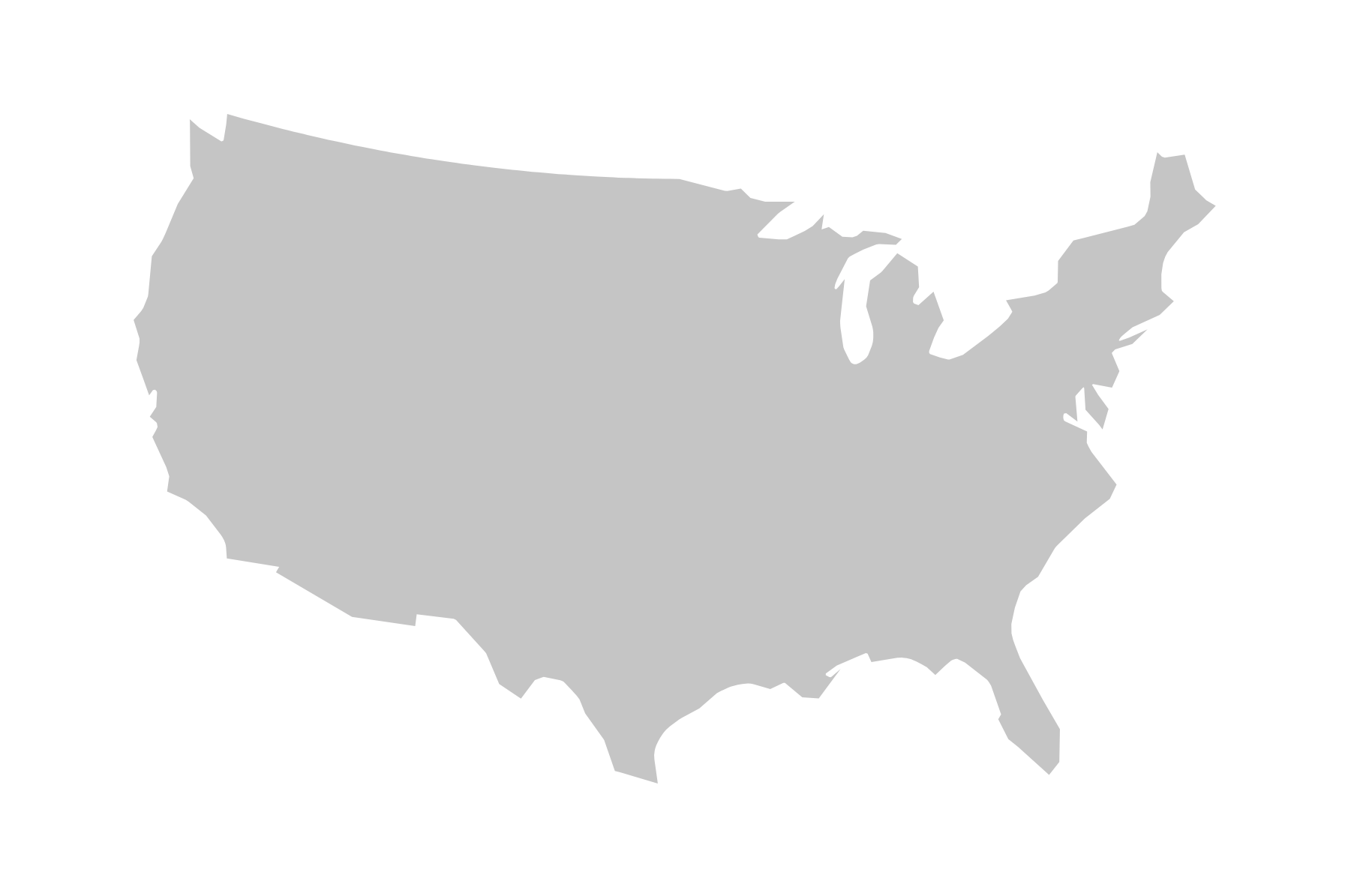
The result is not too surprising:

Before we move on, let's take one step back and look at how we produced the TopoJSON data on the command line. The original US map data comes in a shapefile from https://www.census.gov/geo/maps-data/data/cbf/cbf_nation.html and is converted from shapefile to TopoJSON in six steps as follows:

1. Install shapefile, if you haven’t yet:

npm install -g shapefile 

2. Install topojson, if you haven’t yet:

npm install -g topojson

3. Convert the shapefile to GeoJSON:

shp2json cb_2016_us_nation_20m.shp --out us-geo.json 

4. Convert the Geo to TopoJSON:

geo2topo us-geo.json > us-topo.json 

5. Compress number precision:

topoquantize 1e5 < us-topo.json > us-quant.json 

6. Simplify the geometry:

toposimplify -s 1e-5 -f < us-quant.json > us.json