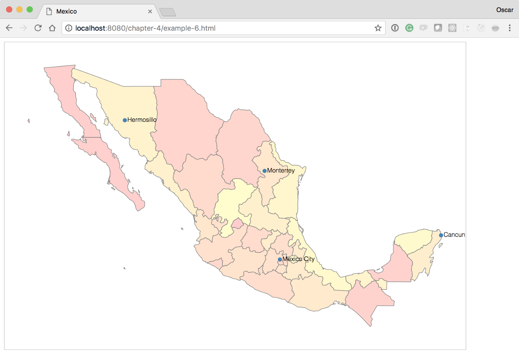
So far, everything we have done has involved working directly with the geographic data and map. However, there are many cases where you will need to layer additional data on top of the map. We will begin slowly by first adding a few cities of interest to the map of Mexico.

This experiment will, again, require us to start with example-3.html. The complete experiment can be viewed at: http://localhost:8080/chapter-4/example-6.html.

In this experiment, we will add a text element to the page to identify the city. To make the text more visually appealing, we will first add some simple styling in the <style> section:

text{ 
  font-family: Helvetica; 
  font-weight: 300; 
  font-size: 12px; 
} 

Next, we need some data that will indicate the city name, the latitude, and longitude coordinates. For the sake of simplicity, we have added a file with a few starter cities. The file called cities.csv is in the same directory as the examples:

name,lat,lon, 
Cancun,21.1606,-86.8475 
Mexico City,19.4333,-99.1333 
Monterrey,25.6667,-100.3000 
Hermosillo,29.0989,-110.9542 

Now, add a few lines of code to bring in the data and plot the city locations and names on your map. Add the following block of code right below the exit section (if you are starting with example-2.html):

    d3.csv('cities.csv', function(cities) { 
      var cityPoints = svg.selectAll('circle').data(cities); 
      var cityText = svg.selectAll('text').data(cities); 
 
      cityPoints.enter() 
          .append('circle') 
          .attr('cx', function(d) {
             return projection ([d.lon, d.lat])[0]
          })
          .attr('cy', function(d) {
             return projection ([d.lon, d.lat])[1]
          }) 
          .attr('r', 4) 
          .attr('fill', 'steelblue'); 
 
      cityText.enter() 
          .append('text') 
          .attr('x', function(d) {
             return projection([d.lon, d.lat])[0]})
          .attr('y', function(d) {
             return projection([d.lon, d.lat])[1]}) 
          .attr('dx', 5) 
          .attr('dy', 3) 
          .text(function(d) {return d.name}); 
    }); 

Let's review what we just added.

The d3.csv function will make an AJAX call to our data file and automatically format the entire file into an array of JSON objects. Each property of the object will take on the corresponding name of the column in the .csv file. For example, take a look at the following lines of code:

[{ 
  "name": "Cancun",  
  "lat":"21.1606",  
  "lon":"-86.8475" 
}, ...] 

Next, we define two variables to hold our data join to the circle and text the SVG elements.

Finally, we will execute a typical enter pattern to place the points as circles and the names as text SVG tags on the map. The x and y coordinates are determined by calling our previous projection() function with the corresponding latitude and longitude coordinates from the data file.

Note that the projection() function returns an array of x and y coordinates (x, y). The x coordinate is determined by taking the 0 index of the returned array. The y coordinate is determined from the index, 1. For example, take a look at the following code:

.attr('cx', function(d) {return projection([d.lon, d.lat])[0]})  

Here, [0] indicates the x coordinate.

Your new map should look like the one shown in the following screenshot: