So far, we only had eyes for the base layer setup, visualising our layout points as hexagons. Now, we’ll finally add some real data to it. First, we need to load it to our d3.queue():

d3.queue()
  .defer(d3.json, 'data/us.json')
  .defer(d3.json, 'data/markets_overall.json')
  .await(ready);

In the ready() function, we just add another line to our visualization pipeline, triggering a function that will prepare the data for us:

function ready(error, us) {
  // … previous steps
  var dataPoints = getDatapoints(markets)
}

getDatapoints() simply takes in the loaded CSV data and returns a more concise object boasting x and y screen coordinates as well as the datapoint flag, indicating that this is not a layout point but an actual data point. The rest is market-specific data, such as name, state, city, and url, we can use to add as info to each hexagon:

function getDatapoints(data) {

  return data.map(function(el) {
    var coords = projection([+el.lng, +el.lat]);
    return {
      x: coords[0],
      y: coords[1],
      datapoint: 1,
      name: el.MarketName,
      state: el.State,
      city: el.city,
      url: el.Website
    }
  });

}

Back in the ready() function, you just concatenate these data points to the layout points for the complete dataset you will use for your final hexbin map:

function ready(error, us) {
  // … previous steps

  var dataPoints = getDatapoints(markets)
  var mergedPoints = usPoints.concat(dataPoints)
}

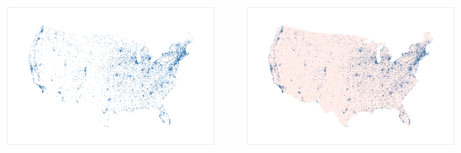
Here’s the markets data visualized as a classic dot density map in blue as well as together with the grid layout data in red: