Our aim is to draw a hexagon grid across the US map. D3-hexbin will do this for us later, but it can only draw a hexagon where there are points. So, we need to feed points to it. These points won’t have any information value for our users. They will only be used to produce the layout. As such, we can distinguish two types of points we will need:

• Layout points to produce the hexbin tiling
• Datapoints to render the color-scaled information

We’ll get to the datapoints soon, but at this stage, we’re only concerned with our layout points. Once done, you will have produced this wonderfully regular pattern of points stretching across our entire drawing area:

In the next step, we will cut this grid to shape to fit the US silhouette, but let’s lay it out first. Note that this will be the most involved bit of the calculations. No rocket science, but don’t worry if it doesn’t click immediately. Things often become clearer once stepping through the code in the debugger and/or using a few console.log()’s. Anyway, here we go:

var points = getPointGrid(160);

getPointGrid() takes only one argument: the number of columns of points we want. That’s enough for us to calculate the grid. First, we will get the distance in pixels between each dot. The distance between each dot stands in for the distance between the hexagon centers. d3.hexbin() will calculate this for us precisely later, but, for now, we want to get a good approximation. So, if we decide to have 160 columns of dots and our width is 840, the maximum distance will be 840 / 160 = 5.25 pixels. We then calculate the number of rows. The height is 540, so we can fit in 540 / 5.25 rows, which equals 108 rows of dots if we round it down:

function getPointGrid(cols) {
  var hexDistance = width / cols;
  var rows = Math.floor(height / hexDistance);

  hexRadius = hexDistance/1.5;

Next, we will calculate the hexRadius. This might look funny. Why divide the distance by 1.5? The D3-hexbin module will produce hexbins for us if we feed it points and a desired hexbin radius. The hexagon radius we set here should guarantee that the resulting hexagons are large enough to include at least one point of the grid we produce. We want a gap-free hexagon tiling after all. So, a tight grid should have a small radius, and a wide grid should have a wider radius. If we had a wide grid and a small radius, we wouldn’t get a hexagon for each point. There would be gaps.

Luckily, hexagons are regular shapes, and their dimensions and properties are nicely interconnected. The vertical distance between hexagon centers is 1.5 times its radius, the horizontal distance is √3 (roughly 1.73):

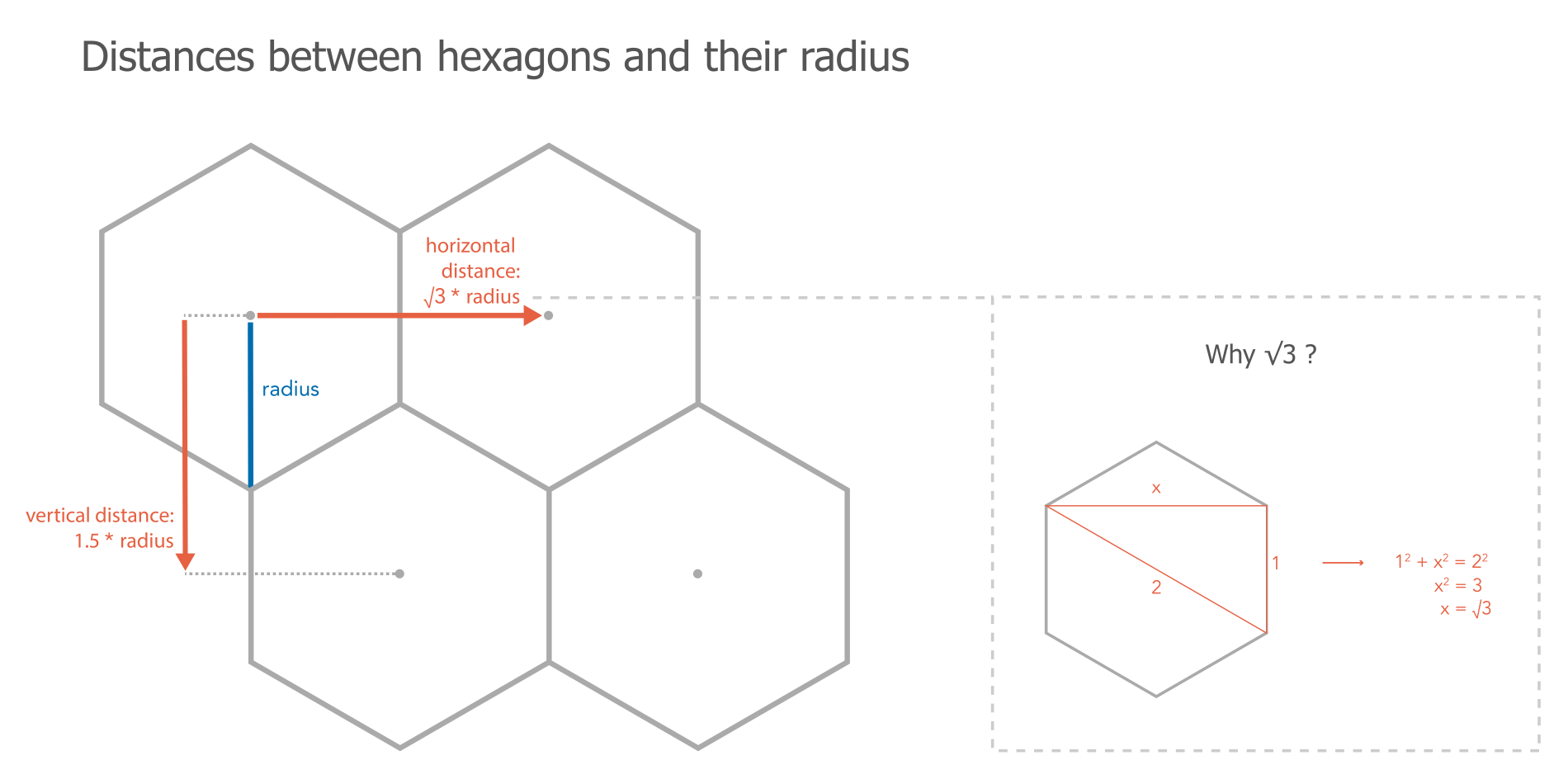
Our grid points work as a proxy of hexagon centers. As such they are not 'perfectly' laid out in the sense that their vertical distance is the exact same as their horizontal distance with 5.25 pixels. In a perfect hexagon grid the vertical distance would be a little shorter than the horizontal distance as you can see in above figure. In order to get a relatively tight mesh of hexagons on the base of our proxy grid, we should chose a safe—meaning wide—radius to pass to the D3-hexbin module which indeed will deliver a perfect hexagon grid. We can calculate this radius with the formulae in the preceding figure as well as our distance (5.25 pixel) by solving for Radius. When re-shuffling the equation for the vertical distance Distance = 1.5 * Radius becomes Radius = Distance / 1.5. In our case the distance is 5.25 / 1.5 = a radius of 3.5. Using the horizontal distance would have given us a less safe—meaning tighter—radius with 5.25 / √3 = 3.03, which in fact would produce a few gaps in our final tiling.

Next, we will create and return the grid immediately—well, the coordinates for the grid that is:

return d3.range(rows * cols).map(function(el, i) {
    return {
      x: Math.floor(i % cols * hexDistance),
      y: Math.floor(i / cols) * hexDistance,
      datapoint: 0
    }
  });
} // end of getPointGrid() function

d3.range(rows * columns) creates an array with one element per dot. We then iterate through each dot with .map() returning an object with three properties: x, y, and datapoint. These properties will define each of our grid points. The x coordinate will increase by the hexDistance every point and reset to 0 for each row (or put differently, after it runs through all columns). The y coordinate will increase by the hexDistance for each new row.

Equally important, each of these grid points will get a property called datapoints, which we will set to 0. This property will distinguish all the layout points (0) from the data points (1) later, allowing us to focus on the latter.

Congratulations! This was the most difficult bit, and you’re still here proudly lifting a square grid of tomato-colored dots into the air.

function drawPointGrid(data) {
  svg.append('g').attr('id', 'circles')
    .selectAll('.dot').data(data)
    .enter().append('circle')
      .attr('cx', function(d) { return d.x; })
      .attr('cy', function(d) { return d.y; })
      .attr('r', 1)
      .attr('fill', 'tomato');
}