For a moment, let's pretend that TopoJSON does not exist and illustrate how only GeoJSON can be used to create a map. This will help illustrate the need for TopoJSON in the next section. The following code snippet is a quick example to tie everything together; you can also open example-1.html from the chapter-6 folder (http://localhost:8080/chapter-6/example-1.html) to see the map in your browser of the following code:

  d3.json('geojson/spain-geo.json', function(data) { 
    var b, s, t; 
    projection.scale(1).translate([0, 0]); 
    var b = path.bounds(data); 
    var s = .9 / Math.max((b[1][0] - b[0][0]) / width, 
     (b[1][1] - b[0][1]) / height);    
     var t = [(width - s * (b[1][0] +
     b[0][0])) / 2, 
     (height - s * (b[1][1] + b[0][1])) / 2]; 
    projection.scale(s).translate(t); 
 
    map = svg.append('g').attr('class', 'boundary'); 
    spain = map.selectAll('path').data(data.features); 

Notice that the code is almost identical to the examples in the previous chapters. The only exception is that we are not calling the topojson function (we will cover why topojson is important next). Instead, we are passing the data from the AJAX call directly into the data join for the following enter() call:

    spain.enter() 
       .append('path') 
       .attr('d', path); 
 
 }); 

As predicted, we have our map of Spain:

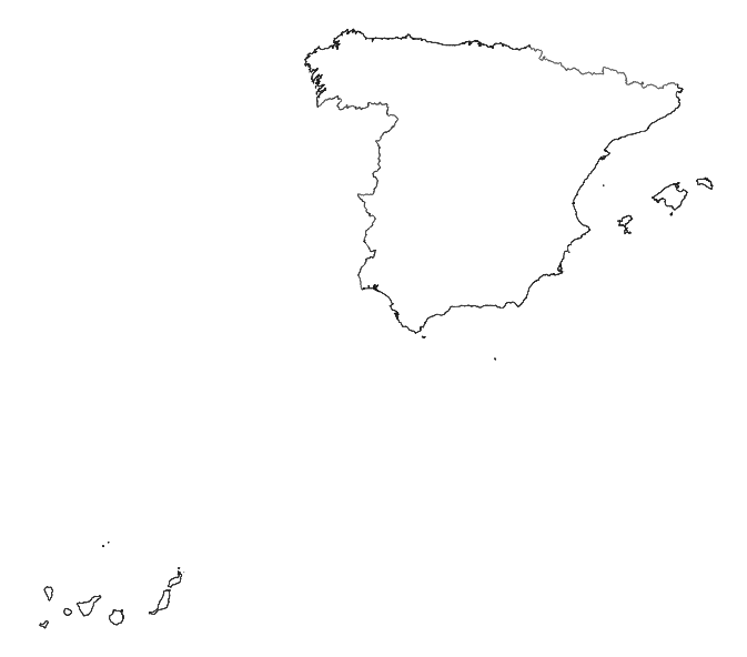
While using GeoJSON directly may seem like the best approach, there are some problems. Primarily, a one-to-one conversion of an Esri shapefile to the GeoJSON format contains a lot of detail that is probably unnecessary and will create a huge GeoJSON file. The larger the file, the more time it will take to download. For example, spain-geo.json produced an almost 7 MB GeoJSON file.

Next, we will explore how TopoJSON can help by modifying several optimization levers while still maintaining significant details.