Hexagons can solve some of the problems we mentioned in the preceding section. They can help the unequal area problems of choropleth maps and can bring ordered focus to point clusters. Let’s look at a few first:

As you can see, hexagons have equal length sides and fit nicely next to each other. However, they’re not just a pretty face, they also have properties we can leverage well in data visualization:

• Hexagons divide a given area into equal-sized hexagons. This is called tiling and can also be done with other shapes such as circles, triangles, rectangles, or other polygons.
• However, if you tile your wall with circles, you will end up with gaps between the circles. Covering a plane gap-free with repeating symmetric shapes is called a regular tessellation and is, in fact, only possible with squares, triangles, and hexagons.
• Of these three shapes, hexagons are the highest-sided shape closest to a circle. Hence, they are best to represent—to bin—a cluster of points. Corner points of triangles or squares are further away from their center than corner points in hexagons, which make hexagons predestined for grouping dot data. Circles are optimal for binning, but then again, they can’t be tessellated.

Let’s consider binning for an extra moment. Binning means grouping data together into equally sized categories. When we have a dataset of 100 people with varying ages, we can look at the frequency of each age, or we bin the data to more digestible age groups, such as 20-39, 40-69, and 70-99. We take individual data points and aggregate them in larger and—usually—equally sized groups.

In a mapping context, we can bin point location data to equally sized areas. Hexagons are well suited for this task as they group points well and also tessellate regularly across the plane. This is what a hexbin map as implemented with D3 can do for you. Instead of potentially piling points on top of each other as we do in dot density maps, we can define hexagonal areas of equal size, aggregating the points to a summary measure encoded with color. As such, binning represents the data for each hexagon area potentially better than individual points would do. The hexagonal tessellation supports the binning in that it creates the best possible, gap-free, and comparably fair bin shapes.

In the coming sections, we will very much focus on these hexbin maps, where each hexagon represents an equal area. Before we dive into hexbins, let’s quickly look at another use of hexagons you might have come across: hexagonal choropleth maps. The problem the classic choropleth map, as shown above poses, is that smaller states such as Vermont or Washington D.C can easily be overlooked, as they have such low visual weight. Other area-states such as Texas or Montana attract the eye through sheer size. To alleviate this, we can replace the state polygons with hexagons:

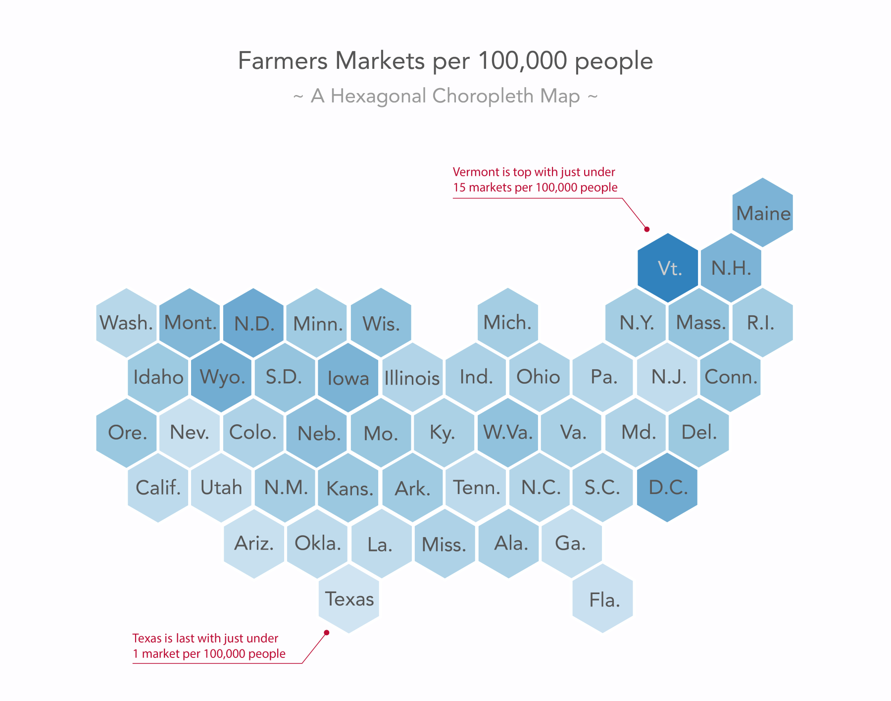
Let's be clear, hexagons in a hexbin map as described in the preceding diagram and in the following sections represent equal areas. Hexagons in a hexagonal choropleth map as shown in this figure represent vastly different areas. However, in this case, we don’t want to focus on the spatial area of our chosen unit (US mainland states); we want to focus on the measure that is merely categorized by our chosen unit.

Be aware that this comes with the cost of removing the area information entirely, as the US states differ greatly in area and no state looks like a hexagon. However, unlike the preceding classic choropleth example, this hexagonal choropleth allows us, for example, to easily identify Washington D.C. as a farmers' market hub and that might be the message we want to bring across above all.

Enough theory. Let’s make a hexbin map.