Table of Contents for
QGIS: Becoming a GIS Power User
 QGIS: Becoming a GIS Power User
Published by
Packt Publishing, 2017
QGIS: Becoming a GIS Power User
Published by
Packt Publishing, 2017
- Cover
- Table of Contents
- QGIS: Becoming a GIS Power User
- QGIS: Becoming a GIS Power User
- QGIS: Becoming a GIS Power User
- Credits
- Preface
- What you need for this learning path
- Who this learning path is for
- Reader feedback
- Customer support
- 1. Module 1
- 1. Getting Started with QGIS
- Running QGIS for the first time
- Introducing the QGIS user interface
- Finding help and reporting issues
- Summary
- 2. Viewing Spatial Data
- Dealing with coordinate reference systems
- Loading raster files
- Loading data from databases
- Loading data from OGC web services
- Styling raster layers
- Styling vector layers
- Loading background maps
- Dealing with project files
- Summary
- 3. Data Creation and Editing
- Working with feature selection tools
- Editing vector geometries
- Using measuring tools
- Editing attributes
- Reprojecting and converting vector and raster data
- Joining tabular data
- Using temporary scratch layers
- Checking for topological errors and fixing them
- Adding data to spatial databases
- Summary
- 4. Spatial Analysis
- Combining raster and vector data
- Vector and raster analysis with Processing
- Leveraging the power of spatial databases
- Summary
- 5. Creating Great Maps
- Labeling
- Designing print maps
- Presenting your maps online
- Summary
- 6. Extending QGIS with Python
- Getting to know the Python Console
- Creating custom geoprocessing scripts using Python
- Developing your first plugin
- Summary
- 2. Module 2
- 1. Exploring Places – from Concept to Interface
- Acquiring data for geospatial applications
- Visualizing GIS data
- The basemap
- Summary
- 2. Identifying the Best Places
- Raster analysis
- Publishing the results as a web application
- Summary
- 3. Discovering Physical Relationships
- Spatial join for a performant operational layer interaction
- The CartoDB platform
- Leaflet and an external API: CartoDB SQL
- Summary
- 4. Finding the Best Way to Get There
- OpenStreetMap data for topology
- Database importing and topological relationships
- Creating the travel time isochron polygons
- Generating the shortest paths for all students
- Web applications – creating safe corridors
- Summary
- 5. Demonstrating Change
- TopoJSON
- The D3 data visualization library
- Summary
- 6. Estimating Unknown Values
- Interpolated model values
- A dynamic web application – OpenLayers AJAX with Python and SpatiaLite
- Summary
- 7. Mapping for Enterprises and Communities
- The cartographic rendering of geospatial data – MBTiles and UTFGrid
- Interacting with Mapbox services
- Putting it all together
- Going further – local MBTiles hosting with TileStream
- Summary
- 3. Module 3
- 1. Data Input and Output
- Finding geospatial data on your computer
- Describing data sources
- Importing data from text files
- Importing KML/KMZ files
- Importing DXF/DWG files
- Opening a NetCDF file
- Saving a vector layer
- Saving a raster layer
- Reprojecting a layer
- Batch format conversion
- Batch reprojection
- Loading vector layers into SpatiaLite
- Loading vector layers into PostGIS
- 2. Data Management
- Joining layer data
- Cleaning up the attribute table
- Configuring relations
- Joining tables in databases
- Creating views in SpatiaLite
- Creating views in PostGIS
- Creating spatial indexes
- Georeferencing rasters
- Georeferencing vector layers
- Creating raster overviews (pyramids)
- Building virtual rasters (catalogs)
- 3. Common Data Preprocessing Steps
- Converting points to lines to polygons and back – QGIS
- Converting points to lines to polygons and back – SpatiaLite
- Converting points to lines to polygons and back – PostGIS
- Cropping rasters
- Clipping vectors
- Extracting vectors
- Converting rasters to vectors
- Converting vectors to rasters
- Building DateTime strings
- Geotagging photos
- 4. Data Exploration
- Listing unique values in a column
- Exploring numeric value distribution in a column
- Exploring spatiotemporal vector data using Time Manager
- Creating animations using Time Manager
- Designing time-dependent styles
- Loading BaseMaps with the QuickMapServices plugin
- Loading BaseMaps with the OpenLayers plugin
- Viewing geotagged photos
- 5. Classic Vector Analysis
- Selecting optimum sites
- Dasymetric mapping
- Calculating regional statistics
- Estimating density heatmaps
- Estimating values based on samples
- 6. Network Analysis
- Creating a simple routing network
- Calculating the shortest paths using the Road graph plugin
- Routing with one-way streets in the Road graph plugin
- Calculating the shortest paths with the QGIS network analysis library
- Routing point sequences
- Automating multiple route computation using batch processing
- Matching points to the nearest line
- Creating a routing network for pgRouting
- Visualizing the pgRouting results in QGIS
- Using the pgRoutingLayer plugin for convenience
- Getting network data from the OSM
- 7. Raster Analysis I
- Using the raster calculator
- Preparing elevation data
- Calculating a slope
- Calculating a hillshade layer
- Analyzing hydrology
- Calculating a topographic index
- Automating analysis tasks using the graphical modeler
- 8. Raster Analysis II
- Calculating NDVI
- Handling null values
- Setting extents with masks
- Sampling a raster layer
- Visualizing multispectral layers
- Modifying and reclassifying values in raster layers
- Performing supervised classification of raster layers
- 9. QGIS and the Web
- Using web services
- Using WFS and WFS-T
- Searching CSW
- Using WMS and WMS Tiles
- Using WCS
- Using GDAL
- Serving web maps with the QGIS server
- Scale-dependent rendering
- Hooking up web clients
- Managing GeoServer from QGIS
- 10. Cartography Tips
- Using Rule Based Rendering
- Handling transparencies
- Understanding the feature and layer blending modes
- Saving and loading styles
- Configuring data-defined labels
- Creating custom SVG graphics
- Making pretty graticules in any projection
- Making useful graticules in printed maps
- Creating a map series using Atlas
- 11. Extending QGIS
- Defining custom projections
- Working near the dateline
- Working offline
- Using the QspatiaLite plugin
- Adding plugins with Python dependencies
- Using the Python console
- Writing Processing algorithms
- Writing QGIS plugins
- Using external tools
- 12. Up and Coming
- Preparing LiDAR data
- Opening File Geodatabases with the OpenFileGDB driver
- Using Geopackages
- The PostGIS Topology Editor plugin
- The Topology Checker plugin
- GRASS Topology tools
- Hunting for bugs
- Reporting bugs
- Bibliography
- Index
You can extend the capabilities of QGIS by adding scripts that can be used within the Processing framework. This will allow you to create your own analysis algorithms and then run them efficiently from the toolbox or from any of the productivity tools, such as the batch processing interface or the graphical modeler.
This recipe covers basic ideas about how to create a Processing algorithm.
A basic knowledge of Python is needed to understand this recipe. Also, as it uses the Processing framework, you should be familiar with it before studying this recipe.
We are going to add a new process to filter the polygons of a layer, generating a new layer that just contains the ones with an area larger than a given value. Here's how to do this:
- In the Processing Toolbox menu, go to the Scripts/Tools group and double-click on the Create new script item. You will see the following dialog:
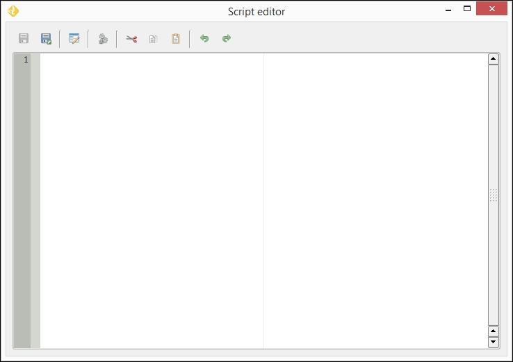
- In the text editor of the dialog, paste the following code:
##Cookbook=group ##Filter polygons by size=name ##Vector_layer=vector ##Area=number 1 ##Output=output vector layer = processing.getObject(Vector_layer) provider = layer.dataProvider() writer = processing.VectorWriter(Output, None, provider.fields(), provider.geometryType(), layer.crs()) for feature in processing.features(layer): print feature.geometry().area() if feature.geometry().area() > Area: writer.addFeature(feature) del writer - Select the Save button to save the script. In the file selector that will appear, enter a filename with the
.pyextension. Do not move this to a different folder. Make sure that you use the default folder that is selected when the file selector is opened. - Close the editor.
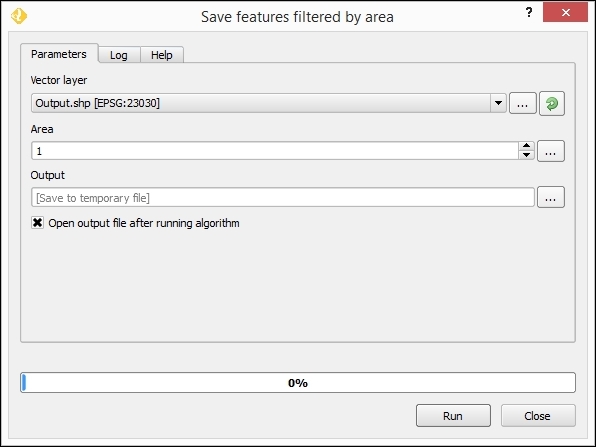
- Go to the Scripts groups in the toolbox, and you will see a new group called Cookbook with an algorithm called
Filter polygons by size. - Double-click on it to open it, and you will see the following parameters dialog, similar to what you can find for any of the other Processing algorithms:
The script contains mainly two parts:
- A part in which the characteristics of the algorithm are defined. This is used to define the semantics of the algorithm, along with some additional information, such as the name and group of the algorithm.
- A part that takes the inputs entered by the user and processes them to generate the outputs. This is where the algorithm itself is located.
In our example, the first part looks like the following:
##Cookbook=group
##Filter polygons by size=name
##Vector_layer=vector
##Area=number 1
##Output=output vector
We are defining two inputs (the layer and the area value) and declaring one output (the filtered layer). These elements are defined using the Python comments with a double Python comment sign (#).
The second part includes the code itself and looks like the following:
layer = processing.getObject(Vector_layer)
provider = layer.dataProvider()
writer = processing.VectorWriter(Output, None,
  provider.fields(), provider.geometryType(), layer.crs())
for feature in processing.features(layer):
  print feature.geometry().area()
  if feature.geometry().area() > Area:
    writer.addFeature(feature)
del writer
The inputs that we defined in the first part will be available here, and we can use them. In the case of the area, we will have a variable named Area, containing a number. In the case of the vector layer, we will have a Layer variable, containing a string with the source of the selected layer.
Using these values, we use the PyQGIS API to perform the calculations and create a new layer. The layer is saved in the file path contained in the Output variable, which is the one that the user will select when running the algorithm.
Apart from using regular Python and the PyQGIS interface, Processing includes some classes and functions because this makes it easier to create scripts, and that wrap some of the most common functionality of QGIS.
In particular, the processing.features(layer) method is important. This provides an iterator over the features in a layer, but only considering the selected ones. If no selection exists, it iterates over all the features in the layer. This is the expected behavior of any Processing algorithm, so this method has to be used to provide a consistent behavior in your script.
Some of the core algorithms that are provided with Processing are actually scripts, such as the one we just created, but they do not appear in the scripts section. Instead, they appear in the QGIS algorithms section because they are a core part of Processing.
Other scripts are not part of processing itself but they can be installed easily from the toolbox using the Tools/Get scripts from on-line collection menu:
You will see a window like the following one:
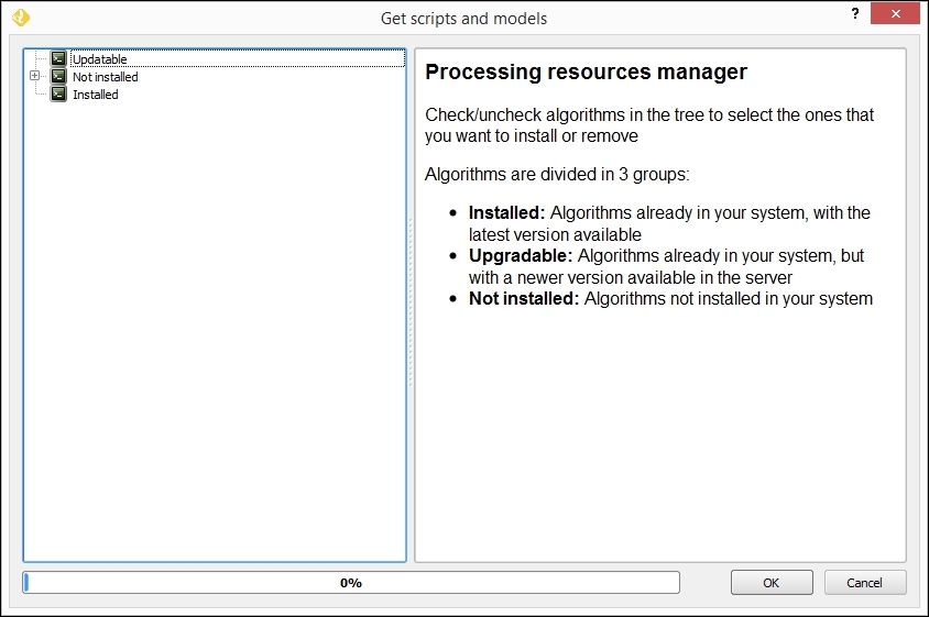
Just select the scripts that you want to install and then click on OK. The selected scripts will now appear in the toolbox. You can use it as you use any other Processing algorithm.