The basemap

In web map applications, the meaning of basemap sometimes differs from that in use for print maps; basemaps are the unchanging, often cached, layers of the map visualization that tend to appear behind the layers that support interaction. In our example, the basemap could be the georeferenced historical image, alone or with other layers.

You should consider using a public basemap service if one is suitable for your project. You can browse a selection of these in QGIS using the OpenLayers plugin.

Tip

Use a basemap service if the following conditions are fulfilled:

The geographic features provide adequate context for your operational layer(s)
The extent is suitable for your map interface
Scale levels are suitable for your map interface, particularly smallest and largest
Basemap labels and symbols don't obscure your operational layer(s)
The map service provides terms of use consistent with your intended use
You do not need to be able to view the basemap when disconnected from the internet

If our basemap were not available via a web service as in our example, we must turn our attention to its production. It is important to consider what a basemap is and how it differs from the operational layer.

The geographic reference features included in a basemap are selected according to the map's intended use and audience. Often, this includes certain borders, roads, topography, hydrography, and so on.

Tip

Beyond these reference features, include the geographic object class in the basemap if you do not need:

To regularly update the geometric data
To provide capabilities for style changes
To permit visibility change in class objects independently of other data
To expose objects in the class to interface controls

Assuming that we will be using some kind of caching mechanism to store and deliver the basemap, we will optimize performance by maximizing the objects included therein.

Using OpenStreetMap for the basemap data

Obtaining data for a basemap is not a trivial task. If a suitable map service is available via a web service, it would ease the task considerably. Otherwise, you must obtain supporting data from your local system and render this to a suitable cartographic format.

A challenge in creating basemaps and keeping them updated is interacting with different data providers. Different organizations tend be recognized as the provider of choice for the different classes of geographic objects. With different organizations in the mix, different data format conventions are bound to occur.

OpenStreetMap (OSM), an open data repository for geographic reference data, provides both map services and data. In addition to OSM's own map services, the data repository is a source for a number of other projects offering free basemap services.

OpenStreetMap uses a more abstract and scalable schema than most data providers. The OSM data includes a few system fields, such as osm_id, user_id, osm_version, and way. The osm_id field is unique to each geographic object, user_id is unique to the user who last modified the object, osm_version is unique to the versions for the object, and way is the geometry of the object.

By allowing a theoretically unlimited number of key value pairs along with the system fields mentioned before, the OSM data schema can potentially allow any kind of data and still maintain sanity. Keys are whatever the data editors add to the data that they upload to the repository. The well-established keys are documented on the OSM site and are compatible with the community produced rendering styles. If a community produced style does not include the key that you need or the one that you created, you can simply add it into your own rendering style. Columns are kept from overwhelming a local database during the import stage. Only keys added in a local configuration file are added to the database schema and populated.

High quality cartography with OSM data is an ongoing challenge. CloudMade has created its business on a cloud-based, albeit limited, rendering editor for OSM data, which is capable of also serving map services. CloudMade is, in fact, a fine source for cloud services for OSM data and has many visually appealing styles available. OpenMapSurfer, produced by a research group at the University of Heidelberg, shows off some best practices in high quality cartography with OSM data including sophisticated label placement, object-level scale dependency, careful color selection, and shaded topographic relief and bathymetry.

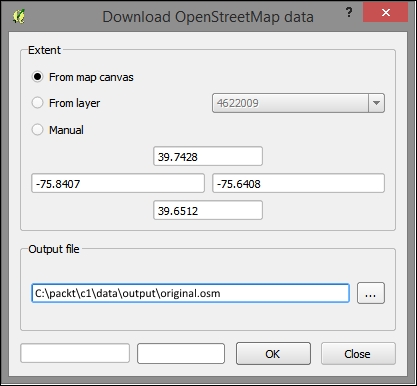
To obtain the OpenStreetMap data locally to produce your own basemap, perform the following steps:

Install the OpenLayers and OSMDownloader QGIS plugins if they are not already installed.
Create a new SpatiaLite database.
Turn on OSM:
1. Navigate to Web | OpenLayers | OpenStreetMap | OpenStreetMap.
Browse your area of interest.
Download your area of interest:
1. Navigate to Vector | OpenStreetMap | Download Data:
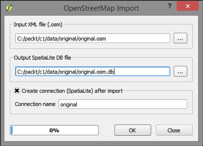
Import the downloaded XML data into a topological SQLite database. This does not contain SpatiaLite geographic objects; rather, it is expressed in terms of topological relationships between objects in a table. Topological relationships are explored in more depth in Chapter 4, Finding the Best Way to Get There, and Chapter 5, Demonstrating Change.
1. Navigate to Vector | OpenStreetMap | Import Topology from XML.
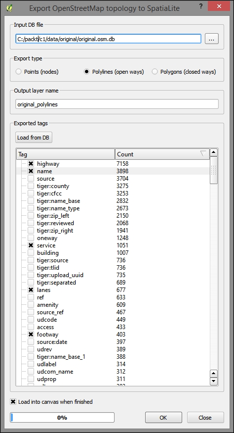
Convert topology to SpatiaLite spatial tables through the following steps:
1. Navigate to Vector | OpenStreetMap | Export Topology to Spatialite.
2. Select the points, polylines, or polygons to export.
3. Then, select the fields that you may want to use for styling purposes. You can populate a list of possible fields by clicking on Load from DB.
4. You can repeat this step to export the additional geometry types, as shown in the following screenshot:
You can now style this as you like and export it as the tiled basemap. Then, you can save it in the mapnik or sld style for use in rendering in an external tile caching software.

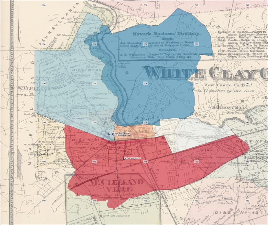
Here's an example of the OSM data overlaid on our other layers with a basic, single symbol style:

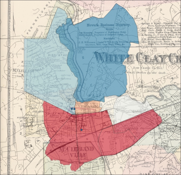
Using OpenStreetMap for the basemap data

Avoiding obscurity and confusion

Of course, heaping data in the basemap is not without its drawbacks. Other than the relative loss of functionality, which occurs by design, basemaps can quickly become cluttered and otherwise unclear. The layer and label scale dependency dynamically alter the display of information to avoid the obfuscation of basemap geographic classes.

The layer scale dependency

When classes of geographic objects are unnecessary to visualize at certain scales, the whole layer scale dependency can be used to hide the layer from view. For example, in the preceding image, we can see all the layers, including the geocoded addresses, at a smaller scale even when they may not be distinctly visible. To simplify the information, we can apply the layer scale dependency so that this layer does not show these small scales.

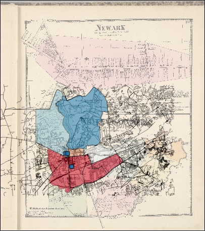
At this scale, some objects are not distinctly visible. Using the layer scale dependency, we can make these objects invisible at this scale.

It is also possible to alter visibility with scale at the geographic object level within a layer. For example, you may wish to show only the major roads at a small scale. However, this will generally require more effort to produce. Object-level visibility can be driven by attributes already existing or created for the purpose of scale dependency. It can also be defined according to the geometric characteristics of an object, such as its area. In general, smaller features should not be viewable at lower scales.

A common way to achieve layer dependency at the object level using the whole-layer dependency is to select objects that match the given criteria and create new layers from these. Scale dependency can be applied to the subsets of the object class now contained in this separate layer.

You will want to set the layer scale dependency in accordance with scale ratios that conform to those that are commonly used. These are based on some assumptions, including those about the resolution of the tiled image (96 dpi) and the size of the tile (256px x 265px).

Zoom	Object extent	Scale at 96 dpi
`0`	Entire planet	`1 : 59165752759.16`
`1`		`1 : 295,829,355.45`
`2`		`1 : 147,914,677.73`
`3`		`1 : 73,957,338.86`
`4`		`1 : 36,978,669.43`
`5`	Country	`1 : 18,489,334.72`
`6`		`1 : 9,244,667.36`
`7`		`1 : 4,622,333.68`
`8`	State	`1 : 2,311,166.84`
`9`		`1 : 1,155,583.42`
`10`	Metropolitan	`1 : 577,791.71`
`11`		`1 : 288,895.85`
`12`	City	`1 : 144,447.93`
`13`		`1 : 72,223.96`
`14`	Town	`1 : 36,111.98`
`15`		`1 : 18,055.99`
`16`	Minor road	`1 : 9,028.00`
`17`		`1 : 4,514.00`
`18`	Sidewalks	`1 : 2,257.00`

The label conflict

Labels are commonly separated from the basemap layer itself. One reason for this is that if labels are included in the basemap layer, they will be obscured by the operational layer displayed above it. Another reason is that tile caching sometimes does not properly handle labels, causing fragments of labels to be left missing. Labels should also be displayed with their own scale dependency, filtering out only the most important labels at smaller scales. If you have many layers and objects to be labeled, this may be a good use case for a map server or at least a rendering engine such as Mapnik.

The polygon label conflict resolution

To achieve conflict resolution between label layers on our map output, we will convert the geographic objects to be labeled to centroids—points in the middle of each object—which will then be displayed along with the label field as a label layer.

Convert objects to points through the following steps:
1. Navigate to Vector | Geometry Tools | Polygon Centroids.
2. If the polygons are in a database, create an SQL view where the polygons are stored, as shown in the following code:
```
CREATE VIEW AS 
SELECT polygon_class.label, st_centroid(polygon_class.geography) AS geography
  FROM polygon_class;
```
Create a layer corresponding to the labels in the map server or renderer.
Add any adjustments via the SLD or whichever style markup you will use. The GeoServer implementation is particularly good at resolving conflicts and improving placement.

Chapter 7, Mapping for Enterprises and Communities, includes a more detailed blueprint for creating a labeling layer with a cartographically enhanced placement and conflict resolution using SLD in GeoServer.

The characteristics of the basemap will affect the range of interaction, panning, and zooming in the map interface. You will want a basemap that covers the extent of the area to be seen on the map interface and probably restrict the interface to a region of interest. This way, someone viewing a collection of buildings in a corner of one state does not get lost panning to the opposite corner of another state! When you cache your basemap, you will want to indicate that you wish to cache to this extent. Similarly, viewable scales will be configured at the time your basemap is cached, and you'll want to indicate which these are. This affects the incremental steps, in which the zoom tool increases or decreases the map scale.

Tile caches

The best way to cache your basemap data so that it quickly loads is to save it as individual images. Rather than requiring a potentially complicated rendering by the browser of many geometric features, a few images corresponding to the scale and extent to which they are viewed can be quickly transferred from client to server and displayed. These prerendered images are referred to as tiles because these square images will be displayed seamlessly when the basemap is requested. This is now the standard method used to prepare data for web mapping. In this book, we will cover two tools to create tile caches: QTiles plugin (Chapter 1, Exploring Places – from Concept to Interface) and TileMill/MBTiles (Chapter 7, Mapping for Enterprises and Communities).

	Configuration time	Execution time	Visual quality	Stored in a single file	Stored as image directories	Suitable for labels
QTiles Plugin	1	3	3	No	Yes	No
GDAL2Tiles.py	2	1	2	No	Yes	No
TileMill/MBTiles	3	2	1	Yes	No	Yes
GeoServer/GWC	3	2	1	No	No	Yes

You will need to pay some attention to the scheme for tile storage that is used. The .mbtiles format that TileMill uses is a SQLite database that will need to be read with a map interface that supports it, such as Leaflet. The QTiles plugin and GDAL2Tiles.py use an XYZ tile scheme with hierarchical directories based on row (X), column (Y), and zoom (Z) respectively with the origin in the top-left corner of the map. This is the most popular tiling scheme. The TMS tiling scheme sometimes used by GeoServer open source map server (which supports multiple schemes/service specifications) and that accepted by OSGeo are almost identical; however, the origin is at the bottom-left of the map. This often leads to some confusing results. Note that zoom levels are standardized according to the tile scheme tile size and resolution (for example, 256 x 256 pixels)

Generating and testing a simple directory-based tile cache structure

We will now use the QTiles plugin to generate a directory-based ZYX tile scheme cache. Perform the following steps:

Install QTiles and the TileLayer plugin.
- QTiles is listed under the experimental plugins. You must alter the plugin settings to show experimental plugins. Navigate to Plugins | Manage and Install Plugins | Settings | "Show also experimental plugins".
Run QTiles, creating a new mytiles tileset with a minimum zoom of 14 and maximum of 16.
You'll realize the value of this directory in the next example.
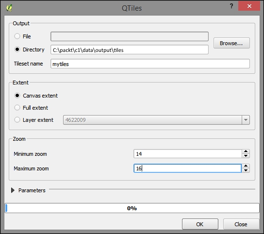
You can test and see whether the tiles were created by looking under the directory where you created them. They will be under the directory in the numbered subdirectories given by their Z, X, and Y grid positions in the tiling scheme. For example, here's a tile at 15/9489/12442.png. That's 15 zoom, 9489 longitude in the grid scheme, and 12442 latitude in the grid scheme.

You will now see the following output:

Generating and testing a simple directory-based tile cache structure

Create a layer description file for the TileLayer plugin

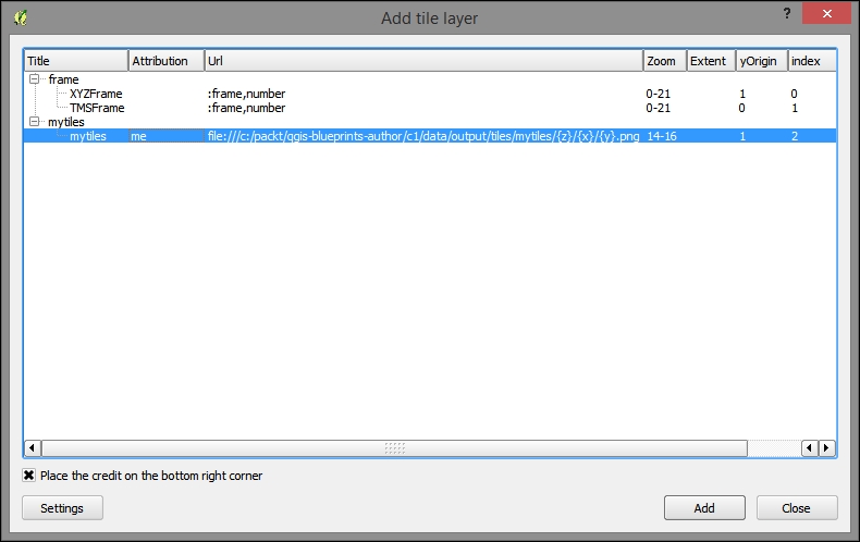
Create a layer description file with a tsv (tab delimited) extension in the UTF-8 encoding. This is a universal text encoding that is widely used on the Web and is sometimes needed for compatibility.

Note

Note that the last six parameters are optional and may prevent missing tiles. In the following example, I will use only the z parameters, zmin and zmax, related to map zoom level.

Add text in the following form, containing all tile parameters, to a new file:
```
title credit url yOriginTop [zmin zmax xmin ymin xmax ymax]
```
- For example, mytiles me file:///c:/packt/c1/data/output/tiles/ mytiles/{z}/{x}/{y}.png 1 14 16.
- In the preceding example, the description file refers to a local Windows file system path, where the tiled .png images are stored.
Save mytiles.tsv to the following path:
```
[YOUR HOME DIRECTORY]/.qgis2///python/plugins/TileLayerPlugin/layers
```
- For me, on Windows, this was C:\Users\[user]\.qgis2\python\plugins\TileLayerPlugin\layers.
  Note
  Note that .qgis2 may be a hidden directory on some systems. Make sure to show the hidden directories/files.
- The path for the location to save your TSV file can be found or set under Web | TileLayer Plugin | Add Tile Layer | Settings | External layer definition directory.

Preview it with the TileLayer plugin. You should be able to add the layer from the TilerLayerPlugin dialog. Now that the layer description file has been added to the correct location, let's go to Web TileLayerPlugin | Add Tile Layer: