Editing attributes

There are three main use cases of attribute editing:

First, we might want to edit the attributes of a specific feature, for example, to fix a wrong name
Second, we might want to edit the attributes of a group of features
Third, we might want to change the attributes of all features within a layer

Editing attributes in the attribute table

All three use cases are covered by the functionality available through the attribute table. We can access it by going to Layer | Open Attribute Table, using the Open Attribute Table button present in the Attributes toolbar, or in the layer name context menu.

To change an attribute value, we always have to enable editing first.
Then, we can double-click on any cell in the attribute table to activate the input mode, as shown in the upper dialog of the following screenshot, where I am editing NAME_2 of the first feature: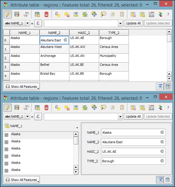
Pressing the Enter key confirms the change, but to save the new value permanently, we also have to click on the Save Edit(s) button or press Ctrl + S.

Besides the classic attribute table view, QGIS also supports a form view, which you can see in the lower dialog of the previous image. You can switch between these two views using the buttons in the bottom-right corner of the attribute table dialog.

Tip

In the attribute table, we also find tools for handling selections (from left to right, starting at the fourth button): Delete selected features, Select features using an expression, Unselect all, Move selection to top, Invert selection, Pan map to the selected rows, Zoom map to the selected rows, and Copy selected rows to clipboard. Another way to select features in the attribute table is by clicking on the row number.

The next two buttons allow us to add and remove columns. When we click on the Delete column button, we get a list of columns to choose from. Similarly, the New column button brings up a dialog that we can use to specify the name and data type of the new column.

Editing attributes in the feature form

Another option to edit the attributes of one feature is to open the attribute form directly by clicking on the feature on the map using the Identify tool. By default, the Identify tool displays the attribute values in read mode, but we can enable the Auto open form option in the Identify Results panel, as shown here:

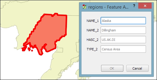
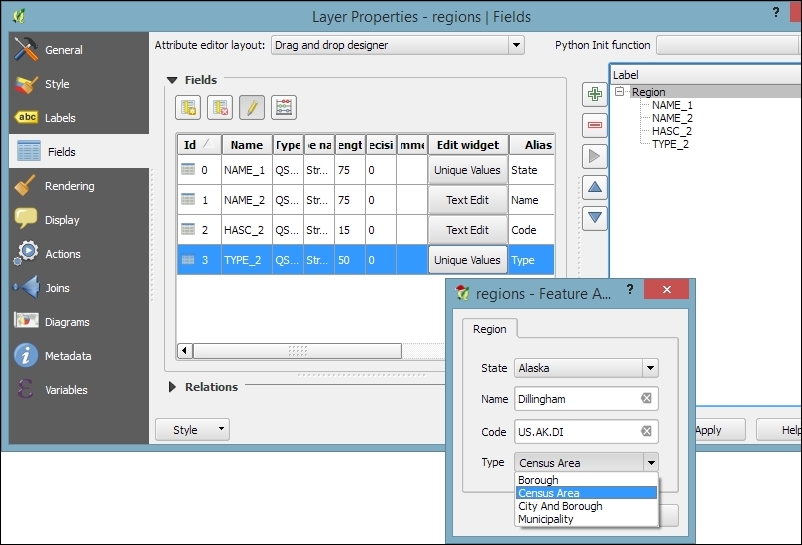
What you can see in the previous screenshot is the default feature attributes form that QGIS creates automatically, but we are not limited to this basic form. By going to Layer Properties | Fields section, we can configure the look and feel of the form in greater detail. The Attribute editor layout options are (in an increasing level of complexity) autogenerate, Drag and drop designer, and providing a .ui file. These options are described in detail as follows.

Creating a feature form using autogenerate

Autogenerate is the most basic option. You can assign a specific Edit widget and Alias for each field; this will replace the default input field and label in the form. For this example, we use the following edit widget types:

Text Edit supports inserting one or more lines of text.
Unique Values creates a drop-down list that allows the user to select one of the values that have already been used in the attribute table. If the Editable option is activated, the drop-down list is replaced by a text edit widget with autocompletion support.
Range creates an edit widget for numerical values from a specific range.

Note

For the complete list of available Edit widget types, refer to the user manual at http://docs.qgis.org/2.2/en/docs/user_manual/working_with_vector/vector_properties.html#fields-menu.

Designing a feature form using drag and drop designer

This allows more control over the form layout. As you can see in the next screenshot, the designer enables us to create tabs within the form and also makes it possible to change the order of the form fields. The workflow is as follows:

Click on the plus button to add one or more tabs (for example, a Region tab, as shown in the following screenshot).
On the left-hand side of the dialog, select the field that you want to add to the form.
On the right-hand side, select the tab to which you want to add the field.
Click on the button with the icon of an arrow pointing to the right to add the selected field to the selected tab.
You can reorder the fields in the form using the up and down arrow buttons or, as the name suggests, by dragging and dropping the fields up or down:

Designing a feature form using a .ui file

This is the most advanced option. It enables you to use a Qt user interface designed using, for example, the Qt Designer software. This allows a great deal of freedom in designing the form layout and behavior.

Note

Creating .ui files is out of the scope of this book, but you can find more information about it at http://docs.qgis.org/2.2/en/docs/training_manual/create_vector_data/forms.html#hard-fa-creating-a-new-form.

Calculating new attribute values

If we want to change the attributes of multiple or all features in a layer, editing them manually usually isn't an option. This is what the Field calculator is good for. We can access it using the Open field calculator button in the attribute table, or by pressing Ctrl + I. In the Field calculator, we can choose to update only the selected features or update all the features in the layer. Besides updating an existing field, we can also create a new field. The function list is the same one that we explored when we selected features by expression. We can use any of the functions and variables in this list to populate a new field or update an existing one. Here are some example expressions that are often used:

We can create a sequential id column using the @row_number variable, which populates a column with row numbers, as shown in the following screenshot: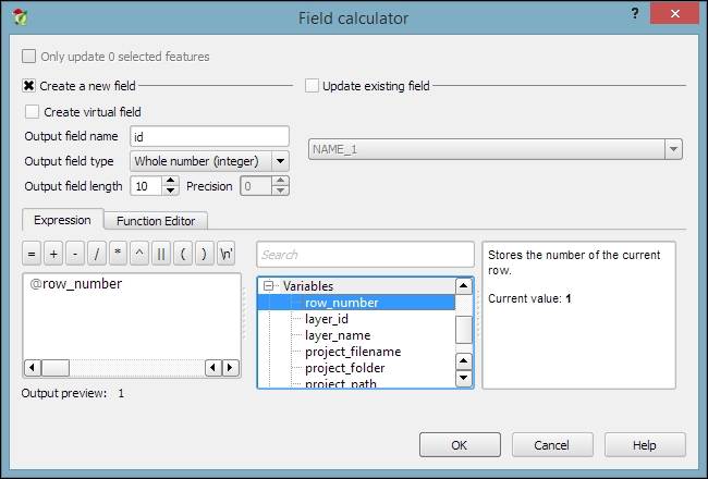
Another common use case is calculating a line's length or a polygon's area using the $length and $area geometry functions, respectively
Similarly, we can get point coordinates using $x and $y
If we want to get the start point or end point of a line, we can use $x_at(0) and $y_at(0), or $x_at(-1) and $y_at(-1), respectively

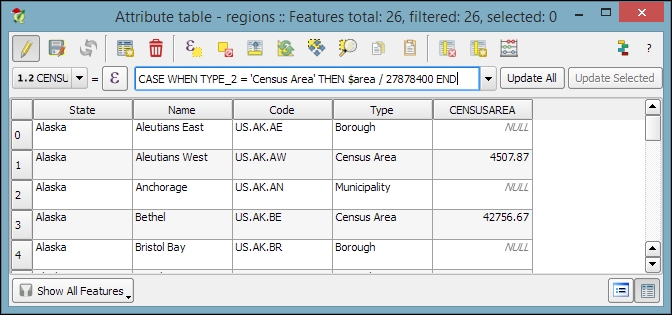
An alternative to the Field calculator—especially if you already know the formula you want to use—is the field calculator bar, which you can find directly in the Attribute table dialog right below the toolbar. In the next screenshot, you can see an example that calculates the area of all census areas (use the New Field button to add a Decimal number field called CENSUSAREA first). This example uses a CASE WHEN – THEN – END expression to check whether the value of TYPE_2 is Census Area:

CASE WHEN TYPE_2 = 'Census Area' THEN $area / 27878400 END

Tip

An alternative solution would be to use the if() function instead. If you use the CENSUSAREA attribute as the third parameter (which defines the value that is returned if the condition evaluates to false), the expression will only update those rows in which TYPE_2 is Census Area and leave the other rows unchanged:

if(TYPE_2 = 'Census Area', $area / 27878400, CENSUSAREA)

Alternatively, you can use NULL as a third parameter which will overwrite all rows where TYPE_2 does not equal Census Area with NULL:

if(TYPE_2 = 'Census Area', $area / 27878400, NULL)

Enter the formula and click on the Update All button to execute it:

Since it is not possible to directly change a field data type in a Shapefile or SpatiaLite attribute table, the field calculator and calculator bar are also used to create new fields with the desired properties and then populate them with the values from the original column.

Previous Chapter

Using measuring tools

Next Chapter

Reprojecting and converting vector and raster data

Table of Contents for QGIS: Becoming a GIS Power User

Editing attributes

Editing attributes in the attribute table

Tip

Editing attributes in the feature form

Creating a feature form using autogenerate

Note

Designing a feature form using drag and drop designer

Designing a feature form using a .ui file

Note

Calculating new attribute values

Tip

Table of Contents for
QGIS: Becoming a GIS Power User