Table of Contents for
QGIS: Becoming a GIS Power User
 QGIS: Becoming a GIS Power User
Published by
Packt Publishing, 2017
QGIS: Becoming a GIS Power User
Published by
Packt Publishing, 2017
- Cover
- Table of Contents
- QGIS: Becoming a GIS Power User
- QGIS: Becoming a GIS Power User
- QGIS: Becoming a GIS Power User
- Credits
- Preface
- What you need for this learning path
- Who this learning path is for
- Reader feedback
- Customer support
- 1. Module 1
- 1. Getting Started with QGIS
- Running QGIS for the first time
- Introducing the QGIS user interface
- Finding help and reporting issues
- Summary
- 2. Viewing Spatial Data
- Dealing with coordinate reference systems
- Loading raster files
- Loading data from databases
- Loading data from OGC web services
- Styling raster layers
- Styling vector layers
- Loading background maps
- Dealing with project files
- Summary
- 3. Data Creation and Editing
- Working with feature selection tools
- Editing vector geometries
- Using measuring tools
- Editing attributes
- Reprojecting and converting vector and raster data
- Joining tabular data
- Using temporary scratch layers
- Checking for topological errors and fixing them
- Adding data to spatial databases
- Summary
- 4. Spatial Analysis
- Combining raster and vector data
- Vector and raster analysis with Processing
- Leveraging the power of spatial databases
- Summary
- 5. Creating Great Maps
- Labeling
- Designing print maps
- Presenting your maps online
- Summary
- 6. Extending QGIS with Python
- Getting to know the Python Console
- Creating custom geoprocessing scripts using Python
- Developing your first plugin
- Summary
- 2. Module 2
- 1. Exploring Places – from Concept to Interface
- Acquiring data for geospatial applications
- Visualizing GIS data
- The basemap
- Summary
- 2. Identifying the Best Places
- Raster analysis
- Publishing the results as a web application
- Summary
- 3. Discovering Physical Relationships
- Spatial join for a performant operational layer interaction
- The CartoDB platform
- Leaflet and an external API: CartoDB SQL
- Summary
- 4. Finding the Best Way to Get There
- OpenStreetMap data for topology
- Database importing and topological relationships
- Creating the travel time isochron polygons
- Generating the shortest paths for all students
- Web applications – creating safe corridors
- Summary
- 5. Demonstrating Change
- TopoJSON
- The D3 data visualization library
- Summary
- 6. Estimating Unknown Values
- Interpolated model values
- A dynamic web application – OpenLayers AJAX with Python and SpatiaLite
- Summary
- 7. Mapping for Enterprises and Communities
- The cartographic rendering of geospatial data – MBTiles and UTFGrid
- Interacting with Mapbox services
- Putting it all together
- Going further – local MBTiles hosting with TileStream
- Summary
- 3. Module 3
- 1. Data Input and Output
- Finding geospatial data on your computer
- Describing data sources
- Importing data from text files
- Importing KML/KMZ files
- Importing DXF/DWG files
- Opening a NetCDF file
- Saving a vector layer
- Saving a raster layer
- Reprojecting a layer
- Batch format conversion
- Batch reprojection
- Loading vector layers into SpatiaLite
- Loading vector layers into PostGIS
- 2. Data Management
- Joining layer data
- Cleaning up the attribute table
- Configuring relations
- Joining tables in databases
- Creating views in SpatiaLite
- Creating views in PostGIS
- Creating spatial indexes
- Georeferencing rasters
- Georeferencing vector layers
- Creating raster overviews (pyramids)
- Building virtual rasters (catalogs)
- 3. Common Data Preprocessing Steps
- Converting points to lines to polygons and back – QGIS
- Converting points to lines to polygons and back – SpatiaLite
- Converting points to lines to polygons and back – PostGIS
- Cropping rasters
- Clipping vectors
- Extracting vectors
- Converting rasters to vectors
- Converting vectors to rasters
- Building DateTime strings
- Geotagging photos
- 4. Data Exploration
- Listing unique values in a column
- Exploring numeric value distribution in a column
- Exploring spatiotemporal vector data using Time Manager
- Creating animations using Time Manager
- Designing time-dependent styles
- Loading BaseMaps with the QuickMapServices plugin
- Loading BaseMaps with the OpenLayers plugin
- Viewing geotagged photos
- 5. Classic Vector Analysis
- Selecting optimum sites
- Dasymetric mapping
- Calculating regional statistics
- Estimating density heatmaps
- Estimating values based on samples
- 6. Network Analysis
- Creating a simple routing network
- Calculating the shortest paths using the Road graph plugin
- Routing with one-way streets in the Road graph plugin
- Calculating the shortest paths with the QGIS network analysis library
- Routing point sequences
- Automating multiple route computation using batch processing
- Matching points to the nearest line
- Creating a routing network for pgRouting
- Visualizing the pgRouting results in QGIS
- Using the pgRoutingLayer plugin for convenience
- Getting network data from the OSM
- 7. Raster Analysis I
- Using the raster calculator
- Preparing elevation data
- Calculating a slope
- Calculating a hillshade layer
- Analyzing hydrology
- Calculating a topographic index
- Automating analysis tasks using the graphical modeler
- 8. Raster Analysis II
- Calculating NDVI
- Handling null values
- Setting extents with masks
- Sampling a raster layer
- Visualizing multispectral layers
- Modifying and reclassifying values in raster layers
- Performing supervised classification of raster layers
- 9. QGIS and the Web
- Using web services
- Using WFS and WFS-T
- Searching CSW
- Using WMS and WMS Tiles
- Using WCS
- Using GDAL
- Serving web maps with the QGIS server
- Scale-dependent rendering
- Hooking up web clients
- Managing GeoServer from QGIS
- 10. Cartography Tips
- Using Rule Based Rendering
- Handling transparencies
- Understanding the feature and layer blending modes
- Saving and loading styles
- Configuring data-defined labels
- Creating custom SVG graphics
- Making pretty graticules in any projection
- Making useful graticules in printed maps
- Creating a map series using Atlas
- 11. Extending QGIS
- Defining custom projections
- Working near the dateline
- Working offline
- Using the QspatiaLite plugin
- Adding plugins with Python dependencies
- Using the Python console
- Writing Processing algorithms
- Writing QGIS plugins
- Using external tools
- 12. Up and Coming
- Preparing LiDAR data
- Opening File Geodatabases with the OpenFileGDB driver
- Using Geopackages
- The PostGIS Topology Editor plugin
- The Topology Checker plugin
- GRASS Topology tools
- Hunting for bugs
- Reporting bugs
- Bibliography
- Index
In this chapter, we will use interpolation methods to estimate the unknown values at one location based on the known values at other locations.
Interpolation is a technique to estimate unknown values entirely on their geographic relationship with known location values. As space can be measured with infinite precision, data measurement is always limited by the data collector's finite resources. Interpolation and other more sophisticated spatial estimation techniques are useful to estimate the values at the locations that have not been measured. In this chapter, you will learn how to interpolate the values in weather station data, which will be scored and used in a model of vulnerability to a particular agricultural condition: mildew. We've made the weather data a subset to provide a month in the year during which vulnerability is usually historically high. An end user could use this application to do a ground truthing of the model, which is, matching high or low predicted vulnerability with the presence or absence of mildew. If the model were to be extended historically or to near real time, the application could be used to see the trends in vulnerability over time or to indicate that a grower needs to take action to prevent mildew. The parameters, including precipitation, relative humidity, and temperature, have been selected for use in the real models that predict the vulnerability of fields and crops to mildew.
In this chapter, we will cover the following topics:
- Adding data from MySQL
- Using the NetCDF multidimensional data format
- Interpolating the unknown values for visualization and reporting
- Applying a simple algebraic risk model
- Python GDAL wrappers to filter and update through SQLite queries
- Interpolation
- Map algebra modeling
- Sampling a raster grid with a layer of gridded points
- Python CGI Hosting
- Testing and debugging during the CGI development
- The Python SpatiaLite/SQLite3 wrapper
- Generating an OpenLayers3 (OL3) map with the QGIS plugin
- Adding AJAX Interactivity to an OL3 map
- Dynamic response in the OL3 pixel popup
Often, the data to be used in a highly interactive, dynamic web application is stored in an existing enterprise database. Although these are not the usual spatial databases, they contain coordinate locations, which can be easily leveraged in a spatial application.
The following section is provided as an illustration only—database installation and setup are needlessly time consuming for a short demonstration of their use.
Note
If you do wish to install and set up MySQL, you can download it from http://dev.mysql.com/downloads/. MySQL Community Server is freely available under the open source GPL license. You will want to install MySQL Workbench and MySQL Utilities, which are also available at this location, for interaction with your new MySQL Community Server instance. You can then restore the database used in this demonstration using the Data Import/Restore command with the provided backup file (c6/original/packt.sql) from MySQL Workbench.
To connect to and add data from your MySQL database to your QGIS project, you need to do the following (again, as this is for demonstration only, it does not require database installation and setup):
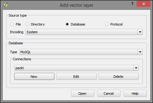
- Navigate to Layer | Add Layer | Add vector layer.
- Source type: Database
- Type: MySQL, as shown in the following screenshot:
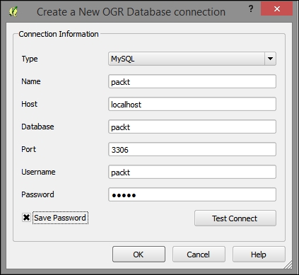
- Once you've indicated that you wish to add a MySQL Database layer, you will have the option to create a new connection. In Connections, click on New. In the dialog that opens, enter the following parameters, which we would have initially set up when we created our MySQL Database and imported the
.sqlbackup of thepacktschema:- Name:
packt - Host:
localhost - Database:
packt - Port:
3306 - Username:
packt - Password:
packt, as shown in the following screenshot:
- Name:
- Click on Test Connect.
- Click on OK.
- Click on Open, and the Select vector layers to add dialog will appear.
- From the Select vector layers dialog, click on Select All. This includes the following layers:
fieldsprecipitationrelative_humiditytemperature
- Click on OK.
The layers (actually just the data tables) from the MySQL Database will now appear in the QGIS Layers panel of your project.
The fields layer (table) is only one of the four tables we added to our project with latitude and longitude fields. We want this table to be recognized by QGIS as geospatial data and these coordinate pairs to be plotted in QGIS. Perform the following steps:
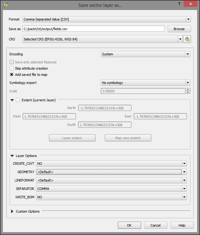
- Export the fields layer as CSV by right–clicking on the layer under the Layers panel and then clicking on Save as.
- In the Save vector layer as… dialog, perform the following steps:
- Click on Browse to choose a filesystem path to store the new
.csvfile. This file is included in the data underc6/data/output/fields.csv. - For GEOMETRY, select <Default>.
- All the other default fields can remain as they are given.
- Click on OK to save the new CSV, as shown in the following screenshot:
- Click on Browse to choose a filesystem path to store the new
Now, to import the CSV with the coordinate fields that are recognized as geospatial data and to plot the locations, perform the following steps:
- From the Layer menu, navigate to Add Layer | Add Delimited Text Layer.
- In Create a Layer from the Delimited Text File dialog, perform the following steps:
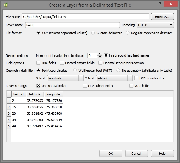
You will receive a notification that as no coordinate system was detected in this file, WGS 1984 was assigned. This is the correct coordinate system in our case, so no further intervention is necessary. After you dismiss this message, you will see the fields locations plotted on your map. If you don't, right–click on the new layer and select Zoom to Layer.
Note that this new layer is not reflected in a new file on the filesystem but is only stored with this QGIS project. This would be a good time to save your project.
Finally, join the other the other tables (precipitation, relative_humidity, and temperature) to the new plotted layer (fields) using the field_id field from each table one at a time. For a refresher on how to do this, refer to the Table join section of Chapter 1, Exploring Places – from Concept to Interface. To export each layer as separate shapefiles, right-click on each (precipitation, relative_humidity, and temperature), click on Save as, populate the path on which you want to save, and then save them.
The newer versions of QGIS support layer/table relations, which would allow us to model the one-to-many relationship between our locations, and an abstract measurement class that would include all the parameters. However, the use of table relationships is limited to a preliminary exploration of the relationships between layer objects and tables. The layer/table relationships are not recognized by any processing functions. Perform the following steps to explore the many-to-many layer/table relationships:
- Add a relation by navigating to Project | Project Properties | Relations. The following image is what you will see once the relationships to the three tables are established:
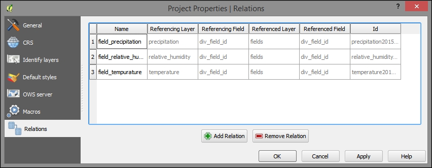
- To add a relation, select a nonlayer table (for example, precipitation) in the Referencing Layer (Child) field and a location table (for example, fields) in the Referenced Layer (Parent) field. Use the common Id field (for example,
field_id), which references the layer, to relate the tables. The name field can be filled arbitrarily, as shown in the following screenshot: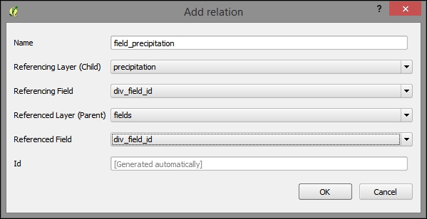
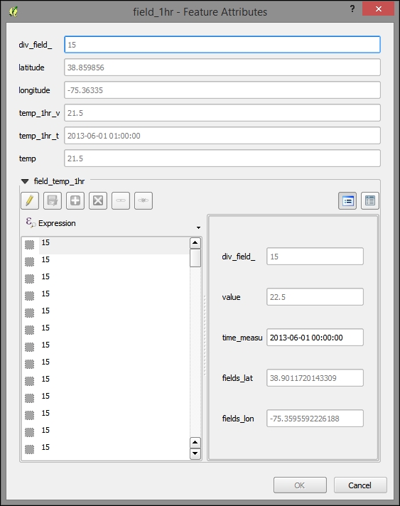
- Now, to use the relation, click on a geographic object in the parent layer using the identify tool (you need to check Auto open form in the identify tool options panel). You'll see all the child entities (rows) connected to this object.
Network Common Data Form (NetCDF) is a standard—and powerful—format for environmental data, such as meteorological data. NetCDF's strong suit is holding multidimensional data. With its abstract concept of dimension, NetCDF can handle the dimensions of latitude, longitude, and time in the same way that it handles other often physical, continuous, and ordinal data scales, such as air pressure levels.
For this project, we used the monthly global gridded high-resolution station (land) data for air temperature and precipitation from 1901-2010, which the NetCDF University of Delaware maintains as part of a collaboration with NOAA. You can download further data from this source at http://www.esrl.noaa.gov/psd/data/gridded/data.UDel_AirT_Precip.html.
While there is a plugin available, NetCDF can be viewed directly in QGIS, in GDAL via the command line, and in the QGIS Python Console. Perform the following steps:
- Navigate to Layer | Add Raster Layer.
- Browse to
c6/data/original/air.mon.mean.v301.ncand add this layer. - Use the path Raster | Miscellaneous > Information to find the range of the values in a band. In the initial dialog, click on OK to go to the information dialog and then look for
air_valid_range. You can see this information highlighted in the following image. Although QGIS's classifier will calculate the range for you, it is often thrown off by a numeric nodata value, which will typically skew the range to the lower end.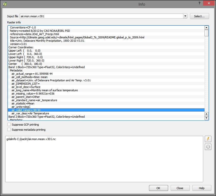
- Enter the range information (-90 to 50) into the Style tab of the Layer Properties tab.
- Click on Invert to show cool to hot colors from less to more, just as you would expect with temperature.
- Click on Classify to create the new bins based on the number and color range. The following screenshot shows what an ideal selection of bins and colors would look like:
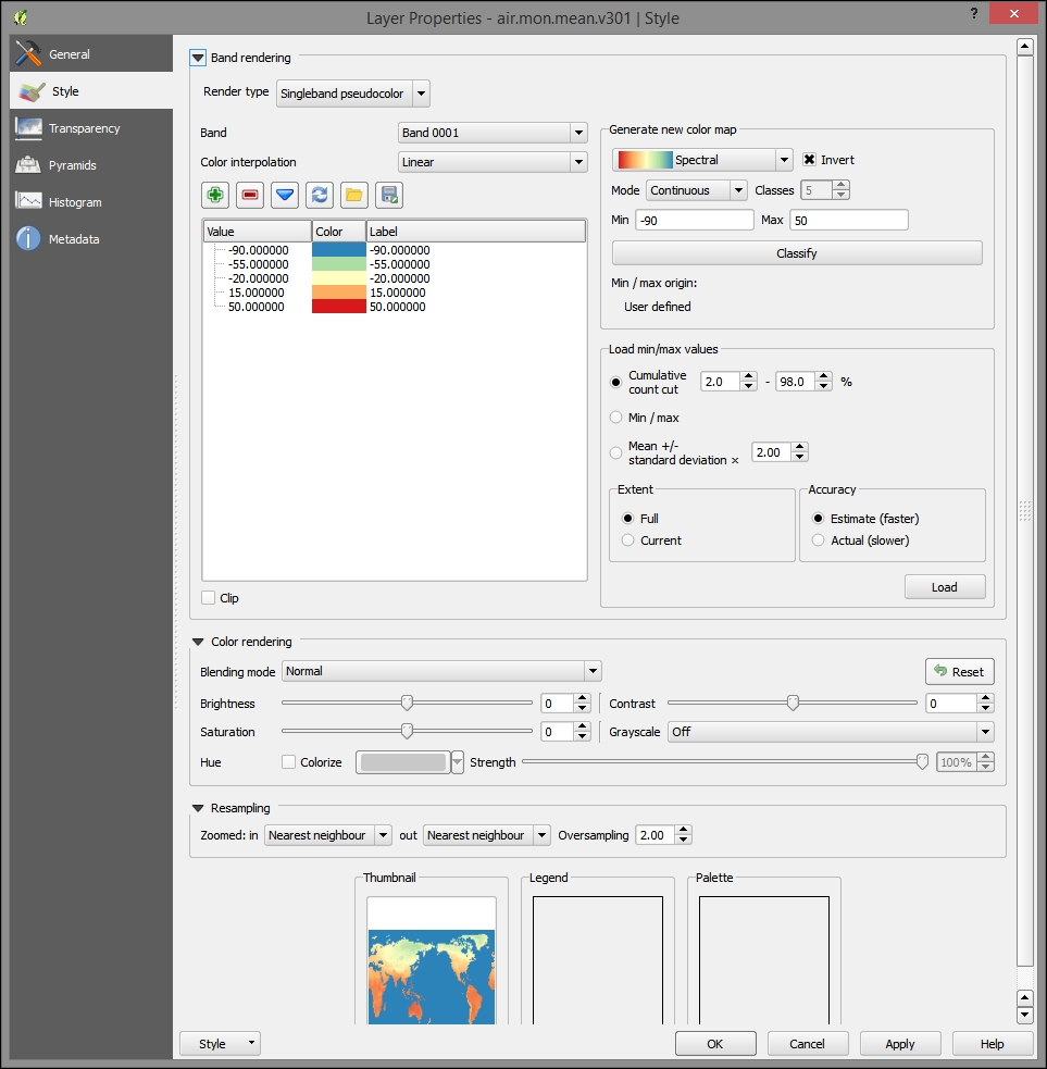
- Click on OK. The end result will look similar to the following image:
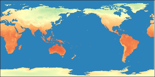
To render the gridded NetCDF data accessible to certain models, databases, and to web interaction, you could write a workflow program similar to the following after sampling the gridded values and attaching them to the points for each time period.