Acquiring data for geospatial applications

After any preliminary planning—a step that should include careful consideration of at least the use cases for our application—we must acquire data. Acquisition involves not only the physical transfer of the data, but also processing the data to a particular format and importing it into whatever data storage scheme we have developed. This is usually called Extract, Transform, and Load (ETL).

Though ETL is the first major step in developing a web application, it should not be taken lightly. As with any information-based project, data often comes to us in a form that's not immediately useable—whether because of nonuniform formatting, uncertain metadata, or unknown field mapping. Although any of these can affect a GIS project, as GISs are organized around cartographic coordinate systems, the principle concern is usually that data must be spatially described in a uniform way, namely by a single CRS, as referred to earlier. To that end, data often requires georeferencing and spatial reference manipulation.

For certain datasets, an ETL workflow is unnecessary because the data is already provided via web services. Using hosted data stored on the remote server and read directly from the Web by your application is a very attractive option, purely for ease of development if nothing else. However, you'll probably need to change the CRS, and possibly other formatting, of your local data to match that of the hosted data since hosted services are rarely provided in multiple CRSs. You must also consider whether the hosted data provides capabilities that support the interface of your application. You will find more information on this topic under the operational layer section of this chapter.

Producing geospatial data with georeferencing

By georeferencing, or attaching our data to coordinates, we assert the geographic location of each object in our data. Once our data is georeferenced, we can call it geospatial. Georeferencing is done according to the fields in the data and those available in some geospatial reference source.

The simplest example is when a data field actually matches a field in some existing geospatial data. This data field is often an ID number or name. This kind of georeferencing is called a table join.

Table join

In this example, we will take a look at a table join with some temperature data from an unknown source and census tract boundaries from the US Census. Census' TIGER/Line files are generally the first places to look for U.S. national boundary files of all sorts, not just census tabulation areas.

The temperature data to be georeferenced through a table join would be as follows:

tract,date,mean_temp
014501,2010-06-01,73
014402,2010-06-01,75
014703,2010-06-01,75
014100,2010-06-01,76
014502,2010-06-01,75
014403,2010-06-01,75
014300,2010-06-01,71
014200,2010-06-01,72
013610,2010-06-01,68

Temperature data metadata would be as follows:

"String","Date","Integer"

Tip

Downloading the example code

You can download the example code files for all Packt books you have purchased from your account at http://www.packtpub.com. If you purchased this book elsewhere, you can visit http://www.packtpub.com/support and register to have the files e-mailed directly to you.

To perform a table join, perform the following steps:

Copy the code from the first information box calls into a text file and save this as temperature.csv.
Tip
The CSVT format is a metadata file that accompanies a CSV file of the same name. It defines column data types.
Copy the code from the second information box into a text file and save this as temperature.csvt. Otherwise, QGIS will not know what type of data is contained in each column.
Tip
Data for all the chapters will be found under the data directory for each chapter. You can use the included data under c1/data/original with the file names given earlier. Besides selecting the browse menu, you can also just drag the file into the Layers panel from an open operating system window. You can find examples of data output during exercises under the output directory of each chapter's data directory. This is also the directory given in the instructions as the destination directory for your output. You will probably want to create a new directory for your output and save your data there so as to not overwrite the included reference data.
Navigate to Layer | Add Layer | Add Vector Layer | Browse to, and select temperature.csv.
Tip
CSV data can also be added through Layer | Add Layer | Add Delimited Text. This is especially useful to plot coordinates in a CSV, as you'll see later.
Download the Tract boundary data:
1. Visit http://www.census.gov/geo/maps-data/data/tiger-line.html.
2. Click on the tab for the year you wish to find.
3. Download the web interface.
4. This will take us to http://www.census.gov/cgi-bin/geo/shapefiles2014/main.
5. Navigate to Layer Type | Census Tracts and click on the submit button. Now, select Delaware from the Census Tract (2010) dropdown. Click on Submit again. Now select All counties in one state-based file from the dropdown displayed on this page and finally click on Download.
6. Unzip the downloaded folder.
Navigate to Layer | Add Layer | Add Vector Layer | Browse to, and select the tl_2010_10_tract10.shp file in the unzipped directory.
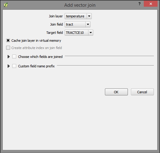
Right-click on tl_2010_10_tract10 in the Layer panel, and then navigate to Properties | Joins. Click on the button with the green plus sign (+) to add a join.
Select temperature as the Join layer option, tract as the Join field option, TRACTCE10 as the Target field option, and click on OK on this and the properties dialog:

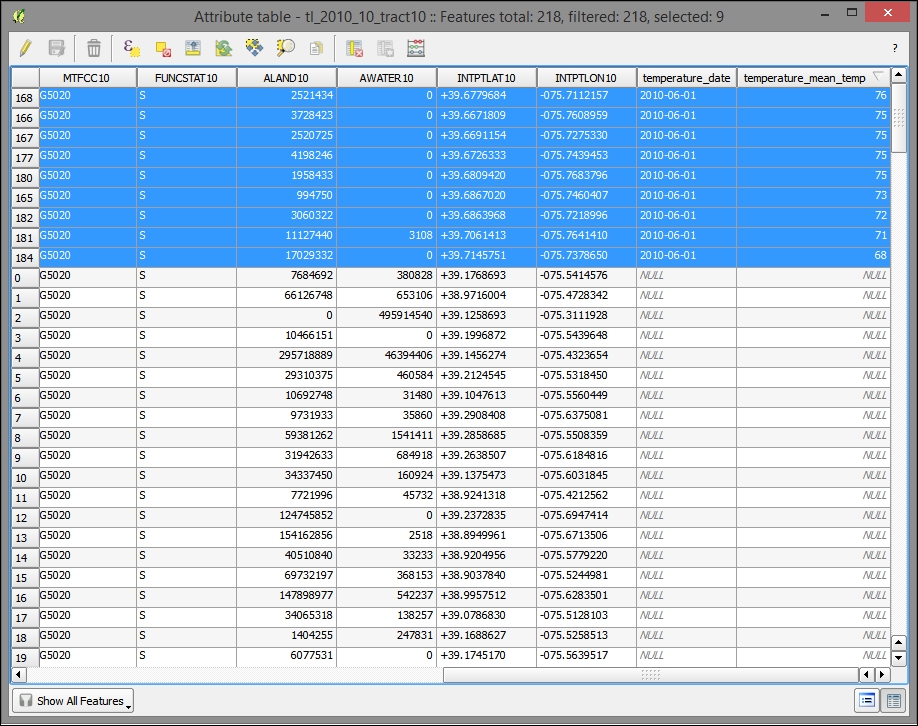
To verify that the join completed, open the attribute table of the target layer (such as the geospatial reference, in this case, tl_2010_10) and sort by the new temperature_mean_temp field. Notice that the fields and values from the join layer are now included in the target layer.

Select the target layer, tl_2010_10_tract10, from the Layers panel.
Navigate to Layer | Open attribute table.
Click on the temperature_mean_temp column header to sort tracts by this column. You may have to click twice to toggle the sort order from ascending to descending.

Geocode

If our data is expressed as addresses, intersections, or other well-known places, we can geocode it (that is, match it with coordinates) with a local or remote geocoder configured for our particular set of fields, such as the standard fields in an address.

In this example, we will geocode it using the remote geocoder provided by Google. Perform the following steps:

Install the MMQGIS plugin.
If you don't already have some address data to work with, you can make up a delimited file that contains some standard address fields, such as street, city, state, and county (ZIP code is not used by this plugin). The data that I'm using comes from New Castle County, Delaware's GIS site (http://gis.nccde.org/gis_viewer/).
Whether you've downloaded your address data or made up your own, make sure to create a header row. Otherwise, MMQGIS fails to geocode.
The following is an example of MMQGIS-friendly address data:
```
id,address,city,state,zip,country
1801300170,44 W CLEVELAND AV,NEWARK,DE,19711,USA
1801400004,85 N COLLEGE AV,NEWARK,DE,19711,USA
1802600068,501 ACADEMY ST,NEWARK,DE,19716,USA
```
Open the MMQGIS geocode dialog by navigating to MMQGIS | Geocode | Geocode CSV with Google/OpenStreetMap.
Once you've matched your fields to the address input fields available, you have the option of choosing Google Maps or OpenStreetMap. Google Maps usually have a much higher rate of success, while OpenStreetMap has the value of not having a daily limit on the number of addresses you can geocode. At this time, the OSM geocoder produces such poor results as to not be useful.
You'll want to manually select or input a filesystem path for a notfound.csv file for the final input. The default file location can be problematic.
Once your geocode is complete, you'll see how well the geocode address text matched with our geocoder reference. You may wish to alter addresses in the notfound.csv file and attempt to geocode these again.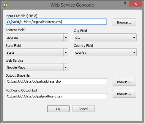

Orthorectify

Finally, if our data is an image or grid (raster), we can match up locations in the image with known locations in a reference map. The registration of these pairs and subsequent transformation of the grid is called orthorectification or sometimes by the more generic term, georeferencing (even though that applies to a wider range of operations).

Add a basemap, to be used for reference:
1. Add the OpenLayers plugin. Navigate to Plugins | Manage | Install Plugins; select OpenLayers Plugin and click on Install.
2. Navigate to Web | OpenLayers plugin, and select the basemap of your choice. MapQuest-OSM is a good option.
Obtain map image:
1. I have downloaded a high-resolution image (c1/data/original/4622009.jpg) from David Rumsey Map Collection, MapRank Search (http://rumsey.mapranksearch.com/), which is an excellent source for historical map images of the United States.
2. Search by a location, filtering by time, scale, and other attributes. You can find the image we use by searching for Newark, Delaware.
3. Once you find your map, navigate to it. Then, find Export in the upper right-hand corner, and export an extra high-resolution image.
4. Unzip the downloaded folder.
Orthorectify/georeference the image with the following steps:
1. Install and enable the Georeferencer GDAL plugin.
2. Navigate to Raster | Georeferencer | Georeferencer.
3. Pan and zoom the reference basemap in the canvas on a location that you recognize in the map image.
4. Pan and zoom on the map image.
5. Select Add Control Point if it is not already selected.
6. Click on the location in the map image that you recognized in the third step.
7. Click the Pencil icon to choose control point from Map Canvas.
8. Click on the location in the reference basemap.
9. Click on OK.
10. Add three of these control points, as shown in the following screenshot:
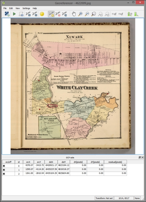
11. Start georeferencing by clicking on the Play button.
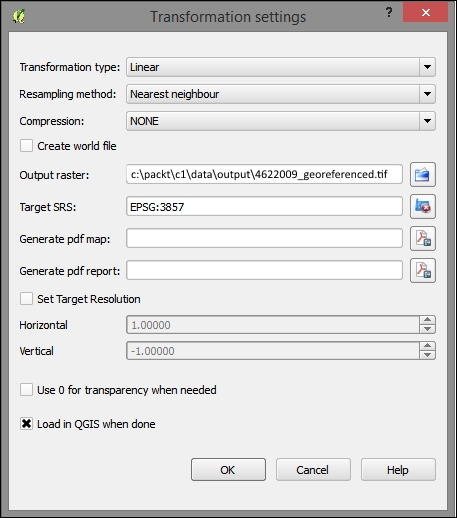
12. Enter the transformation settings information, as shown in the following screenshot:
Now, start georeferencing by clicking on the Play button again.

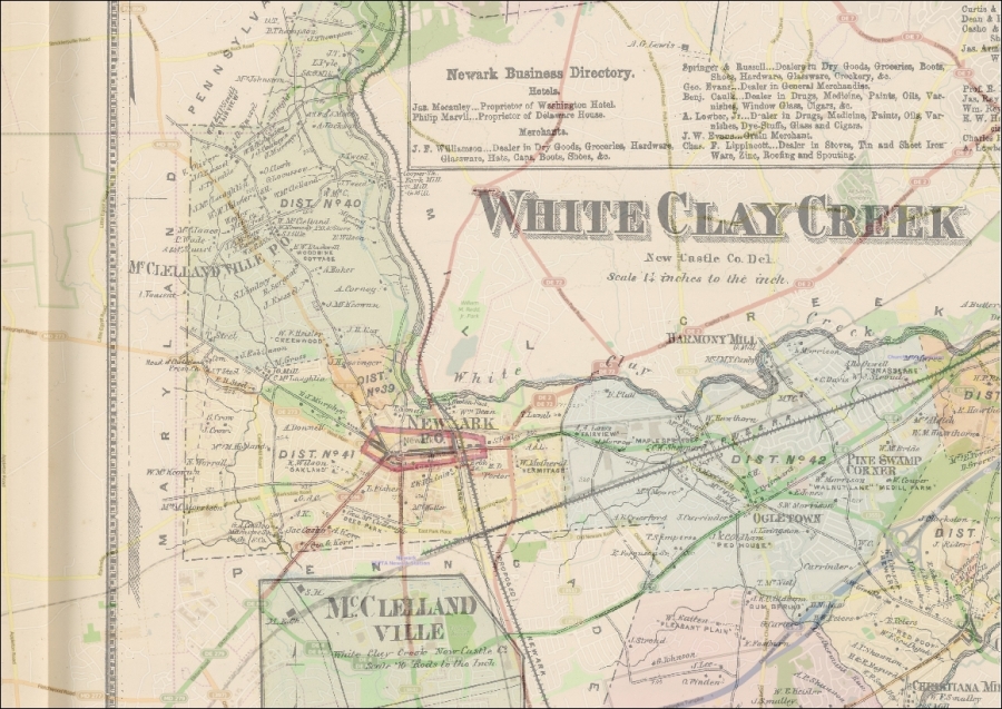
Once your image has been georeferenced, you should see it align with the other data on your map. You can alter the layer transparency under Layer properties | Transparency:

The spatial reference manipulation – making the coordinates line up

QGIS will sometimes do an On-the-Fly (OTF) projection of all the data added to the canvas on the project CRS (defined under Project | Project Properties | CRS). You will want to disable OTF projection in the projects you intend to produce for web applications, as all layers should have their own spatial reference independently defined and transformed or projected in the same CRS, if needed.

Setting CRS

When geospatial data is received with no metadata on what the spatial reference system describes its coordinates, it is necessary to assign a system. This can be by right-clicking on the layer in Layers Panel | Save as and selecting the new CRS.

Transformation and projection

At other times, data is received with a different CRS than in the case of the other data used in the project. When CRSs differ, care should be taken to see whether to alter the CRS of the new nonconforming data or of the existing data. Of course we want to choose a system that supports our needs for accuracy or extent; at other times when we already have a suitable basemap, we will want operational layers to conform to the basemap's system. When a suitable basemap is already available to be consumed by our web application, we can often use the system of the basemap for the project. All major third-party basemap providers use Web Mercator, which is now known as EPSG:3857.

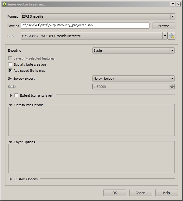
You can project data from geographic to projected coordinates or from one projection to another. This can be done in the same way as you would define a projection: by right-clicking on a layer in Layers Panel | Save as and selecting the new CRS. An appropriate transformation will generally be applied by default.

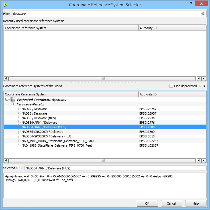
There are some features in CRS Selector that you should be aware of. By selecting from Recently used coordinate reference systems, you can often easily match up a new CRS with those existing in the workspace. You also have the option to search through the available systems by entering the Filter input. You will see the PROJ.4 WKT representation of the selected CRS at the bottom of the dialog.

Previous Chapter

1. Exploring Places – from Concept to Interface

Next Chapter

Visualizing GIS data