You'll need a raster that lacks spatial reference information; that is, unknown projection according to QGIS. You'll also need a second layer (reference map) that is known and you can use for reference points. The exception to this is, if you have a paper map that has coordinates marked on it or a spatial dataset that just didn't come with a reference file but you happen to know its CRS/SRS definition. Load your reference map in QGIS.

This book's data includes a scanned USGS topographic map that's missing its o38121e7.tif projection information. This map is from Davis, CA, so the example data has plenty of other possible reference layers you could use, for example, the streets would be a good choice.

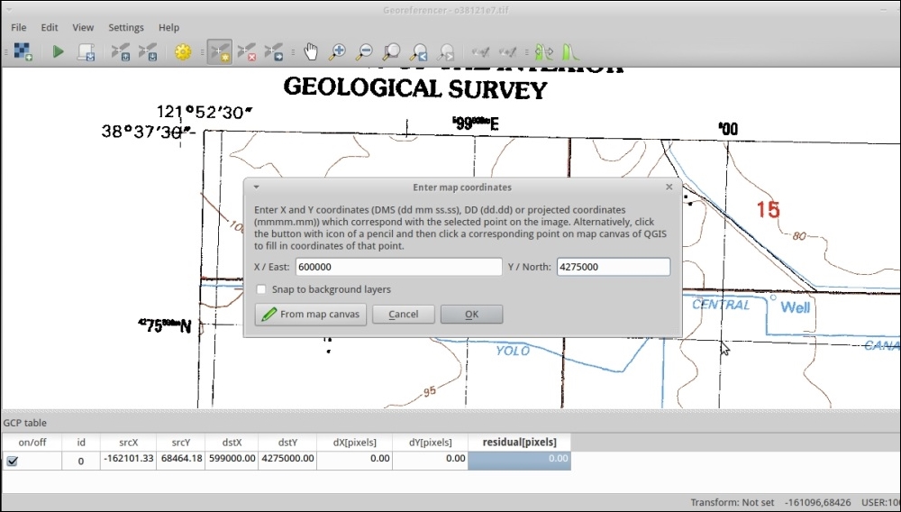
On the Raster menu, open the Georeferencing tool and perform the following steps:

A mathematical function is created based on the differences between your two sets of points. This function is then applied to the whole image, stretching it in an attempt to fit. This is basically a translation or projection from one coordinate system to another.

Picking transformation types can be a little tricky, the list in QGIS is currently in alphabetical order and not the recommended order. Polynomial 2 and Thin-plate-spline (TPS) are probably the two most common choices. Polynomial 1 is great when you just have minor shift, zooming (scale), and rotation. When you have old well-made maps in consistent projections, this will apply the least amount of change. Polynomial 2 picks up from here and handles consistent distortion. Both of these provide you with an error estimate as the Residual or RMSE (Root Mean Square Error). TPS handles variable distortion, varying it's correction around each control point. This will almost always result in the best fit, at least through the GCPs that you provide. However, because it varies at every GCP location, you can't calculate an error estimate and it may actually overfit (create new distortion). TPS is best for hand-drawn maps, nonflat scans of maps, or other variable distorted sources. Polynomial methods are good for sources that had high accuracy and reference marks to begin with.

If you really want a good match, once you have all your points, check the RMSE values in the table at the bottom. Generally, you want this near or less than 1. If you have a point with a huge value, consider deleting it or redoing it. You can move existing points, and a line will be drawn in the direction of the estimated error. So, go back over the high values, zoom in extra close, and use the GCP move option.

Sometimes, just changing your transformation type will help, as shown in the following screenshot that compares Polynomial 1 versus Polynomial 2 for the same set of GCP:

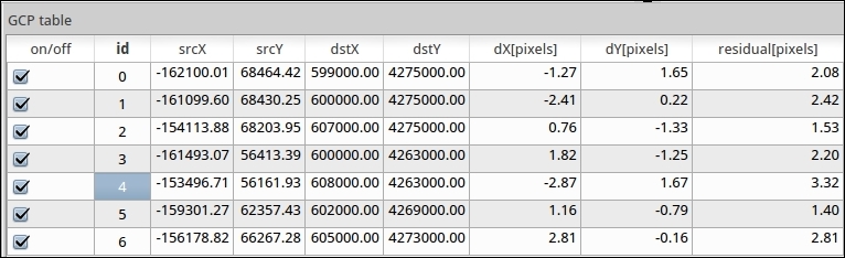
Polynomial 1

Note the residual values difference when changing to Polynomial 2 (assuming that you have the minimum number of points to use Polynomial 2):

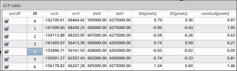
Polynomial 2