Table of Contents for
QGIS: Becoming a GIS Power User
 QGIS: Becoming a GIS Power User
Published by
Packt Publishing, 2017
QGIS: Becoming a GIS Power User
Published by
Packt Publishing, 2017
- Cover
- Table of Contents
- QGIS: Becoming a GIS Power User
- QGIS: Becoming a GIS Power User
- QGIS: Becoming a GIS Power User
- Credits
- Preface
- What you need for this learning path
- Who this learning path is for
- Reader feedback
- Customer support
- 1. Module 1
- 1. Getting Started with QGIS
- Running QGIS for the first time
- Introducing the QGIS user interface
- Finding help and reporting issues
- Summary
- 2. Viewing Spatial Data
- Dealing with coordinate reference systems
- Loading raster files
- Loading data from databases
- Loading data from OGC web services
- Styling raster layers
- Styling vector layers
- Loading background maps
- Dealing with project files
- Summary
- 3. Data Creation and Editing
- Working with feature selection tools
- Editing vector geometries
- Using measuring tools
- Editing attributes
- Reprojecting and converting vector and raster data
- Joining tabular data
- Using temporary scratch layers
- Checking for topological errors and fixing them
- Adding data to spatial databases
- Summary
- 4. Spatial Analysis
- Combining raster and vector data
- Vector and raster analysis with Processing
- Leveraging the power of spatial databases
- Summary
- 5. Creating Great Maps
- Labeling
- Designing print maps
- Presenting your maps online
- Summary
- 6. Extending QGIS with Python
- Getting to know the Python Console
- Creating custom geoprocessing scripts using Python
- Developing your first plugin
- Summary
- 2. Module 2
- 1. Exploring Places – from Concept to Interface
- Acquiring data for geospatial applications
- Visualizing GIS data
- The basemap
- Summary
- 2. Identifying the Best Places
- Raster analysis
- Publishing the results as a web application
- Summary
- 3. Discovering Physical Relationships
- Spatial join for a performant operational layer interaction
- The CartoDB platform
- Leaflet and an external API: CartoDB SQL
- Summary
- 4. Finding the Best Way to Get There
- OpenStreetMap data for topology
- Database importing and topological relationships
- Creating the travel time isochron polygons
- Generating the shortest paths for all students
- Web applications – creating safe corridors
- Summary
- 5. Demonstrating Change
- TopoJSON
- The D3 data visualization library
- Summary
- 6. Estimating Unknown Values
- Interpolated model values
- A dynamic web application – OpenLayers AJAX with Python and SpatiaLite
- Summary
- 7. Mapping for Enterprises and Communities
- The cartographic rendering of geospatial data – MBTiles and UTFGrid
- Interacting with Mapbox services
- Putting it all together
- Going further – local MBTiles hosting with TileStream
- Summary
- 3. Module 3
- 1. Data Input and Output
- Finding geospatial data on your computer
- Describing data sources
- Importing data from text files
- Importing KML/KMZ files
- Importing DXF/DWG files
- Opening a NetCDF file
- Saving a vector layer
- Saving a raster layer
- Reprojecting a layer
- Batch format conversion
- Batch reprojection
- Loading vector layers into SpatiaLite
- Loading vector layers into PostGIS
- 2. Data Management
- Joining layer data
- Cleaning up the attribute table
- Configuring relations
- Joining tables in databases
- Creating views in SpatiaLite
- Creating views in PostGIS
- Creating spatial indexes
- Georeferencing rasters
- Georeferencing vector layers
- Creating raster overviews (pyramids)
- Building virtual rasters (catalogs)
- 3. Common Data Preprocessing Steps
- Converting points to lines to polygons and back – QGIS
- Converting points to lines to polygons and back – SpatiaLite
- Converting points to lines to polygons and back – PostGIS
- Cropping rasters
- Clipping vectors
- Extracting vectors
- Converting rasters to vectors
- Converting vectors to rasters
- Building DateTime strings
- Geotagging photos
- 4. Data Exploration
- Listing unique values in a column
- Exploring numeric value distribution in a column
- Exploring spatiotemporal vector data using Time Manager
- Creating animations using Time Manager
- Designing time-dependent styles
- Loading BaseMaps with the QuickMapServices plugin
- Loading BaseMaps with the OpenLayers plugin
- Viewing geotagged photos
- 5. Classic Vector Analysis
- Selecting optimum sites
- Dasymetric mapping
- Calculating regional statistics
- Estimating density heatmaps
- Estimating values based on samples
- 6. Network Analysis
- Creating a simple routing network
- Calculating the shortest paths using the Road graph plugin
- Routing with one-way streets in the Road graph plugin
- Calculating the shortest paths with the QGIS network analysis library
- Routing point sequences
- Automating multiple route computation using batch processing
- Matching points to the nearest line
- Creating a routing network for pgRouting
- Visualizing the pgRouting results in QGIS
- Using the pgRoutingLayer plugin for convenience
- Getting network data from the OSM
- 7. Raster Analysis I
- Using the raster calculator
- Preparing elevation data
- Calculating a slope
- Calculating a hillshade layer
- Analyzing hydrology
- Calculating a topographic index
- Automating analysis tasks using the graphical modeler
- 8. Raster Analysis II
- Calculating NDVI
- Handling null values
- Setting extents with masks
- Sampling a raster layer
- Visualizing multispectral layers
- Modifying and reclassifying values in raster layers
- Performing supervised classification of raster layers
- 9. QGIS and the Web
- Using web services
- Using WFS and WFS-T
- Searching CSW
- Using WMS and WMS Tiles
- Using WCS
- Using GDAL
- Serving web maps with the QGIS server
- Scale-dependent rendering
- Hooking up web clients
- Managing GeoServer from QGIS
- 10. Cartography Tips
- Using Rule Based Rendering
- Handling transparencies
- Understanding the feature and layer blending modes
- Saving and loading styles
- Configuring data-defined labels
- Creating custom SVG graphics
- Making pretty graticules in any projection
- Making useful graticules in printed maps
- Creating a map series using Atlas
- 11. Extending QGIS
- Defining custom projections
- Working near the dateline
- Working offline
- Using the QspatiaLite plugin
- Adding plugins with Python dependencies
- Using the Python console
- Writing Processing algorithms
- Writing QGIS plugins
- Using external tools
- 12. Up and Coming
- Preparing LiDAR data
- Opening File Geodatabases with the OpenFileGDB driver
- Using Geopackages
- The PostGIS Topology Editor plugin
- The Topology Checker plugin
- GRASS Topology tools
- Hunting for bugs
- Reporting bugs
- Bibliography
- Index
In this recipe, we will look at the different layer and feature blending modes. Using these tools, we can achieve special rendering effects, which you may already know from other graphics programs.
To follow this recipe, you just need to load stamen.png and effect.png from our sample data. Make sure that stamen (left-hand side in the following screenshot) is the lower layer and effect (right-hand side in the following screenshot) is the upper layer. To test the feature blending modes, load blending.shp:
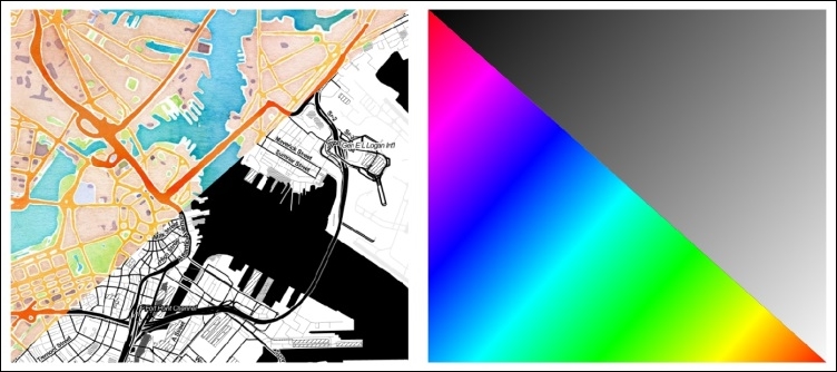
(Background maps "Watercolor" and "Toner" by Stamen Design, under CC BY 3.0. Data by OpenStreetMap, under CC BY SA).
Using the two raster layers, we can try the different blending modes. Of course, this works for vector layers, as well:
- Double-click on the
effectslayer to open Layer Properties. - You can find the blending settings by going to Layer Properties | Style | Color Rending together with other helpful controls for Brightness, Contrast, Saturation, and more, as shown in the next screenshot:
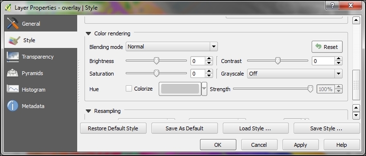
- Change the Blending mode and click on Apply to see the results.
- Similarly, for vector layers, such as our blending layer, we find the blending mode settings by going to Layer Properties | Style | Layer rendering, as shown in the following screenshot:
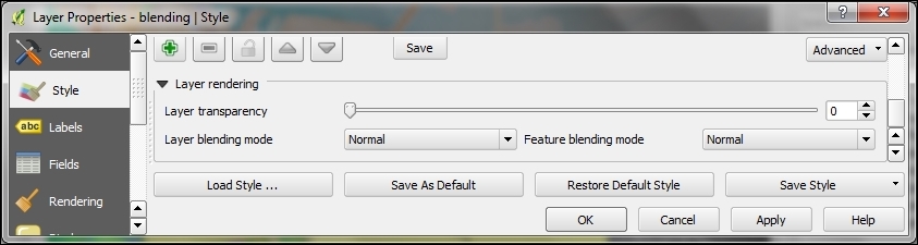
The main difference is that, for vector layers, we can control how features are blended together, and how the result is then blended to the underlying layers using the Feature blending and Layer blending modes, respectively. The feature blending mode is applied on a per-feature-basis.
The following screenshot shows the differences between feature and layer blending:
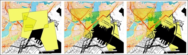
Feature and/or layer blending in action (from left to right): feature blending only, layer blending only, feature and layer blending combined (background maps "Watercolor" and "Toner" by Stamen Design, under CC BY 3.0. Data by OpenStreetMap, under CC BY SA).
The following is an explanation of the preceding screenshots:
- The leftmost image shows that Feature blending mode is set to Multiply, while Layer blending mode is set to default, Normal. This results in a map where the vector features are rendered on top of each other using the Multiply mode before the whole layer is overlaid on top of the lower layer(s).
- The center image instead shows Normal Feature blending mode combined with Multiply Layer blending mode. You can see how the features can block each other out because they are drawn on top of each other.
- Finally, the rightmost image shows both Layer blending mode and Feature blending modes being set to Multiply. In this combination, the Multiply rule is applied on both the feature and the layer level and, therefore, we can see features and the underlying background layer(s) shining through the features in the upper layer.
Based on the selected blending mode, the pixel colors (in the RGB mode) of the lower and upper layers are mixed as described next. For illustration and quick reference, the following figure shows the results of all 12 blending modes (from left to right and top to bottom), except for the Normal setting, which does not mix the colors but only uses the alpha channel of the upper layer to blend with the layer below it:
- Lighten: The Lighten mode selects the maximum of each RGB component from the foreground and background pixels. Be aware that the results tend to be jagged and harsh.
- Screen: The Screen mode paints light pixels from the upper layer over the lower layer, but it skips the dark pixels.
- Dodge: The Dodge mode will brighten and saturate the lower layer based on the lightness of the upper layer. This means that brighter colors in the upper layer cause the saturation and brightness of the lower layer to increase. This works best if the top pixels aren't too bright; otherwise, the effect is quite extreme.
- Addition: The Addition mode adds the pixel values of both layers. If the result exceeds 1 (in the case of RGB), the respective areas are displayed in white.
- Darken: The Darken mode creates a result that retains the smallest RGB components of both layers. Therefore, this is the opposite of the Lighten mode and, just as with Lighten, the results tend to be jagged and harsh.
- Multiply: The Multiply mode multiplies the values of both layers, thus resulting in a darker picture.
- Burn: The Burn mode causes darker colors in the upper layer to darken the lower layer. Burn can be used to tweak and colorize underlying layers.
- Overlay: The Overlay mode combines the Multiply and Screen blending modes. As a result, light parts become lighter and dark parts become darker.
- Soft light: The Soft light mode is very similar to Overlay, but it uses a combination of Burn and Dodge. This is supposed to emulate shining a soft light on an image.
- Hard light: The Hard light mode is also very similar to Overlay. It is supposed to emulate projecting a very intense light on an image.
- Difference: The Difference mode subtracts the values of the upper layer from the lower layer (or the other way around) to always get a positive value. Blending with black (which has an RGB value of 0,0,0) produces no change.
- Subtract: The Subtract mode subtracts the values of one layer from the other. In the case of negative values, black is displayed:
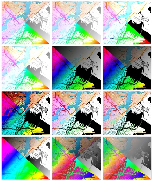
Overview of the 12 blending modes (background maps "Watercolor" and "Toner" by Stamen Design, under CC BY 3.0. Data by OpenStreetMap, under CC BY SA): first row: Lighten, Screen, and Dodge; second row: Addition, Darken, and Multiply; third row: Burn, Overlay, and Soft light; fourth row: Hard light, Difference, and Subtract.