Table of Contents for
QGIS: Becoming a GIS Power User
 QGIS: Becoming a GIS Power User
Published by
Packt Publishing, 2017
QGIS: Becoming a GIS Power User
Published by
Packt Publishing, 2017
- Cover
- Table of Contents
- QGIS: Becoming a GIS Power User
- QGIS: Becoming a GIS Power User
- QGIS: Becoming a GIS Power User
- Credits
- Preface
- What you need for this learning path
- Who this learning path is for
- Reader feedback
- Customer support
- 1. Module 1
- 1. Getting Started with QGIS
- Running QGIS for the first time
- Introducing the QGIS user interface
- Finding help and reporting issues
- Summary
- 2. Viewing Spatial Data
- Dealing with coordinate reference systems
- Loading raster files
- Loading data from databases
- Loading data from OGC web services
- Styling raster layers
- Styling vector layers
- Loading background maps
- Dealing with project files
- Summary
- 3. Data Creation and Editing
- Working with feature selection tools
- Editing vector geometries
- Using measuring tools
- Editing attributes
- Reprojecting and converting vector and raster data
- Joining tabular data
- Using temporary scratch layers
- Checking for topological errors and fixing them
- Adding data to spatial databases
- Summary
- 4. Spatial Analysis
- Combining raster and vector data
- Vector and raster analysis with Processing
- Leveraging the power of spatial databases
- Summary
- 5. Creating Great Maps
- Labeling
- Designing print maps
- Presenting your maps online
- Summary
- 6. Extending QGIS with Python
- Getting to know the Python Console
- Creating custom geoprocessing scripts using Python
- Developing your first plugin
- Summary
- 2. Module 2
- 1. Exploring Places – from Concept to Interface
- Acquiring data for geospatial applications
- Visualizing GIS data
- The basemap
- Summary
- 2. Identifying the Best Places
- Raster analysis
- Publishing the results as a web application
- Summary
- 3. Discovering Physical Relationships
- Spatial join for a performant operational layer interaction
- The CartoDB platform
- Leaflet and an external API: CartoDB SQL
- Summary
- 4. Finding the Best Way to Get There
- OpenStreetMap data for topology
- Database importing and topological relationships
- Creating the travel time isochron polygons
- Generating the shortest paths for all students
- Web applications – creating safe corridors
- Summary
- 5. Demonstrating Change
- TopoJSON
- The D3 data visualization library
- Summary
- 6. Estimating Unknown Values
- Interpolated model values
- A dynamic web application – OpenLayers AJAX with Python and SpatiaLite
- Summary
- 7. Mapping for Enterprises and Communities
- The cartographic rendering of geospatial data – MBTiles and UTFGrid
- Interacting with Mapbox services
- Putting it all together
- Going further – local MBTiles hosting with TileStream
- Summary
- 3. Module 3
- 1. Data Input and Output
- Finding geospatial data on your computer
- Describing data sources
- Importing data from text files
- Importing KML/KMZ files
- Importing DXF/DWG files
- Opening a NetCDF file
- Saving a vector layer
- Saving a raster layer
- Reprojecting a layer
- Batch format conversion
- Batch reprojection
- Loading vector layers into SpatiaLite
- Loading vector layers into PostGIS
- 2. Data Management
- Joining layer data
- Cleaning up the attribute table
- Configuring relations
- Joining tables in databases
- Creating views in SpatiaLite
- Creating views in PostGIS
- Creating spatial indexes
- Georeferencing rasters
- Georeferencing vector layers
- Creating raster overviews (pyramids)
- Building virtual rasters (catalogs)
- 3. Common Data Preprocessing Steps
- Converting points to lines to polygons and back – QGIS
- Converting points to lines to polygons and back – SpatiaLite
- Converting points to lines to polygons and back – PostGIS
- Cropping rasters
- Clipping vectors
- Extracting vectors
- Converting rasters to vectors
- Converting vectors to rasters
- Building DateTime strings
- Geotagging photos
- 4. Data Exploration
- Listing unique values in a column
- Exploring numeric value distribution in a column
- Exploring spatiotemporal vector data using Time Manager
- Creating animations using Time Manager
- Designing time-dependent styles
- Loading BaseMaps with the QuickMapServices plugin
- Loading BaseMaps with the OpenLayers plugin
- Viewing geotagged photos
- 5. Classic Vector Analysis
- Selecting optimum sites
- Dasymetric mapping
- Calculating regional statistics
- Estimating density heatmaps
- Estimating values based on samples
- 6. Network Analysis
- Creating a simple routing network
- Calculating the shortest paths using the Road graph plugin
- Routing with one-way streets in the Road graph plugin
- Calculating the shortest paths with the QGIS network analysis library
- Routing point sequences
- Automating multiple route computation using batch processing
- Matching points to the nearest line
- Creating a routing network for pgRouting
- Visualizing the pgRouting results in QGIS
- Using the pgRoutingLayer plugin for convenience
- Getting network data from the OSM
- 7. Raster Analysis I
- Using the raster calculator
- Preparing elevation data
- Calculating a slope
- Calculating a hillshade layer
- Analyzing hydrology
- Calculating a topographic index
- Automating analysis tasks using the graphical modeler
- 8. Raster Analysis II
- Calculating NDVI
- Handling null values
- Setting extents with masks
- Sampling a raster layer
- Visualizing multispectral layers
- Modifying and reclassifying values in raster layers
- Performing supervised classification of raster layers
- 9. QGIS and the Web
- Using web services
- Using WFS and WFS-T
- Searching CSW
- Using WMS and WMS Tiles
- Using WCS
- Using GDAL
- Serving web maps with the QGIS server
- Scale-dependent rendering
- Hooking up web clients
- Managing GeoServer from QGIS
- 10. Cartography Tips
- Using Rule Based Rendering
- Handling transparencies
- Understanding the feature and layer blending modes
- Saving and loading styles
- Configuring data-defined labels
- Creating custom SVG graphics
- Making pretty graticules in any projection
- Making useful graticules in printed maps
- Creating a map series using Atlas
- 11. Extending QGIS
- Defining custom projections
- Working near the dateline
- Working offline
- Using the QspatiaLite plugin
- Adding plugins with Python dependencies
- Using the Python console
- Writing Processing algorithms
- Writing QGIS plugins
- Using external tools
- 12. Up and Coming
- Preparing LiDAR data
- Opening File Geodatabases with the OpenFileGDB driver
- Using Geopackages
- The PostGIS Topology Editor plugin
- The Topology Checker plugin
- GRASS Topology tools
- Hunting for bugs
- Reporting bugs
- Bibliography
- Index
In Chapter 4, Spatial Analysis, we used the tools of Processing Toolbox to analyze our data, but we are not limited to these tools. We can expand processing with our own scripts. The advantages of processing scripts over normal Python scripts, such as the ones we saw in the previous section, are as follows:
- Processing automatically generates a graphical user interface for the script to configure the script parameters
- Processing scripts can be used in Graphical modeler to create geoprocessing models
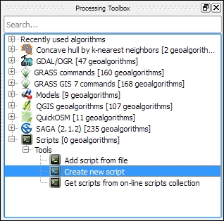
As the following screenshot shows, the Scripts section is initially empty, except for some Tools to add and create new scripts:
We will create our first simple script; which fetches some layer information. To get started, double-click on the Create new script entry in Scripts | Tools. This opens an empty Script editor dialog. The following screenshot shows the Script editor with a short script that prints the input layer's name on the Python Console:
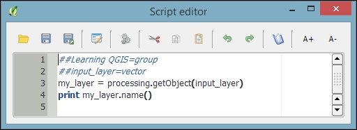
The first line means our script will be put into the Learning QGIS group of scripts, as shown in the following screenshot. The double hashes (##) are Processing syntax and they indicate that the line contains Processing-specific information rather than Python code. The script name is created from the filename you chose when you saved the script. For this example, I have saved the script as my_first_script.py. The second line defines the script input, a vector layer in this case. On the following line, we use Processing's getObject() function to get access to the input layer object, and finally the layer name is printed on the Python Console.
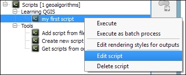
You can run the script either directly from within the editor by clicking on the Run algorithm button, or by double-clicking on the entry in the Processing Toolbox. If you want to change the code, use Edit script from the entry context menu, as shown in this screenshot:
Tip
A good way of learning how to write custom scripts for Processing is to take a look at existing scripts, for example, at https://github.com/qgis/QGIS-Processing/tree/master/scripts. This is the official script repository, where you can also download scripts using the built-in Get scripts from on-line scripts collection tool in the Processing Toolbox.
Of course, in most cases, we don't want to just output something on the Python Console. That is why the following example shows how to create a vector layer. More specifically, the script creates square polygons around the points in the input layer. The numeric size input parameter controls the size of the squares in the output vector layer. The default size that will be displayed in the automatically generated dialog is set to 1000000:
##Learning QGIS=group
##input_layer=vector
##size=number 1000000
##squares=output vector
from qgis.core import *
from processing.tools.vector import VectorWriter
# get the input layer and its fields
my_layer = processing.getObject(input_layer)
fields = my_layer.dataProvider().fields()
# create the output vector writer with the same fields
writer = VectorWriter(squares, None, fields, QGis.WKBPolygon, my_layer.crs())
# create output features
feat = QgsFeature()
for input_feature in my_layer.getFeatures():
    # copy attributes from the input point feature
    attributes = input_feature.attributes()
    feat.setAttributes(attributes)
    # create square polygons
    point = input_feature.geometry().asPoint()
    xmin = point.x() - size/2
    ymin = point.y() - size/2
    square = QgsRectangle(xmin,ymin,xmin+size,ymin+size)
    feat.setGeometry(QgsGeometry.fromRect(square))
    writer.addFeature(feat)
del writer
In this script, we use a VectorWriter to write the output vector layer. The parameters for creating a VectorWriter object are fileName, encoding, fields, geometryType, and crs.
Note how we use the fields of the input layer (my_layer.dataProvider().fields()) to create the VectorWriter. This ensures that the output layer has the same fields (attribute table columns) as the input layer. Similarly, for each feature in the input layer, we copy its attribute values (input_feature.attributes()) to the corresponding output feature.
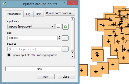
After running the script, the resulting layer will be loaded into QGIS and listed using the output parameter name; in this case, the layer is called squares. The following screenshot shows the automatically generated input dialog as well as the output of the script when applied to the airports from our sample dataset:
Especially when executing complex scripts that take a while to finish, it is good practice to display the progress of the script execution in a progress bar. To add a progress bar to the previous script, we can add the following lines of code before and inside the for loop that loops through the input features:
i = 0
n = my_layer.featureCount()
for input_feature in my_layer.getFeatures():
    progress.setPercentage(int(100*i/n))
    i+=1