Chapter 5. Demonstrating Change

In this chapter, we will encounter the visualization and analytical techniques of exploring the relationships between place and time and between the places themselves.

The data derived from temporal and spatial relationships is useful in learning more about the geographic objects that we are studying—from hydrological features to population units. This is particularly true if the data is not directly available for the geographic object of interest: either for a particular variable, for a particular time, or at all.

In this example, we will look at the demographic data from the US Census applied to the State House Districts, for election purposes. Elected officials often want to understand how the neighborhoods in their jurisdictions are changing demographically. Are their constituents becoming younger or more affluent? Is unemployment rising? Demographic factors can be used to predict the issues that will be of interest to potential voters and thus may be used for promotional purposes by the campaigns.

In this chapter, we will cover the following topics:

Using spatial relationships to leverage data
Preparing data relationships for static production
Vector simplification
Using TopoJSON for vector data size reduction and performance
D3 data visualization for API
Animated time series maps

Leveraging spatial relationships

So far, we've looked at the methods of analysis that take advantage of the continuity of the gridded raster data or of the geometric formality of the topological network data.

For ordinary vector data, we need a more abstract method of analysis, which is establishing the formal relationships based on the conditions in the spatial arrangement of geometric objects.

For most of this section, we will gather and prepare the data in ways that will be familiar. When we get to preparing the boundary data, which is leveraging the State House Districts data from the census tracts, we will be covering new territory—using the spatial relationships to construct the data for a given geographic unit.

Gathering the data

First, we will gather data from the sections of the US Census website. Though this workflow will be particularly useful for those working with the US demographic data, it will also be instructive for those dealing with any kind of data linked to geographic boundaries.

To begin with, obtain the boundary data with a unique identifier. After doing this, obtain the tabular data with the same unique identifier and then join on the identifier.

Boundaries

Download 2014 TIGER/Line Census Tracts and State Congressional Districts from the US Census at https://www.census.gov/geo/maps-data/data/tiger-line.html.

Select 2014 from the tabs displayed; this should be the default year.
Click on the Download accordion heading and click on Web interface.
Under Select a layer type, select Census Tracts and click on submit; under Census Tract, select Pennsylvania and click on Download.
Use the back arrow if necessary to select State Legislative Districts, and click on submit; select Pennsylvania for State Legislative Districts - Lower Chamber (current) and click on Download.
Move both the directories to c5/data/original and extract them.

Tip

We've only downloaded a single boundary dataset for this exercise. Since the boundaries are not consistent every year, you would want to download and work further with each separate annual boundary file in an actual project.

Tabular data from American FactFinder

Many different demographic datasets are available on the American FactFinder site. These complement the TIGER/Line data mentioned before with the attribute data for the TIGER/Line geographic boundaries. The main trick is to select the matching geographic boundary level and extent between the attribute and the geographic boundary data. Perform the following steps:

Go to the US Census American FactFinder site at http://factfinder.census.gov.
Click on the ADVANCED SEARCH tab.
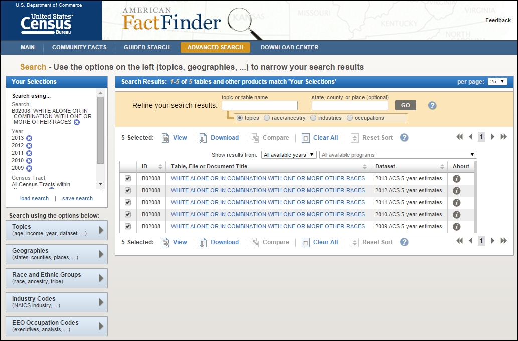
In the topic or table name input, enter White and select B02008: WHITE ALONE OR IN COMBINATION WITH ONE OR MORE RACES in the suggested options. Then, click on GO.
From the sidebar, in the Select a geographic type: dropdown in the Geographies section, select Census Tract - 140.
Under select a state, select Pennsylvania; under Select a county, select Philadelphia; and under Select one or more geographic areas and click Add to Your Selections:, select All Census Tracts within Philadelphia County, Pennsylvania. Then, click on ADD TO YOUR SELECTIONS.
From the sidebar, go to the Topics section. Here, in the Select Topics to add to 'Your Selections' under Year, click on each year available from 2009 to 2013, adding each to Your Selections to be then downloaded.
Check each of the five datasets offered under the Search Results tab. All checked datasets are added to the selection to be downloaded, as shown in the following screenshot:
Now, remove B02008: WHITE ALONE OR IN COMBINATION WITH ONE OR MORE RACES from the search filter showing selections in the upper-left corner of the page.
Enter total into the topic or table name field, selecting B01003: TOTAL POPULATION from the suggested datasets, and then click on GO.
Select the five 2009 to 2013 total population 5-year estimates and then click on GO.
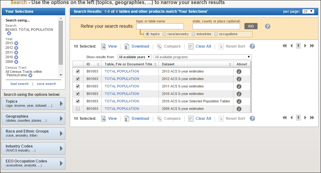
Click on Download to download these 10 datasets, as shown in the preceding screenshot.
Once you see the Your file is complete message, click on DOWNLOAD again to download the files. These will download as a aff_download.zip directory.
Move this directory to c5/data/original and then extract it.

Preparing and exporting the data

First, we will cover the steps for tabular data preparation and exporting, which are fairly similar to those we've done before. Next, we will cover the steps for preparing the boundary data, which will be more novel. We need to prepare this data based on the spatial relationships between layers, requiring the use of SQLite, since this cannot easily be done with the out-of-the-box or plugin functionality in QGIS.

The tabular data

Our tabular data is of the census tract white population. We only need to have the parseable latitude and longitude fields in this data for plotting later and, therefore, can leave it in this generic tabular format.

Combining it yearly

To combine this yearly data, we can join each table on a common GEOID field in QGIS. Perform the following steps:

Open QGIS and import all the boundary shapefiles (the tracts and state house boundaries) and data tables (all the census tract years downloaded). The single boundary shapefile will be in its extracted directory with the .shp extension. Data tables will be named something similar to x_with_ann.csv. You need to do this the same way you did earlier, which was through Add Vector Layer under the Layer menu. Here is a list of all the files to add:
- tl_2014_42_tract.shp
- ACS_09_5YR B01003_with_ann.csv
- ACS_10_5YR B01003_with_ann.csv
- ACS_11_5YR B01003_with_ann.csv
- ACS_12_5YR B01003_with_ann.csv
- ACS_13_5YR B01003_with_ann.csv
Select the tract boundaries shapefile, tl_2014_42_tract, from the Layers panel.
Navigate to Layers | Properties.
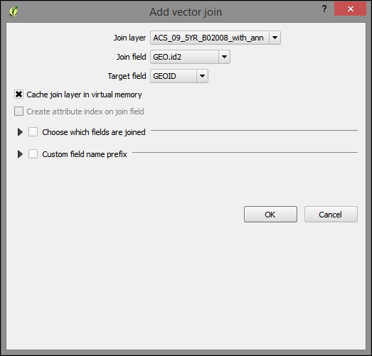
For each white population data table (ending in x_B02008_with_ann), perform the following steps:
1. On the Joins tab, click on the green plus sign (+) to add a join.
2. Select a data table as the Join layer.
3. Select GEO.id2 in the Join field tab.
4. Target field: GEOID

After joining all the tables, you will find many rows in the attribute table containing null values. If you sort them a few years later, you will find that we have the same number of rows populated for more recent years as we have in the Philadelphia tracts layer. However, the year 2009 (ACS_09_5YR B01003_with_ann.csv) has many rows that could not be populated due to the changes in the unique identifier used in the 2014 boundary data. For this reason, we will exclude the year 2009 from our analysis. You can remove the 2009 data table from the joined tables so that we don't have any issue with this later.

Now, export the joined layer as a new DBF database file, which we need to do to be able to make some final changes:

Ensure that only the rows with the populated data columns are selected in the tracts layer. Attribute the table (you can do this by sorting the attribute table on that field, for example).
Select the tracts layer from the Layers panel.
Navigate to Layer | Save as, fulfilling the following parameters:
- Format: DBF File
- Save only the selected features
- Add the saved file to the map
- Save as: c5/data/output/whites.dbf
- Leave the other options as they are by default

Updating and removing fields

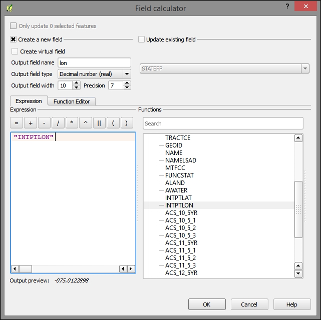
QGIS allows us to calculate the coordinates for the geographic features and populate an attribute field with them. On the layer for the new DBF, calculate the latitude and longitude fields in the expected format and eliminate the unnecessary fields by performing the following steps:

Open the Attribute table for the whites DBF layer and click on the Open Field Calculator button.
Calculate a new lon field and fulfill the following parameters:
- Output field name: lon.
- Output field type: Decimal number (real).
- Output field width: 10.
- Precision: 7.
- Expression: "INTPLON". You can choose this from the Fields and Values sections in the tree under the Functions panel.
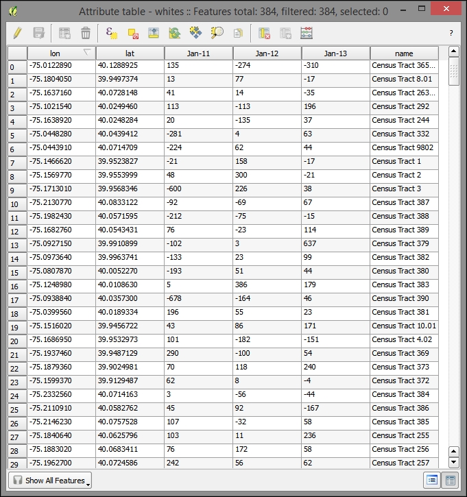
Repeat these steps with latitude, making a lat field from INTPLAT.
Create the following fields using the field calculator with the expression on the right:
- Output field name: name; Output field type: Text; Output field width: 50; Expression: NAMESLAD
- Output field name: Jan-11; Output field type: Whole number (integer); Expression: "ACS_11_5_2" - "ACS_10_5_2"
- Output field name: Jan-12; Output field type: Whole number (integer); Expression: "ACS_12_5_2" - "ACS_11_5_2"
- Output field name: Jan-13; Output field type: Whole number (integer); Expression: "ACS_13_5_2" - "ACS_12_5_2"
Remove all the old fields (except name, Jan-11, Jan-12, Jan-13, lat, and lon). This will remove all the unnecessary identification fields and those with a margin of error from the table.
Toggle the editing mode and save when prompted.

Finally, export the modified table as a new CSV data table, from which we will create our map visualization. Perform the following steps:

Select the whites DBF layer from the Layers panel.
Navigate to Layer | Save as while fulfilling the following parameters:
- Format: Comma Separated Value [CSV]
- Save as: c5/data/output/whites.csv
- Leave the other options as they were by default

The boundary data

Although we have the boundary data for the census tracts, we are only interested in visualizing the State House Districts in our application. Our stakeholders are interested in visualizing change for these districts. However, as we do not have the population data by race for these boundary units, let alone by the yearly population, we need to leverage the spatial relationship between the State House Districts and the tracts to derive this information. This is a useful workflow whenever you have the data at a different level than the geographic unit you wish to visualize or query.

Calculating the average white population change in each census tract

Now, we will construct a field that contains the average yearly change in the white population between 2010 and 2013. Perform the following steps:

As mentioned previously, join the total population tables (ending in B01003_with_ann) to the joined tract layer, tl_2014_42_tract, on the same GEO.id2, GEO fields from the new total population tables, and the tract layer respectively. Do not join the 2009 table, because we discovered that there were many null values in the join fields for the white-only version of this.
As before, select the 384 rows in the attribute table having the populated join columns from this table. Save only the selected rows, calling the saved shapefile dataset tract_change and adding this to the map.
Open the Attribute table and then open Field Calculator.
- Create a new field.
- Output field name: avg_change.
- Output field type: Decimal number (real).
- Output field width: 4, Precision: 2.
- The following expression is the difference of each year from the previous year divided by the previous year to find the fractional change. This is then divided by three to find the average over three years and finally multiplied by 100 to find the percentage, as follows:
```
((("ACS_11_5_2" - "ACS_10_5_2")/ "ACS_10_5_2" )+
  (("ACS_12_5_2" - "ACS_11_5_2")/ "ACS_11_5_2" )+
  (("ACS_13_5_2" - "ACS_12_5_2")/ "ACS_12_5_2" ))/3 * 100
```
After this, click on OK.

The spatial join in SpatiaLite

Now that we have a value for the average change in white population by tract, let's attach this to the unit of interest, which are the State House Districts. We will do this by doing a spatial join, specifically by joining all the records that intersect our House District bounds to that House District. As more than one tract will intersect each State House District, we'll need to aggregate the attribute data from the intersected tracts to match with the single district that the tracts will be joined to.

We will use SpatiaLite for doing this. Similar to PostGIS for Postgres, SpatiaLite is the spatial extension for SQLite. It is file-based; rather than requiring a continuous server listening for connections, a database is stored on a file, and client programs directly connect to it. Also, SpatiaLite comes with QGIS out of the box, making it very easy to begin to use. As with PostGIS, SpatiaLite comes with a rich set of spatial relationship functions, making it a good choice when the existing plugins do not support the relationship we are trying to model.

Tip

SpatiaLite is usually not chosen as a database for live websites because of some limitations related to multiuser transactions—which is why CartoDB uses Postgres as its backend database.

Creating a SpatiaLite database

To do this, perform the following steps:

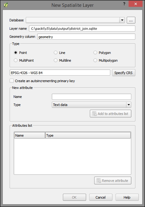
Create a new SpatiaLite database.
Navigate to Layer | Create Layer | New Spatialite Layer.
Using the ellipses button (…), browse to and create a database at c5/data/output/district_join.sqlite.
After clicking on Save, you will be notified that a new database has been registered. You have now created a new SpatiaLite database. You can now close this dialog.

Importing layers to SpatiaLite

To import layers to SpatiaLite, you can perform the following steps:

Navigate to Database | DB Manager | DB Manage.
Click on the refresh button. The new database should now be visible under the SpatiaLite section of the tree.
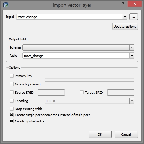
Navigate to Table | Import layer/file (tract_change and tl_2014_42_sldl).
Click on Update options.
Select Create single-part geometries instead of multi-part.
Select Create spatial index.
Click on OK to finish importing the table to the database (you may need to hit the refresh button again for table to be indicated as imported).

Now, repeat these steps with the House Districts layer (tl_2014_42_sldl), and deselect Create single-part geometries instead of multi-part as this seems to cause an error with this file, perhaps due to some part of a multi-part feature that would not be able to remain on its own under the SpatiaLite data requirements.

Querying and loading the SpatiaLite layer from the DB Manager

Next, we use the DB Manager to query the SpatiaLite database, adding the results to the QGIS layers panel.

We will use the MBRIntersects criteria here, which provides a performance advantage over a regular Intersects function as it only checks for the intersection of the extent (bounding box). In this example, we are dealing with a few features of limited complexity that are not done dynamically during a web request, so this shortcut does not provide a major advantage—we do this here so as to demonstrate its use for more complicated datasets.

If it isn't already open, open DB Manager.
Navigate to Database | SQL window.
- Fill the respective input fields in the SQL query dialog:
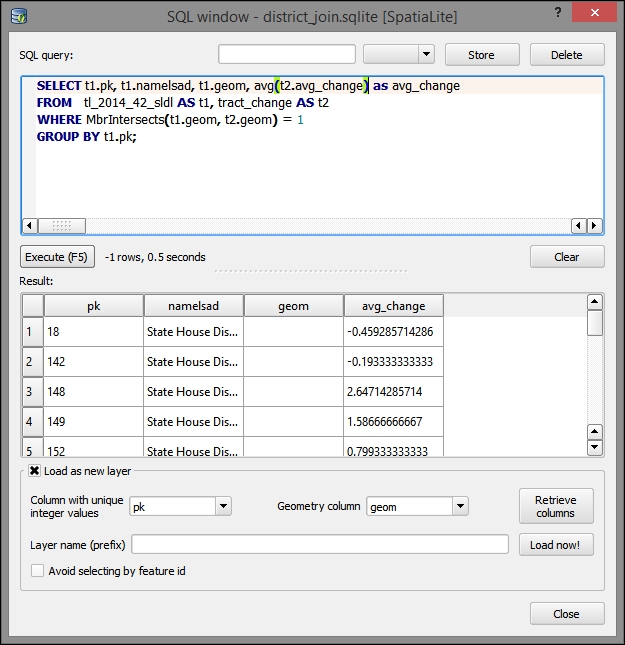
- The following SQL query selects the fields from the tract_change and tl_2014_42_sldl (State Legislative District) tables, where they overlap. It also performs an aggregate (average) of the change by the State Legislative Districts overlying the census tract boundaries:
```
SELECT t1.pk, t1.namelsad, t1.geom, avg(t2.avg_change)*1.0 as avg_change
FROM   tl_2014_42_sldl AS t1, tract_change AS t2
WHERE MbrIntersects(t1.geom, t2.geom) = 1
GROUP BY t1.pk;
```
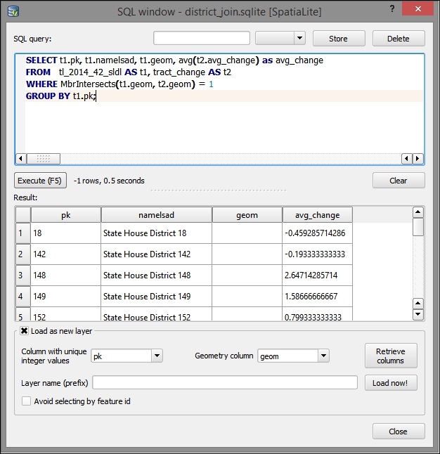
Then, click on Load now!.
You will be prompted to select a value for the Column with unique integer values field. For this, select pk.
You will also be prompted to select a value for the Geometry column field; for this, select geom.

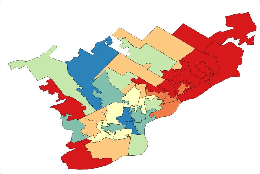
The symbolized result of the spatial relationship join showing the average white population change over a 4-year period for the State House Districts' census tracts intersection will look something similar to the following image: