Table of Contents for
QGIS: Becoming a GIS Power User
 QGIS: Becoming a GIS Power User
Published by
Packt Publishing, 2017
QGIS: Becoming a GIS Power User
Published by
Packt Publishing, 2017
- Cover
- Table of Contents
- QGIS: Becoming a GIS Power User
- QGIS: Becoming a GIS Power User
- QGIS: Becoming a GIS Power User
- Credits
- Preface
- What you need for this learning path
- Who this learning path is for
- Reader feedback
- Customer support
- 1. Module 1
- 1. Getting Started with QGIS
- Running QGIS for the first time
- Introducing the QGIS user interface
- Finding help and reporting issues
- Summary
- 2. Viewing Spatial Data
- Dealing with coordinate reference systems
- Loading raster files
- Loading data from databases
- Loading data from OGC web services
- Styling raster layers
- Styling vector layers
- Loading background maps
- Dealing with project files
- Summary
- 3. Data Creation and Editing
- Working with feature selection tools
- Editing vector geometries
- Using measuring tools
- Editing attributes
- Reprojecting and converting vector and raster data
- Joining tabular data
- Using temporary scratch layers
- Checking for topological errors and fixing them
- Adding data to spatial databases
- Summary
- 4. Spatial Analysis
- Combining raster and vector data
- Vector and raster analysis with Processing
- Leveraging the power of spatial databases
- Summary
- 5. Creating Great Maps
- Labeling
- Designing print maps
- Presenting your maps online
- Summary
- 6. Extending QGIS with Python
- Getting to know the Python Console
- Creating custom geoprocessing scripts using Python
- Developing your first plugin
- Summary
- 2. Module 2
- 1. Exploring Places – from Concept to Interface
- Acquiring data for geospatial applications
- Visualizing GIS data
- The basemap
- Summary
- 2. Identifying the Best Places
- Raster analysis
- Publishing the results as a web application
- Summary
- 3. Discovering Physical Relationships
- Spatial join for a performant operational layer interaction
- The CartoDB platform
- Leaflet and an external API: CartoDB SQL
- Summary
- 4. Finding the Best Way to Get There
- OpenStreetMap data for topology
- Database importing and topological relationships
- Creating the travel time isochron polygons
- Generating the shortest paths for all students
- Web applications – creating safe corridors
- Summary
- 5. Demonstrating Change
- TopoJSON
- The D3 data visualization library
- Summary
- 6. Estimating Unknown Values
- Interpolated model values
- A dynamic web application – OpenLayers AJAX with Python and SpatiaLite
- Summary
- 7. Mapping for Enterprises and Communities
- The cartographic rendering of geospatial data – MBTiles and UTFGrid
- Interacting with Mapbox services
- Putting it all together
- Going further – local MBTiles hosting with TileStream
- Summary
- 3. Module 3
- 1. Data Input and Output
- Finding geospatial data on your computer
- Describing data sources
- Importing data from text files
- Importing KML/KMZ files
- Importing DXF/DWG files
- Opening a NetCDF file
- Saving a vector layer
- Saving a raster layer
- Reprojecting a layer
- Batch format conversion
- Batch reprojection
- Loading vector layers into SpatiaLite
- Loading vector layers into PostGIS
- 2. Data Management
- Joining layer data
- Cleaning up the attribute table
- Configuring relations
- Joining tables in databases
- Creating views in SpatiaLite
- Creating views in PostGIS
- Creating spatial indexes
- Georeferencing rasters
- Georeferencing vector layers
- Creating raster overviews (pyramids)
- Building virtual rasters (catalogs)
- 3. Common Data Preprocessing Steps
- Converting points to lines to polygons and back – QGIS
- Converting points to lines to polygons and back – SpatiaLite
- Converting points to lines to polygons and back – PostGIS
- Cropping rasters
- Clipping vectors
- Extracting vectors
- Converting rasters to vectors
- Converting vectors to rasters
- Building DateTime strings
- Geotagging photos
- 4. Data Exploration
- Listing unique values in a column
- Exploring numeric value distribution in a column
- Exploring spatiotemporal vector data using Time Manager
- Creating animations using Time Manager
- Designing time-dependent styles
- Loading BaseMaps with the QuickMapServices plugin
- Loading BaseMaps with the OpenLayers plugin
- Viewing geotagged photos
- 5. Classic Vector Analysis
- Selecting optimum sites
- Dasymetric mapping
- Calculating regional statistics
- Estimating density heatmaps
- Estimating values based on samples
- 6. Network Analysis
- Creating a simple routing network
- Calculating the shortest paths using the Road graph plugin
- Routing with one-way streets in the Road graph plugin
- Calculating the shortest paths with the QGIS network analysis library
- Routing point sequences
- Automating multiple route computation using batch processing
- Matching points to the nearest line
- Creating a routing network for pgRouting
- Visualizing the pgRouting results in QGIS
- Using the pgRoutingLayer plugin for convenience
- Getting network data from the OSM
- 7. Raster Analysis I
- Using the raster calculator
- Preparing elevation data
- Calculating a slope
- Calculating a hillshade layer
- Analyzing hydrology
- Calculating a topographic index
- Automating analysis tasks using the graphical modeler
- 8. Raster Analysis II
- Calculating NDVI
- Handling null values
- Setting extents with masks
- Sampling a raster layer
- Visualizing multispectral layers
- Modifying and reclassifying values in raster layers
- Performing supervised classification of raster layers
- 9. QGIS and the Web
- Using web services
- Using WFS and WFS-T
- Searching CSW
- Using WMS and WMS Tiles
- Using WCS
- Using GDAL
- Serving web maps with the QGIS server
- Scale-dependent rendering
- Hooking up web clients
- Managing GeoServer from QGIS
- 10. Cartography Tips
- Using Rule Based Rendering
- Handling transparencies
- Understanding the feature and layer blending modes
- Saving and loading styles
- Configuring data-defined labels
- Creating custom SVG graphics
- Making pretty graticules in any projection
- Making useful graticules in printed maps
- Creating a map series using Atlas
- 11. Extending QGIS
- Defining custom projections
- Working near the dateline
- Working offline
- Using the QspatiaLite plugin
- Adding plugins with Python dependencies
- Using the Python console
- Writing Processing algorithms
- Writing QGIS plugins
- Using external tools
- 12. Up and Coming
- Preparing LiDAR data
- Opening File Geodatabases with the OpenFileGDB driver
- Using Geopackages
- The PostGIS Topology Editor plugin
- The Topology Checker plugin
- GRASS Topology tools
- Hunting for bugs
- Reporting bugs
- Bibliography
- Index
Although the data has been added to the GIS through the ETL process, it is of limited value without adding some visualization enhancements.
The layer style is configured through the Style tab in the Layer Properties dialog. The Single Symbol style is the default style type, and it simply shows all the geographic layer objects using the same basic symbol. This setting doesn't provide any visual differentiation between objects other than their apparent geospatial characteristics. The Categorized and Graduated style types provide different styles according to the attribute table field of your choosing. Graduated, which applies to quantitative data, is particularly powerful in the way the color and symbols size are mapped to a numerical scale. This is all accomplished through the Layer Properties | Style tab.
To configure a simple graduated layer style to the data, perform the following steps:
- Under the Layer Properties | Style tab, select Graduated for the style type.
- Select your quantitative field for Column (such as
temperature_mean_temp). - Click on Classify to group your data into the number of classes specified (by default, 5) and to select the classification mode (Equal Interval, by default):
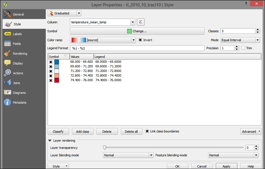
- Now, click on Apply.
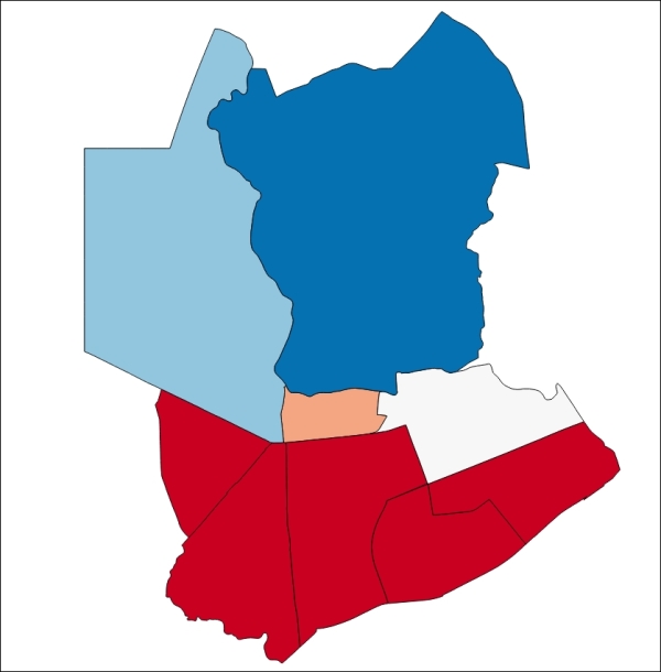
If you applied the preceding steps to the joined tract/temperature layer, you'd see something similar to the following image:
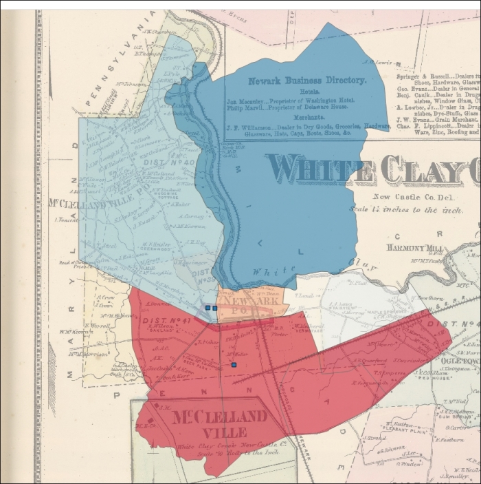
- You can add some layer transparency here if you'd like to simultaneously view other layers. This would be appropriate if this layer were to be included in a basemap.
- Now, click on OK.
You will now see the following output:
Perhaps the lower temperatures to the north of the city are related to the historical development in other parts of the city.
Labels can provide important information in a map without requiring a popup or legend. As labels are automatically placed by the software (they do not have an actual physical position in space), they are subject to particular placement issues. Also, a map with too much label text quickly becomes confusing. Sometimes, labels can be easily rendered into tiles by integrated QGIS operations. At other times, this will require an external rendering engine or a map server. These issues are discussed later on in this chapter.
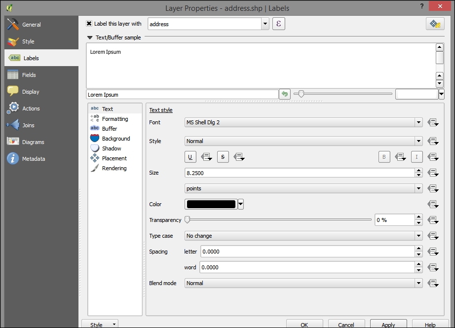
To label the address points in our example, go to that layer's Layer Properties | Labels tab. Perform the following steps:
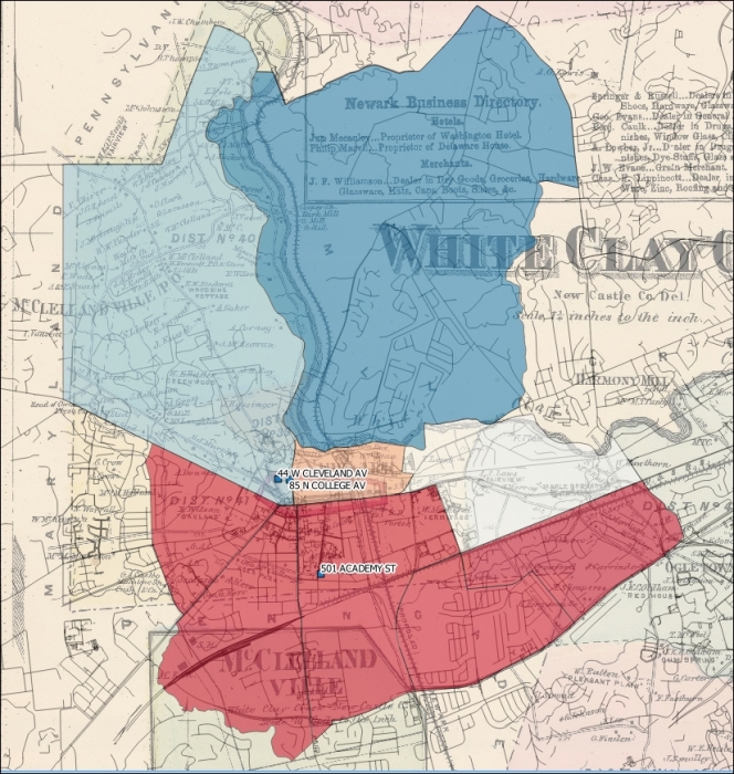
- Select address for the Label this layer with field. Note that the checkbox next to this selection will be toggled. All other label style options will remain the same, as shown in the following screenshot:
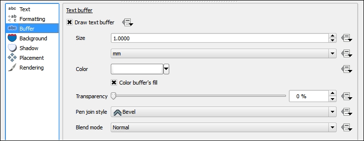
- Open the Buffer subtab and toggle Draw text buffer:
- After you click on OK, you will see something similar to the following screenshot: