Vector and raster analysis with Processing

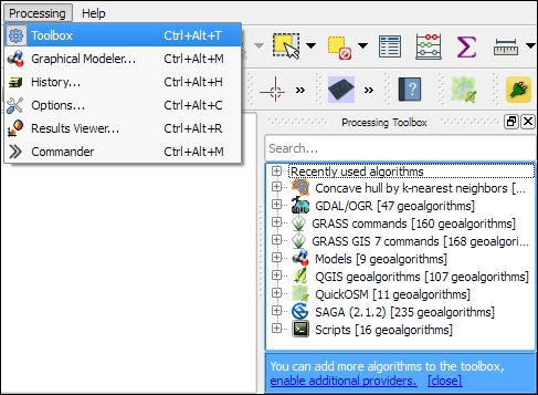
The most comprehensive set of spatial analysis tools is accessible via the Processing plugin, which we can enable in the Plugin Manager. When this plugin is enabled, we find a Processing menu, where we can activate the Toolbox, as shown in the following screenshot. In the toolbox, it is easy to find spatial analysis tools by their name thanks to the dynamic Search box at the top. This makes finding tools in the toolbox easier than in the Vector or Raster menu. Another advantage of getting accustomed to the Processing tools is that they can be automated in Python and in geoprocessing models.

In the following sections, we will cover a selection of the available geoprocessing tools and see how we can use the modeler to automate our tasks.

Finding nearest neighbors

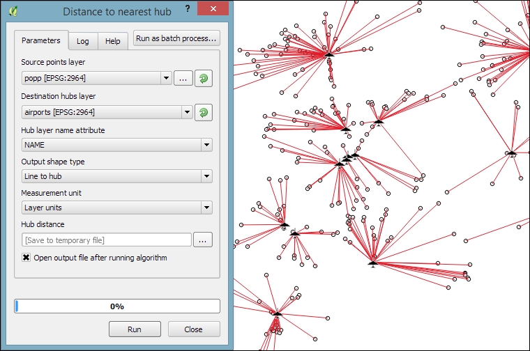
Finding nearest neighbors, for example, the airport nearest to a populated place, is a common task in geoprocessing. To find the nearest neighbor and create connections between input features and their nearest neighbor in another layer, we can use the Distance to nearest hub tool.

As shown in the next screenshot, we use the populated places as Source points layer and the airports as the Destination hubs layer. The Hub layer name attribute will be added to the result's attribute table to identify the nearest feature. Therefore, we select NAME to add the airport name to the populated places. There are two options for Output shape type:

Point: This option creates a point output layer with all points of the source point layer, with new attributes for the nearest hub feature and the distance to it
Line to hub: This option creates a line output layer with connections between all points of the source point layer and their corresponding nearest hub feature

It is recommended that you use Layer units as Measurement unit to avoid potential issues with wrong measurements:

Converting between points, lines, and polygons

It is often necessary to be able to convert between points, lines, and polygons, for example, to create lines from a series of points, or to extract the nodes of polygons and create a new point layer out of them. There are many tools that cover these different use cases. The following table provides an overview of the tools that are available in the Processing toolbox for conversion between points, lines, and polygons:

	To points	To lines	To polygons
From points		Points to path	Convex hull Concave hull
From lines	Extract nodes		Lines to polygons Convex hull
From polygons	Extract nodes Polygon centroids (Random points inside a polygon)	Polygons to lines

To points

To lines

To polygons

From points

Points to path

Convex hull

Concave hull

From lines

Extract nodes

Lines to polygons

Convex hull

From polygons

Extract nodes

Polygon centroids

(Random points inside a polygon)

Polygons to lines

In general, it is easier to convert more complex representations to simpler ones (polygons to lines, polygons to points, or lines to points) than conversion in the other direction (points to lines, points to polygons, or lines to polygons). Here is a short overview of these tools:

Extract nodes: This is a very straightforward tool. It takes one input layer with lines or polygons and creates a point layer that contains all the input geometry nodes. The resulting points contain all the attributes of the original line or polygon feature.
Polygon centroids: This tool creates one centroid per polygon or multipolygon. It is worth noting that it does not ensure that the centroid falls within the polygon. For concave polygons, multipolygons, and polygons with holes, the centroid can therefore fall outside the polygon.
Random points inside polygon: This tool creates a certain number of points at random locations inside the polygon.
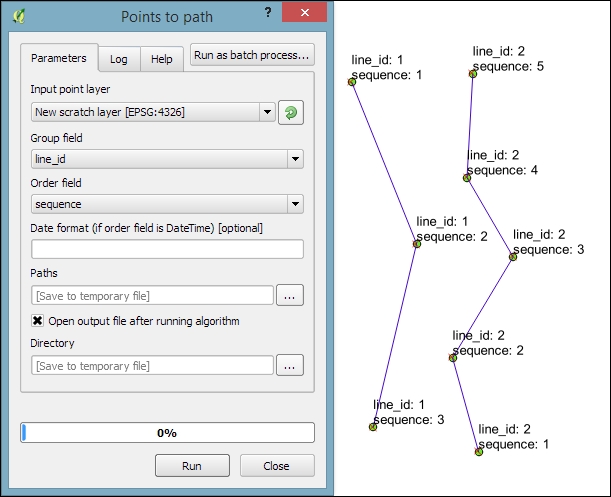
Points to path: To be able to create lines from points, the point layer needs attributes that identify the line (Group field) and the order of points in the line (Order field), as shown in this screenshot:
Convex hull: This tool creates a convex hull around the input points or lines. The convex hull can be imagined as an area that contains all the input points as well as all the connections between the input points.
Concave hull: This tool creates a concave hull around the input points. The concave hull is a polygon that represents the area occupied by the input points. The concave hull is equal to or smaller than the convex hull. In this tool, we can control the level of detail of the concave hull by changing the Threshold parameter between 0 (very detailed) and 1 (which is equivalent to the convex hull). The following screenshot shows a comparison between convex and concave hulls (with the threshold set to 0.3) around our airport data:
Lines to polygon: Finally, this tool can create polygons from lines that enclose an area. Make sure that there are no gaps between the lines. Otherwise, it will not work.

Identifying features in the proximity of other features

One common spatial analysis task is to identify features in the proximity of certain other features. One example would be to find all airports near rivers. Using airports.shp and majrivers.shp from our sample data, we can find airports within 5,000 feet of a river by using a combination of the Fixed distance buffer and Select by location tools. Use the search box to find the tools in the Processing Toolbox. The tool configurations for this example are shown in the following screenshot:

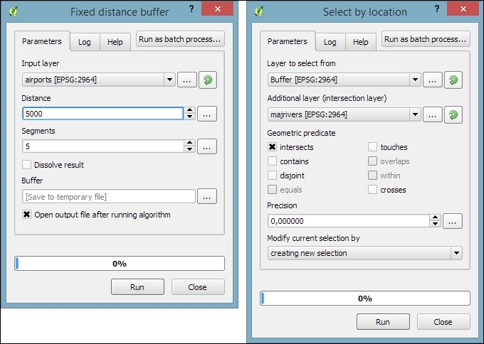
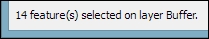
After buffering the airport point locations, the Select by location tool selects all the airport buffers that intersect a river. As a result, 14 out of the 76 airports are selected. This information is displayed in the information area at the bottom of the QGIS main window, as shown in this screenshot:

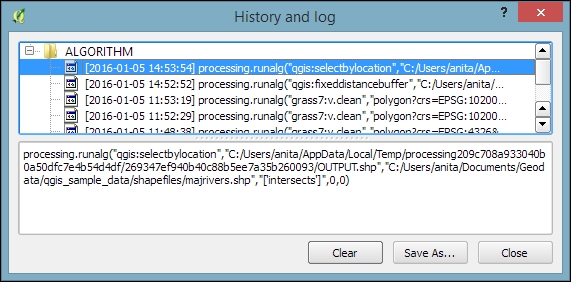
If you ever forget which settings you used or need to check whether you have used the correct input layer, you can go to Processing | History. The ALGORITHM section lists all the algorithms that we have been running as well as the used settings, as shown in the following screenshot:

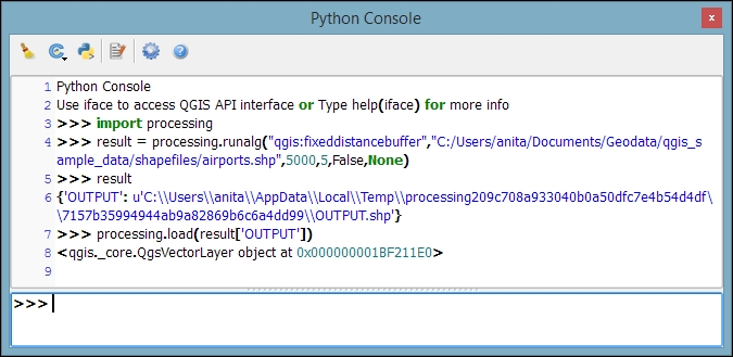
The commands listed under ALGORITHM can also be used to call Processing tools from the QGIS Python console, which can be activated by going to Plugins | Python Console. The Python commands shown in the following screenshot run the buffer algorithm (processing.runalg) and load the result into the map (processing.load):

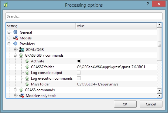
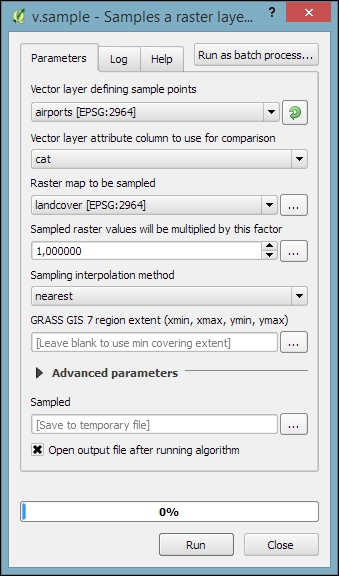
Sampling a raster at point locations

Another common task is to sample a raster at specific point locations. Using Processing, we can solve this problem with a GRASS tool called v.sample. To use GRASS tools, make sure that GRASS is installed and Processing is configured correctly under Processing | Options and configuration. On an OSGeo4W default system, the configuration will look like what is shown here:

Note

At the time of writing this book, GRASS 7.0.3RC1 is available in OSGeo4W. As shown in the previous screenshot, there is also support for the previous GRASS version 6.x, and Processing can be configured to use its algorithms as well. In the toolbox, you will find the algorithms under GRASS GIS 7 commands and GRASS commands (for GRASS 6.x).

For this exercise, let's imagine we want to sample the landcover layer at the airport locations of our sample data. All we have to do is specify the vector layer containing the sample points and the raster layer that should be sampled. For this example, we can leave all other settings at their default values, as shown in the following screenshot. The tool not only samples the raster but also compares point attributes with the sampled raster value. However, we don't need this comparison in our current example:

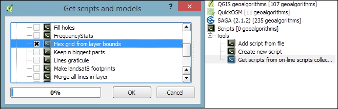
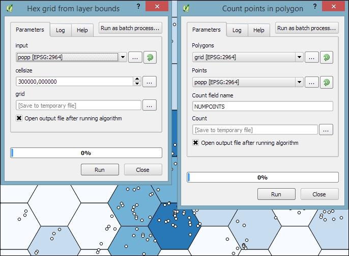
Mapping density with hexagonal grids

Mapping the density of points using a hexagonal grid has become quite a popular alternative to creating heatmaps. Processing offers us a fast way to create such an analysis. There is already a pre-made script called Hex grid from layer bounds, which is available through the Processing scripts collection and can be downloaded using the Get scripts from on-line scripts collection tool. As you can see in the following screenshot, you just need to enable the script by ticking the checkbox and clicking OK:

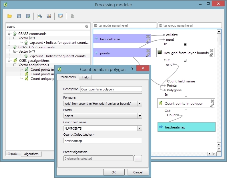
Then, we can use this script to create a hexagonal grid that covers all points in the input layer. The dataset of populated places (popp.shp), is a good sample dataset for this exercise. Once the grid is ready, we can run Count points in polygon to calculate the statistics. The number of points will be stored in the NUMPOINTS column if you use the settings shown in the following screenshot:

Calculating area shares within a region

Another spatial analysis task we often encounter is calculating area shares within a certain region, for example, landcover shares along one specific river. Using majrivers.shp and trees.shp, we can calculate the share of wooded area in a 10,000-foot-wide strip of land along the Susitna River:

We first define the analysis region by selecting the river and buffering it.
Tip
QGIS Processing will only apply buffers to the selected features of the input layer. This default behavior can be changed under Processing | Options and configuration by disabling the Use only selected features option. For the following examples, please leave the option enabled.
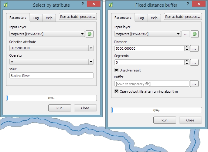
To select the Susitna River, we use the Select by attribute tool. After running the tool, you should see that our river of interest is selected and highlighted.
Then we can use the Fixed distance buffer tool to get the area within 5,000 feet along the river. Note that the Dissolve result option should be enabled to ensure that the buffer result is one continuous polygon, as shown in the following screenshot:
Next, we calculate the size of the strip of land around our river. This can be done using the Export/Add geometry columns tool, which adds the area and perimeter to the attribute table.
Then, we can calculate the Intersection between the area along the river and the wooded areas in trees.shp, as shown in the following screenshot. The result of this operation is a layer that contains only those wooded areas within the river buffer.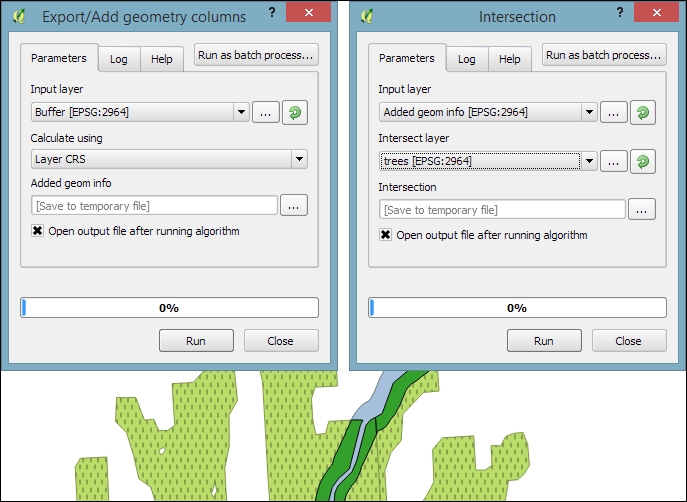
Using the Dissolve tool, we can recombine all areas from the intersection results into one big polygon that represents the total wooded area around the river. Note how we use the Unique ID field VEGDESC to only combine areas with the same vegetation in order not to mix deciduous and mixed trees.
Finally, we can calculate the final share of wooded area using the Advanced Python field calculator. The formula value = $geom.area()/<area> divides the area of the final polygon ($geom.area()) by the value in the area attribute (<area>), which we created earlier by running Export/Add geometry columns. As shown in the following screenshot, this calculation results in a wood share of 0.31601 for Deciduous and 0.09666 for Mixed Trees. Therefore, we can conclude that in total, 41.27 percent of the land along the Susitna River is wooded: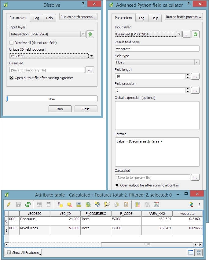

Batch-processing multiple datasets

Sometimes, we want to run the same tool repeatedly but with slightly different settings. For this use case, Processing offers the Batch Processing functionality. Let's use this tool to extract some samples from our airports layer using the Random extract tool:

To access the batch processing functionality, right-click on the Random extract tool in the toolbox and select Execute as batch process. This will open the Batch Processing dialog.
Next, we configure the Input layer by clicking on the ... button and selecting Select from open layers, as shown in the following screenshot:
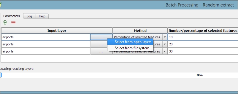
This will open a small dialog in which we can select the airports layer and click on OK.
To automatically fill in the other rows with the same input layer, we can double-click on the table header of the corresponding column (which reads Input layer).
Next, we configure the Method by selecting the Percentage of selected features option and again double-clicking on the respective table header to auto-fill the remaining rows.
The next parameter controls the Number/percentage of selected features. For our exercise, we configure 10, 20, and 30 percent.
Last but not least, we need to configure the output files in the Extracted (random) column. Click on the ... button, which will open a file dialog. There, you can select the save location and filename (for example, extract) and click on Save.
This will open the Autofill settings dialog, which helps us to automatically create distinct filenames for each run. Using the Fill with parameter values mode with the Number/percentage of selected features parameter will automatically append our parameter values (10, 20, and 30, respectively) to the filename. This will result in extract10, extract20, and extract30, as shown in the following screenshot: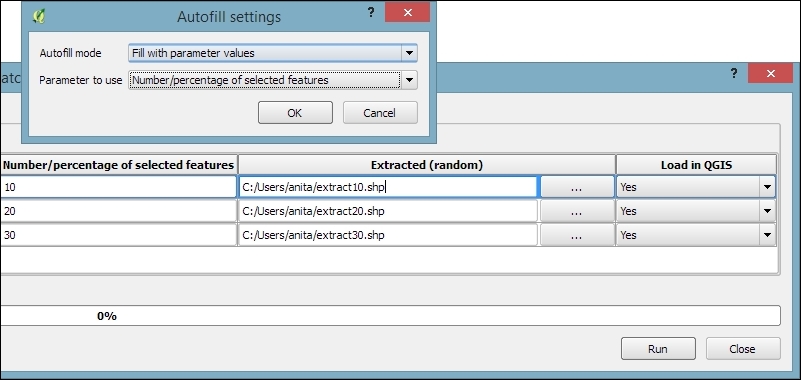
Once everything is configured, click on the Run button and wait for all the batch instructions to be processed and the results to be loaded into the project.

Automated geoprocessing with the graphical modeler

Using the graphical modeler, we can turn entire geoprocessing and analysis workflows into automated models. We can then use these models to run complex geoprocessing tasks that involve multiple different tools in one go. To create a model, we go to Processing | Graphical modeler to open the modeler, where we can select from different Inputs and Algorithms for our model.

Let's create a model that automates the creation of hexagonal heatmaps!

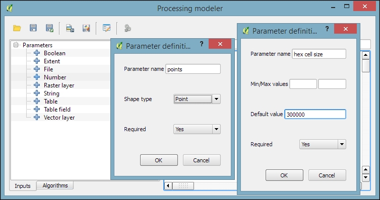
By double-clicking on the Vector layer entry in the Inputs list, we can add an input field for the point layer. It's a good idea to use descriptive parameter names (for example, hex cell size instead of just size for the parameter that controls the size of the hexagonal grid cells) so that we can recognize which input is first and which is later in the model. It is also useful to restrict the Shape type field wherever appropriate. In our example, we restrict the input to Point layers. This will enable Processing to pre-filter the available layers and present us only the layers of the correct type.
The second input that we need is a Number field to specify the desired hexagonal cell size, as shown in this screenshot:
After adding the inputs, we can now continue creating the model by assembling the algorithms. In the Algorithms section, we can use the filter at the top to narrow down our search for the correct algorithm. To add an algorithm to the model, we simply double-click on the entry in the list of algorithms. This opens the algorithm dialog, where we have to specify the inputs and further algorithm-specific parameters.
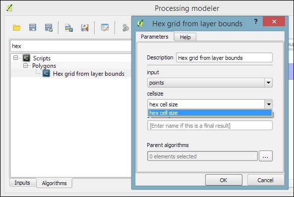
In our example, we want to use the point vector layer as the input layer and the number input hex cell size as the cellsize parameter. We can access the available inputs through the drop-down list, as shown in the following screenshot. Alternatively, it's possible to hardcode parameters such as the cell size by typing the desired value in the input field:
Tip
While adding the following algorithms, it is important to always choose the correct input layer based on the previous processing step. We can verify the workflow using the connections in the model diagram that the modeler draws automatically.
The final model will look like this:
To finish the model, we need to enter a model name (for example, Create hexagonal heatmap) and a group name (for example, Learning QGIS). Processing will use the group name to organize all the models that we create into different toolbox groups. Once we have picked a name and group, we can save the model and then run it.
After closing the modeler, we can run the saved models from the toolbox like any other tool. It is even possible to use one model as a building block for another model.

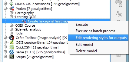
Another useful feature is that we can specify a layer style that needs to be applied to the processing results automatically. This default style can be set using Edit rendering styles for outputs in the context menu of the created model in the toolbox, as shown in the following screenshot:

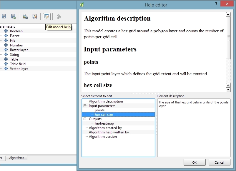
Automated geoprocessing with the graphical modeler

Documenting and sharing models

Models can easily be copied from one QGIS installation to another and shared with other users. To ensure the usability of the model, it is a good idea to write a short documentation. Processing provides a convenient Help editor; it can be accessed by clicking on the Edit model help button in the Processing modeler, as shown in this screenshot:

By default, the .model files are stored in your user directory. On Windows, it is C:\Users\<your_user_name>\.qgis2\processing\models, and on Linux and OS X, it is ~/.qgis2/processing/models.

You can copy these files and share them with others. To load a model from a file, use the loading tool by going to Models | Tools | Add model from file in the Processing Toolbox.

Previous Chapter

Combining raster and vector data

Next Chapter

Leveraging the power of spatial databases