Table of Contents for
QGIS: Becoming a GIS Power User
 QGIS: Becoming a GIS Power User
Published by
Packt Publishing, 2017
QGIS: Becoming a GIS Power User
Published by
Packt Publishing, 2017
- Cover
- Table of Contents
- QGIS: Becoming a GIS Power User
- QGIS: Becoming a GIS Power User
- QGIS: Becoming a GIS Power User
- Credits
- Preface
- What you need for this learning path
- Who this learning path is for
- Reader feedback
- Customer support
- 1. Module 1
- 1. Getting Started with QGIS
- Running QGIS for the first time
- Introducing the QGIS user interface
- Finding help and reporting issues
- Summary
- 2. Viewing Spatial Data
- Dealing with coordinate reference systems
- Loading raster files
- Loading data from databases
- Loading data from OGC web services
- Styling raster layers
- Styling vector layers
- Loading background maps
- Dealing with project files
- Summary
- 3. Data Creation and Editing
- Working with feature selection tools
- Editing vector geometries
- Using measuring tools
- Editing attributes
- Reprojecting and converting vector and raster data
- Joining tabular data
- Using temporary scratch layers
- Checking for topological errors and fixing them
- Adding data to spatial databases
- Summary
- 4. Spatial Analysis
- Combining raster and vector data
- Vector and raster analysis with Processing
- Leveraging the power of spatial databases
- Summary
- 5. Creating Great Maps
- Labeling
- Designing print maps
- Presenting your maps online
- Summary
- 6. Extending QGIS with Python
- Getting to know the Python Console
- Creating custom geoprocessing scripts using Python
- Developing your first plugin
- Summary
- 2. Module 2
- 1. Exploring Places – from Concept to Interface
- Acquiring data for geospatial applications
- Visualizing GIS data
- The basemap
- Summary
- 2. Identifying the Best Places
- Raster analysis
- Publishing the results as a web application
- Summary
- 3. Discovering Physical Relationships
- Spatial join for a performant operational layer interaction
- The CartoDB platform
- Leaflet and an external API: CartoDB SQL
- Summary
- 4. Finding the Best Way to Get There
- OpenStreetMap data for topology
- Database importing and topological relationships
- Creating the travel time isochron polygons
- Generating the shortest paths for all students
- Web applications – creating safe corridors
- Summary
- 5. Demonstrating Change
- TopoJSON
- The D3 data visualization library
- Summary
- 6. Estimating Unknown Values
- Interpolated model values
- A dynamic web application – OpenLayers AJAX with Python and SpatiaLite
- Summary
- 7. Mapping for Enterprises and Communities
- The cartographic rendering of geospatial data – MBTiles and UTFGrid
- Interacting with Mapbox services
- Putting it all together
- Going further – local MBTiles hosting with TileStream
- Summary
- 3. Module 3
- 1. Data Input and Output
- Finding geospatial data on your computer
- Describing data sources
- Importing data from text files
- Importing KML/KMZ files
- Importing DXF/DWG files
- Opening a NetCDF file
- Saving a vector layer
- Saving a raster layer
- Reprojecting a layer
- Batch format conversion
- Batch reprojection
- Loading vector layers into SpatiaLite
- Loading vector layers into PostGIS
- 2. Data Management
- Joining layer data
- Cleaning up the attribute table
- Configuring relations
- Joining tables in databases
- Creating views in SpatiaLite
- Creating views in PostGIS
- Creating spatial indexes
- Georeferencing rasters
- Georeferencing vector layers
- Creating raster overviews (pyramids)
- Building virtual rasters (catalogs)
- 3. Common Data Preprocessing Steps
- Converting points to lines to polygons and back – QGIS
- Converting points to lines to polygons and back – SpatiaLite
- Converting points to lines to polygons and back – PostGIS
- Cropping rasters
- Clipping vectors
- Extracting vectors
- Converting rasters to vectors
- Converting vectors to rasters
- Building DateTime strings
- Geotagging photos
- 4. Data Exploration
- Listing unique values in a column
- Exploring numeric value distribution in a column
- Exploring spatiotemporal vector data using Time Manager
- Creating animations using Time Manager
- Designing time-dependent styles
- Loading BaseMaps with the QuickMapServices plugin
- Loading BaseMaps with the OpenLayers plugin
- Viewing geotagged photos
- 5. Classic Vector Analysis
- Selecting optimum sites
- Dasymetric mapping
- Calculating regional statistics
- Estimating density heatmaps
- Estimating values based on samples
- 6. Network Analysis
- Creating a simple routing network
- Calculating the shortest paths using the Road graph plugin
- Routing with one-way streets in the Road graph plugin
- Calculating the shortest paths with the QGIS network analysis library
- Routing point sequences
- Automating multiple route computation using batch processing
- Matching points to the nearest line
- Creating a routing network for pgRouting
- Visualizing the pgRouting results in QGIS
- Using the pgRoutingLayer plugin for convenience
- Getting network data from the OSM
- 7. Raster Analysis I
- Using the raster calculator
- Preparing elevation data
- Calculating a slope
- Calculating a hillshade layer
- Analyzing hydrology
- Calculating a topographic index
- Automating analysis tasks using the graphical modeler
- 8. Raster Analysis II
- Calculating NDVI
- Handling null values
- Setting extents with masks
- Sampling a raster layer
- Visualizing multispectral layers
- Modifying and reclassifying values in raster layers
- Performing supervised classification of raster layers
- 9. QGIS and the Web
- Using web services
- Using WFS and WFS-T
- Searching CSW
- Using WMS and WMS Tiles
- Using WCS
- Using GDAL
- Serving web maps with the QGIS server
- Scale-dependent rendering
- Hooking up web clients
- Managing GeoServer from QGIS
- 10. Cartography Tips
- Using Rule Based Rendering
- Handling transparencies
- Understanding the feature and layer blending modes
- Saving and loading styles
- Configuring data-defined labels
- Creating custom SVG graphics
- Making pretty graticules in any projection
- Making useful graticules in printed maps
- Creating a map series using Atlas
- 11. Extending QGIS
- Defining custom projections
- Working near the dateline
- Working offline
- Using the QspatiaLite plugin
- Adding plugins with Python dependencies
- Using the Python console
- Writing Processing algorithms
- Writing QGIS plugins
- Using external tools
- 12. Up and Coming
- Preparing LiDAR data
- Opening File Geodatabases with the OpenFileGDB driver
- Using Geopackages
- The PostGIS Topology Editor plugin
- The Topology Checker plugin
- GRASS Topology tools
- Hunting for bugs
- Reporting bugs
- Bibliography
- Index
Transparency is a lack of pigment or color, such that you can see through one feature to the feature beneath. You can think of this as being similar to tinted or stained glass; some light is allowed to pass through and reflect off what's inside. When used right, transparency can help emphasize or de-emphasize features in a map composition. It can also be used to blend two layers to look as if they are one layer.
This recipe demonstrates transparency for both vectors and rasters, so we'll need an example of each. The lakes.shp and elevlid_D782_6.tif layers will work well for demonstration purposes. Load both of these layers in a fresh project, putting lake.shp on top.
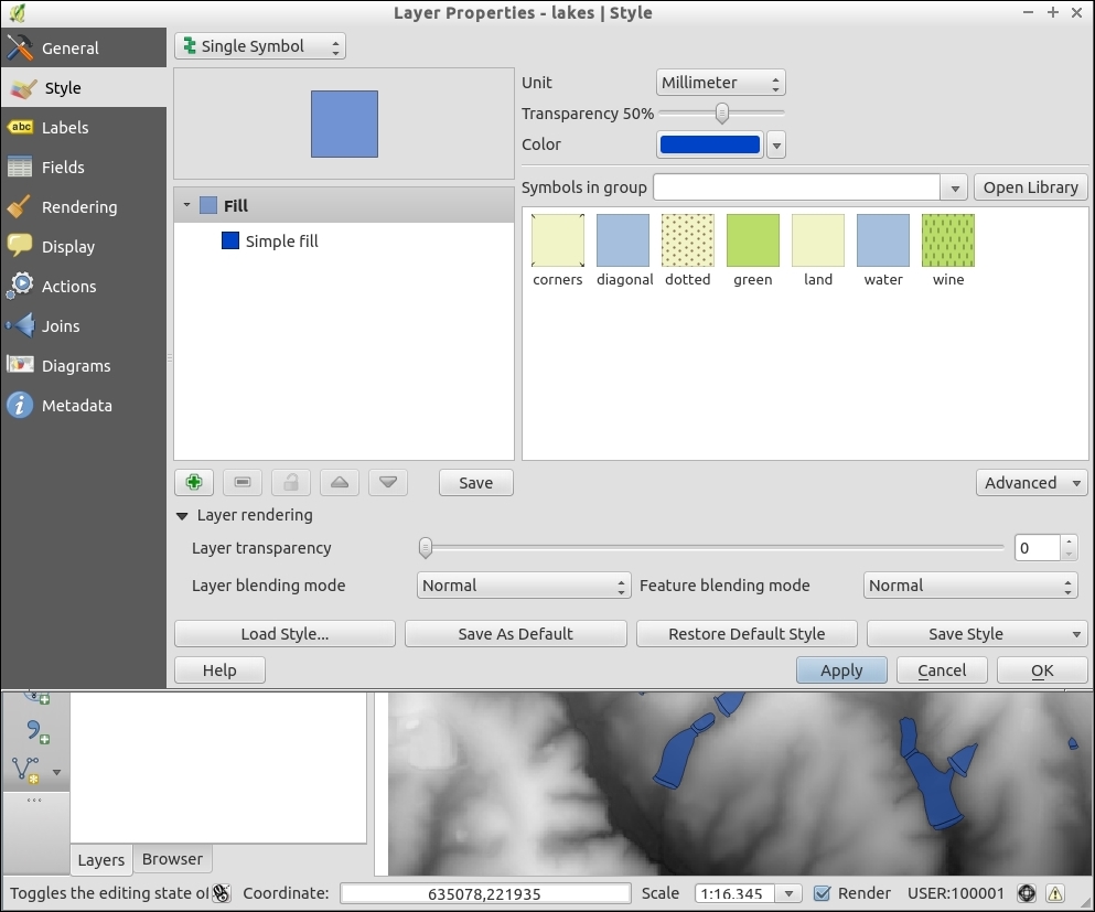
- With a vector layer loaded, open Properties and the Style tab.
- On the right-hand side of the dialog, you will see a Transparency slider at 0% (this means 100% solid or opaque).
- Adjust the slider to the right and apply the changes to see them in the map:
- Now to demonstrate this on a raster, first reset the lakes back to 0%.
- Swap the order in the Layers list so that
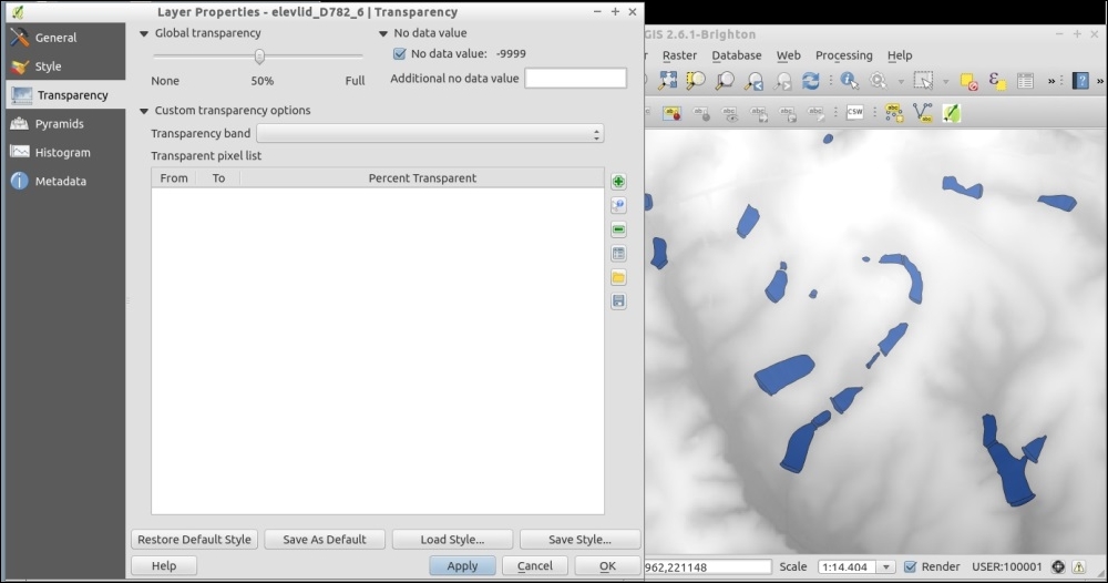
elevlidis on top. - Now, open Properties of
elevidand the Transparency tab. - The Global transparency option will change the value evenly for the whole raster. Set it to 50% and apply it. You should now be able to see the lakes layer, which was hidden below:
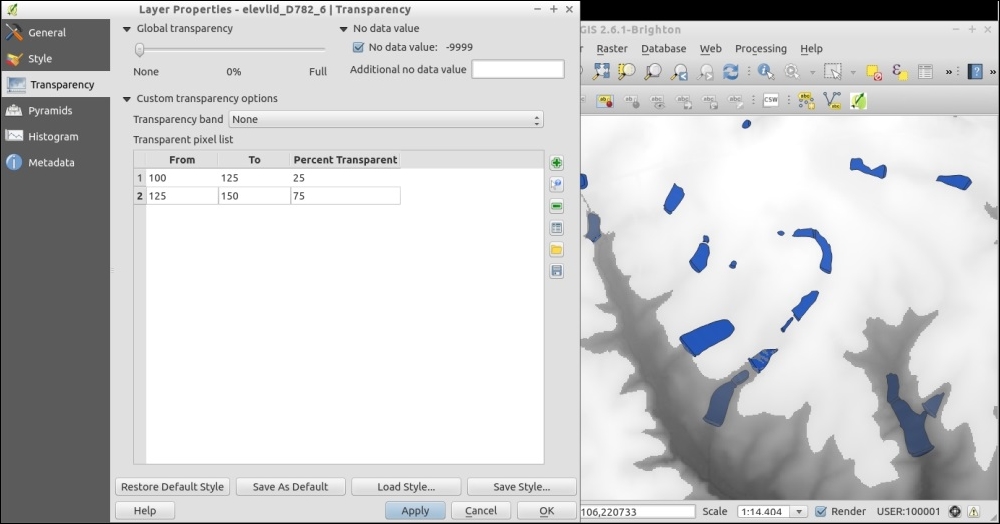
- (Optional) You may have noticed that below the Global transparency slider is Custom transparency options. This will allow you to make particular values more transparent than others. You can either assign specific values to specific transparencies, or you can add a band to the raster (or use a multiband raster), which specifies the amount of transparency to apply to the rest of the raster (some data formats, such as GeoTiff, call this an Alpha Transparency band):
- Reset the global back to 0% (otherwise, this is applied in too)
- Use the green + sign to add some values
- From 100 To 125, 25% transparent
- From 125 To 150, 75% transparent
- Click Apply and notice the lower elevation lakes are harder to see:
This is really a computer graphics thing, but the simplest explanation is that you're telling the computer to combine a percentage of two different layers in the same location instead of the top layer's value covering. Based on the math of the original colors and their transparency, a blended color is calculated for each pixel on the screen.
This doesn't begin to explain all the possible variations of appearance that can be achieved by mixing multiple layers and multiple transparencies, only tinkering can show you this.
One classic example of transparencies is to mix hillshades and airphotos. You can place either layer on top and then adjust the transparency to let the other show through. Generally, you would place the hillshade underneath in this case (but either can work). The end result is a landscape that appears to have 3D relief, but it looks like an airphoto.
Another classic example is to create a mask layer with a hole cut out around the region that you want to emphasize. You now place the mask layer on top. Before adding transparency, it blocks everything but the hole. Then, you slowly add transparency so that you can see surrounding regions, but they are muted and stand out less. For this technique, try a black, gray, or white fill for the mask layer. Each will have a slightly different look.
When styling vectors, you can apply different transparencies to different features in the same layer if you use Rule Based Rendering. Each rule can have a different transparency value and the entire layer can have yet another transparency modifier in the Layer Rendering section.
Lastly, keep in mind that not all output formats handle transparency well. In particular, be careful using color gradients with transparencies when exporting to PDF. Generally, PNG handles transparency, SVG may work or at least allow to you to edit the transparency after export, unlike image formats.