Editing vector geometries

Now that we know how to create and select features, we can take a closer look at the other tools in the Digitizing and Advanced Digitizing toolbars.

Using basic digitizing tools

This is the basic Digitizing toolbar:

The Digitizing toolbar contains tools that we can use to create and move features and nodes as well as delete, copy, cut, and paste features, as follows:

The Add Feature tool allows us to create new features by placing feature nodes on the map, which are connected by straight lines.
Similarly, the Add Circular String tool allows us to create features where consecutive nodes are connected by curved lines.
With the Move Feature(s) tool, it is easy to move one or more features at once by dragging them to the new location.
Similarly, the Node Tool feature allows us to move one or more nodes of the same feature. The first click activates the feature, while the second click selects the node. Hold the mouse key down to drag the node to its new location. Instead of moving only one node, we can also move an edge by clicking and dragging the line. Finally, we can select and move multiple nodes by holding down the Ctrl key.
The Delete Selected, Cut Features, and Copy Features tools are active only if one or more layer features are selected. Similarly, Paste Features works only after a feature has been cut or copied.

Using advanced digitizing tools

The Advanced Digitizing toolbar offers very useful Undo and Redo functionalities as well as additional tools for more involved geometry editing, as shown in the following screenshot:

The Advanced Digitizing tools include the following:

Rotate Feature(s) enables us to rotate one or more selected features around a central point.
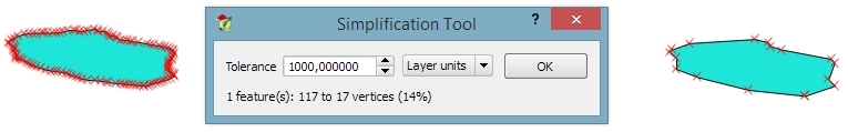
Using the Simplify Feature tool, we can simplify/generalize feature geometries by simply clicking on the feature and specifying a desired tolerance in the pop-up window, as shown in the following screenshot, where you can see the original geometry on the left-hand side and the simplified geometry on the right-hand side:
The following tools can be used to modify polygons. They allow us to add rings, also known as holes, into existing polygons or add parts to them. The Fill Ring tool is similar to Add Ring, but instead of just creating a hole, it also creates a new feature that fills the hole. Of course, there are tools to delete rings and parts well.
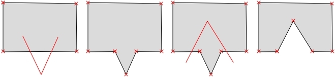
The Reshape Features tool can be used to alter the geometry of a feature by either cutting out or adding pieces. You can control the behavior by starting to draw the new form inside the original feature to add a piece, or by starting outside to cut out a piece, as shown in this example diagram:
The Offset Curve tool is only available for lines and allows us to displace a line geometry by a given offset.
The Split Features tool allows us to split one or more features into multiple features along a cut line. Similarly, Split Parts allows us to split a feature into multiple parts that still belong to the same multipolygon or multipolyline.
The Merge Selected Features tool enables us to merge multiple features while keeping control over which feature's attributes will be available in the output feature.
Similarly, Merge Attributes of Selected Features also lets us combine the attributes of multiple features but without merging them into one feature. Instead, all the original features remain as they were; the attribute values are updated.
Finally, Rotate Point Symbols is available only for point layers with the Rotation field feature enabled (we will cover this feature in Chapter 5, Creating Great Maps).

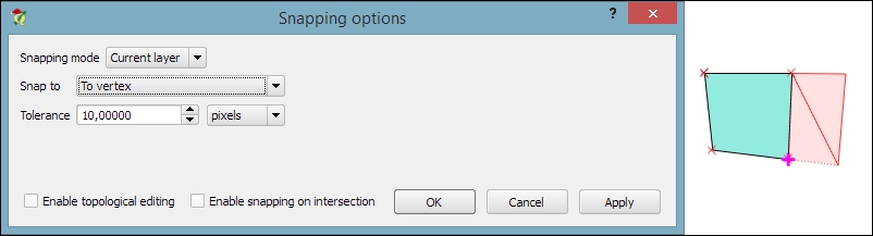
Using snapping to enable topologically correct editing

One of the challenges of digitizing features by hand is avoiding undesired gaps or overlapping features. To make it easier to avoid these issues, QGIS offers a snapping functionality. To configure snapping, we go to Settings | Snapping options. The following screenshot shows how to enable snapping for the Current layer. Similarly, you can choose snapping modes for All layers or the Advanced mode, where you can control the settings for each layer separately. In the example shown in the following screenshot, we enable snapping To vertex. This means that digitizing tools will automatically snap to vertices/nodes of existing features in the current layer. Similarly, you can enable snapping To segment or To vertex and segment. When snapping is enabled during digitizing, you will notice bold cross-shaped markers appearing whenever you go close to a vertex or segment that can be snapped to:

Previous Chapter

Working with feature selection tools

Next Chapter

Using measuring tools

Table of Contents for QGIS: Becoming a GIS Power User

Editing vector geometries

Using basic digitizing tools

Using advanced digitizing tools

Using snapping to enable topologically correct editing

Table of Contents for
QGIS: Becoming a GIS Power User