Table of Contents for
QGIS: Becoming a GIS Power User
 QGIS: Becoming a GIS Power User
Published by
Packt Publishing, 2017
QGIS: Becoming a GIS Power User
Published by
Packt Publishing, 2017
- Cover
- Table of Contents
- QGIS: Becoming a GIS Power User
- QGIS: Becoming a GIS Power User
- QGIS: Becoming a GIS Power User
- Credits
- Preface
- What you need for this learning path
- Who this learning path is for
- Reader feedback
- Customer support
- 1. Module 1
- 1. Getting Started with QGIS
- Running QGIS for the first time
- Introducing the QGIS user interface
- Finding help and reporting issues
- Summary
- 2. Viewing Spatial Data
- Dealing with coordinate reference systems
- Loading raster files
- Loading data from databases
- Loading data from OGC web services
- Styling raster layers
- Styling vector layers
- Loading background maps
- Dealing with project files
- Summary
- 3. Data Creation and Editing
- Working with feature selection tools
- Editing vector geometries
- Using measuring tools
- Editing attributes
- Reprojecting and converting vector and raster data
- Joining tabular data
- Using temporary scratch layers
- Checking for topological errors and fixing them
- Adding data to spatial databases
- Summary
- 4. Spatial Analysis
- Combining raster and vector data
- Vector and raster analysis with Processing
- Leveraging the power of spatial databases
- Summary
- 5. Creating Great Maps
- Labeling
- Designing print maps
- Presenting your maps online
- Summary
- 6. Extending QGIS with Python
- Getting to know the Python Console
- Creating custom geoprocessing scripts using Python
- Developing your first plugin
- Summary
- 2. Module 2
- 1. Exploring Places – from Concept to Interface
- Acquiring data for geospatial applications
- Visualizing GIS data
- The basemap
- Summary
- 2. Identifying the Best Places
- Raster analysis
- Publishing the results as a web application
- Summary
- 3. Discovering Physical Relationships
- Spatial join for a performant operational layer interaction
- The CartoDB platform
- Leaflet and an external API: CartoDB SQL
- Summary
- 4. Finding the Best Way to Get There
- OpenStreetMap data for topology
- Database importing and topological relationships
- Creating the travel time isochron polygons
- Generating the shortest paths for all students
- Web applications – creating safe corridors
- Summary
- 5. Demonstrating Change
- TopoJSON
- The D3 data visualization library
- Summary
- 6. Estimating Unknown Values
- Interpolated model values
- A dynamic web application – OpenLayers AJAX with Python and SpatiaLite
- Summary
- 7. Mapping for Enterprises and Communities
- The cartographic rendering of geospatial data – MBTiles and UTFGrid
- Interacting with Mapbox services
- Putting it all together
- Going further – local MBTiles hosting with TileStream
- Summary
- 3. Module 3
- 1. Data Input and Output
- Finding geospatial data on your computer
- Describing data sources
- Importing data from text files
- Importing KML/KMZ files
- Importing DXF/DWG files
- Opening a NetCDF file
- Saving a vector layer
- Saving a raster layer
- Reprojecting a layer
- Batch format conversion
- Batch reprojection
- Loading vector layers into SpatiaLite
- Loading vector layers into PostGIS
- 2. Data Management
- Joining layer data
- Cleaning up the attribute table
- Configuring relations
- Joining tables in databases
- Creating views in SpatiaLite
- Creating views in PostGIS
- Creating spatial indexes
- Georeferencing rasters
- Georeferencing vector layers
- Creating raster overviews (pyramids)
- Building virtual rasters (catalogs)
- 3. Common Data Preprocessing Steps
- Converting points to lines to polygons and back – QGIS
- Converting points to lines to polygons and back – SpatiaLite
- Converting points to lines to polygons and back – PostGIS
- Cropping rasters
- Clipping vectors
- Extracting vectors
- Converting rasters to vectors
- Converting vectors to rasters
- Building DateTime strings
- Geotagging photos
- 4. Data Exploration
- Listing unique values in a column
- Exploring numeric value distribution in a column
- Exploring spatiotemporal vector data using Time Manager
- Creating animations using Time Manager
- Designing time-dependent styles
- Loading BaseMaps with the QuickMapServices plugin
- Loading BaseMaps with the OpenLayers plugin
- Viewing geotagged photos
- 5. Classic Vector Analysis
- Selecting optimum sites
- Dasymetric mapping
- Calculating regional statistics
- Estimating density heatmaps
- Estimating values based on samples
- 6. Network Analysis
- Creating a simple routing network
- Calculating the shortest paths using the Road graph plugin
- Routing with one-way streets in the Road graph plugin
- Calculating the shortest paths with the QGIS network analysis library
- Routing point sequences
- Automating multiple route computation using batch processing
- Matching points to the nearest line
- Creating a routing network for pgRouting
- Visualizing the pgRouting results in QGIS
- Using the pgRoutingLayer plugin for convenience
- Getting network data from the OSM
- 7. Raster Analysis I
- Using the raster calculator
- Preparing elevation data
- Calculating a slope
- Calculating a hillshade layer
- Analyzing hydrology
- Calculating a topographic index
- Automating analysis tasks using the graphical modeler
- 8. Raster Analysis II
- Calculating NDVI
- Handling null values
- Setting extents with masks
- Sampling a raster layer
- Visualizing multispectral layers
- Modifying and reclassifying values in raster layers
- Performing supervised classification of raster layers
- 9. QGIS and the Web
- Using web services
- Using WFS and WFS-T
- Searching CSW
- Using WMS and WMS Tiles
- Using WCS
- Using GDAL
- Serving web maps with the QGIS server
- Scale-dependent rendering
- Hooking up web clients
- Managing GeoServer from QGIS
- 10. Cartography Tips
- Using Rule Based Rendering
- Handling transparencies
- Understanding the feature and layer blending modes
- Saving and loading styles
- Configuring data-defined labels
- Creating custom SVG graphics
- Making pretty graticules in any projection
- Making useful graticules in printed maps
- Creating a map series using Atlas
- 11. Extending QGIS
- Defining custom projections
- Working near the dateline
- Working offline
- Using the QspatiaLite plugin
- Adding plugins with Python dependencies
- Using the Python console
- Writing Processing algorithms
- Writing QGIS plugins
- Using external tools
- 12. Up and Coming
- Preparing LiDAR data
- Opening File Geodatabases with the OpenFileGDB driver
- Using Geopackages
- The PostGIS Topology Editor plugin
- The Topology Checker plugin
- GRASS Topology tools
- Hunting for bugs
- Reporting bugs
- Bibliography
- Index
Optimum site selection is a pretty common problem, for example, when planning shop or warehouse locations or when looking for a new apartment. In this recipe, you will learn how to perform optimum site selection manually using tools from the Processing Toolbox option, but you will also see how to automate this workflow by creating a Processing model.
In the optimum site selection in this recipe, we will combine different vector analysis tools to find potential locations in Wake County that match the following criteria:
- Locations are near a big lake (up to 500 m)
- Locations are close to an elementary school (up to 500 m)
- Locations are within a reasonable distance (up to 2 km) from a high school
- Locations are at least 1 km from a main road
To follow this exercise, load the following datasets, lakes.shp, schools_wake.shp, and roadsmajor.shp.
As all datasets in our test data already use the same CRS, we can get right to the analysis. If you are using different data, you may have to get all your datasets into the same CRS first. In this case, please refer to Chapter 1, Data Input and Output.
The following steps show you how to perform optimum site selection using the Processing Toolbox option:
- First, we have to filter the lakes layer for big lakes. To do this, we use the Select by expression tool from the Processing toolbox, select the lakes layer, and enter
"AREA" > 1000000 AND "FTYPE" = 'LAKE/POND'in the Expression textbox, as shown in the following screenshot: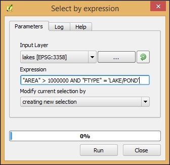
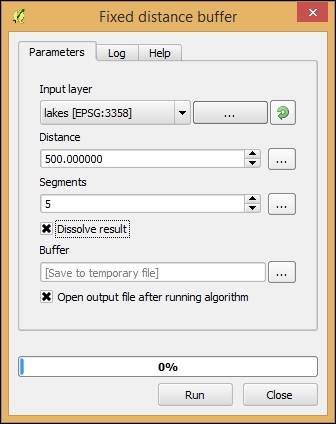
- Next, we create the buffers that will represent the proximity areas around lakes, schools, and roads. Use Fixed distance buffer from the Processing Toolbox option to create the following buffers:
- For the lakes, select Distance of 500 meters and set Dissolve result by checking the box as shown in the following screenshot. By dissolving the result, we can make sure that the overlapping buffer areas will be combined into one polygon. Otherwise, each buffer will remain as a separate feature in the resulting layer:
- To create the elementary school buffers, first select only the schools with
"GLEVEL" = 'E'using the Select by Expression tool like we did for the lakes buffer. Then, use the buffer tool like we just did for the lakes buffer. - Repeat the process for the high schools using
"GLEVEL" = 'H'and a buffer distance of 2,000 meters. - Finally, for the roads, create a buffer with a distance of 1,000 meters.
- For the lakes, select Distance of 500 meters and set Dissolve result by checking the box as shown in the following screenshot. By dissolving the result, we can make sure that the overlapping buffer areas will be combined into one polygon. Otherwise, each buffer will remain as a separate feature in the resulting layer:
- With all these buffers ready, we can now combine them to fulfill these rules:
- Use the Intersection tool from the Processing Toolbox option on the buffers around elementary and high schools to get the areas that are within the vicinity of both school types.
- Use the Intersection tool on the buffers around the lakes and the result of the previous step to limit the results to lakeside areas. Use the Difference tool to remove areas around major roads (that is, the buffered road layer) from the result of the previous (Intersection) steps.
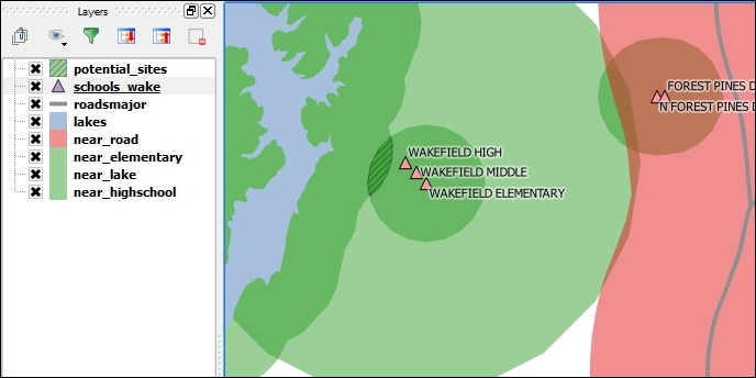
- Check the resulting layer to view the potential sites that fit all the criteria that we previously specified. You'll find that there is only one area close to WAKEFIELD ELEMENTARY and WAKEFIELD HIGH that fits the bill, as shown in the following screenshot:
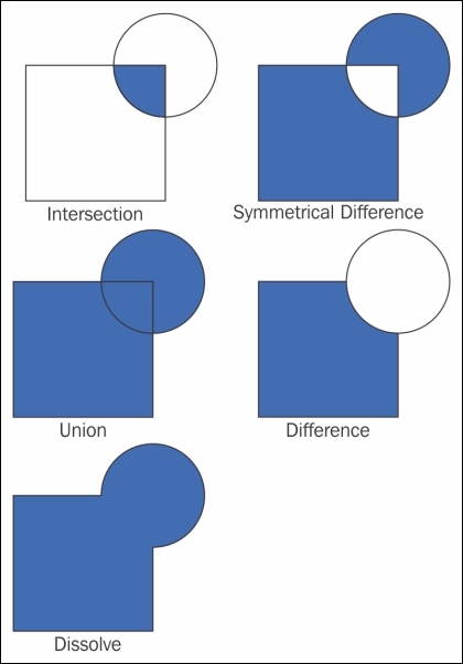
In step 1, we used Intersection to model the requirement that our preferred site would be near both an elementary and a high school. Later, in step 3, the Difference tool enabled us to remove areas close to major roads. The following figure gives us an overview of the available vector analysis tools that can be useful for similar analyses. For example, Union could be used to model requirements, such as "close to at least an elementary or a high school". Symmetrical Difference, on the other hand, would result in "close to an elementary or a high school but not both", as illustrated in the following figure:
We were lucky and found a potential site that matched all criteria. Of course, this is not always the case, and you will have to try and adjust your criteria to find a matching site. As you can imagine, it can be very tedious and time-consuming to repeat these steps again and again with different settings. Therefore, it's a good idea to create a Processing model to automate this task.
The model (as shown in the following screenshot) basically contains the same tools that we used in the manual process, as follows:
- Use two select by expression instances to select elementary and high schools. As you can see in the following screenshot, we used the descriptions Select "GLEVEL" = 'E' and Select "GLEVEL" = 'H' to name these model steps.
- For elementary schools, compute fixed distance buffers of 500 meters. This step is called Buffer "GLEVEL" = 'E'.
- For high schools, compute fixed distance buffers of 2,000 meters. This step is called Buffer "GLEVEL" = 'H'.
- Select the big lakes using
Select byexpression (refer to the Select big lakes step) and buffer them using fixed distance buffer of 500 meters (refer to the Buffer lakes step). - Buffer the roads using Fixed distance buffer (refer to the Buffer roads step). The buffer size is controlled by the number model input called road_buffer_size. You can extend this approach of controlling the model parameters using additional inputs to all the other buffer steps in this model. (We chose to show only one example in order to keep the model screenshot readable.)
- Use Intersection to get areas near schools (refer to the Intersection: near schools step).
- Use Intersection to get areas near schools and lakes (refer to the Intersection: schools and lakes step).
- Use Difference to remove areas near roads (refer to the Difference: avoid roads step).
This is how the final model looks like:
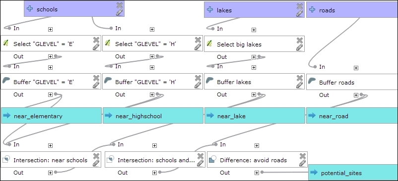
You can run this model from the Processing Toolbox option, or you can even use it as a building block in other models. It is worth noting that this model produces intermediate results in the form of buffer results (near_elementary, near highschool, and so on). While these intermediate results are useful while developing and debugging the model, you may eventually want to remove them. This can be done by editing the buffer steps and removing the Buffer <OutputVector> names.