The cartographic rendering of geospatial data – MBTiles and UTFGrid

At this point, you may be wondering, what about the maps? So far, we have not included any geospatial data or visualization. We will be offloading some of the effort in managing and providing geospatial data and services to OpenStreetMap—our favorite public open source geospatial data repository!

Note

Why do we use OpenStreetMap?

OSM already provides mirrored map services for quick reproduction in the basemaps
OSM provides a very extensive and scalable schema for the kind of geographic features that you might find on a campus
Various web, mobile, and desktop clients have already been written to interact with the OSM API
OSM provides the databases and other infrastructure, so we don't have to
OSM has a granular and reliable way to track changes, using the osm_version and osm_user fields, which complement the osm_id unique ID field

OpenStreetMap to SpatiaLite

To use the OSM data, we need to get it in a format that will be interoperable with other GIS software components. A quick and powerful solution is to store the OSM data in a SQLite SpatiaLite database instance, which, if you remember, is a single file with full spatial and SQL functionality.

To use QGIS to download and convert OSM to SQLite, perform the following steps:

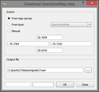
Obtain the OSM data in the same way that we did in Chapter 4, Finding the Best Way to Get There. Use the OpenLayers plugin to zoom into Newark, DE (or use the extent, 39.7009, -75.7195, 39.6542, -75.7784, clockwise from the top of the dialog in the next step):
1. Navigate to Vector | OpenStreetMap | Download Data to download the OSM data for this extent.
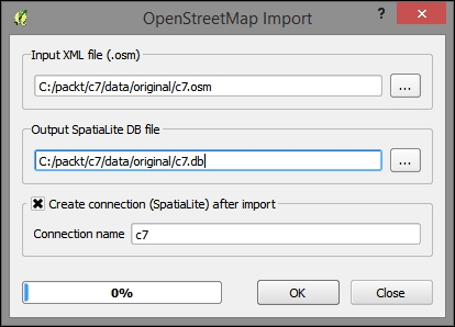
Next, export the XML data in the .osm file to a topological SQLite database. This could potentially be used for routing; although, we will not be doing so here.
1. Navigate to Vector | OpenStreetMap | Import Topology from XML.
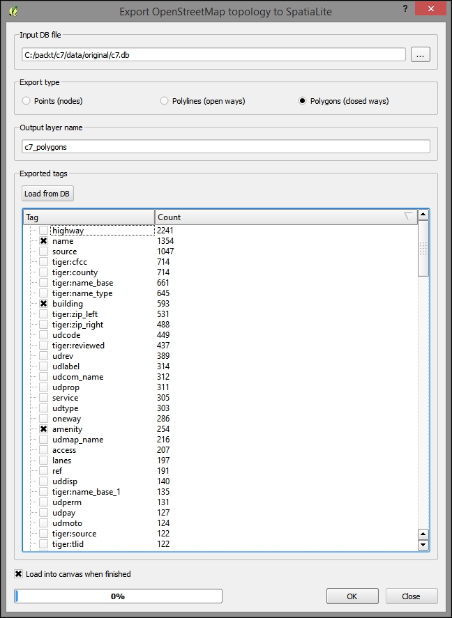
Next, export the topological data to normal geospatial data—polygons in this case.
1. Navigate to Vector | OpenStreetMap | Export topology to SpatiaLite.
2. Export type: Polygons (closed ways).
3. Click on Load from DB to populate the list of fields in the data. Select the fields amenity, building, name, and leisure, as shown in the following screenshot, as fit allowed:
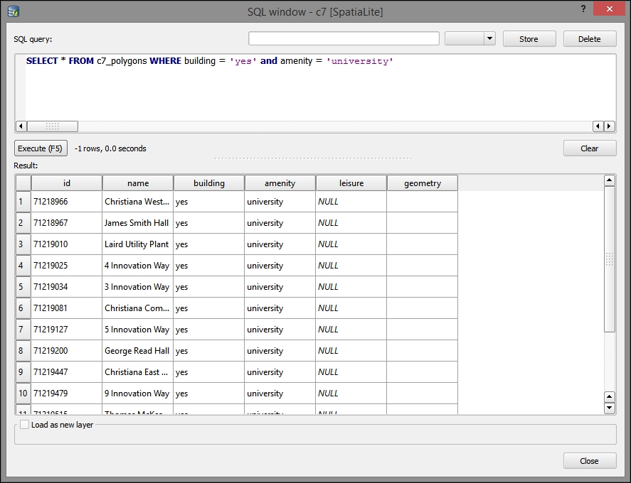
Use DB Manager to display the university buildings.
1. Navigate to Database | DB Manager | DB Manager.
2. Highlight the c7 SQLite database.
3. Execute the following query, ensuring that Load as new layer is selected:
```
SELECT * FROM c7_polygons WHERE building = 'yes' and amenity = 'university'
```
Export the query layer to c7/data/original/delaware-latest-3875/buildings.shp with the EPSG:3857 projection.

To tile and use UTFGrid with TileMill

Although TileMill is no longer under active production by its creator Mapbox, it is still useful for us to produce MBTiles tiled images rendered by Mapnik using CartoCSS and a UTFGrid interaction layer.

Preparing a basemap from OSM

TileMill requires that all the data be rendered and tiled together and, therefore, only supports vector data input, including JSON, shapefile, SpatiaLite, and PostGIS.

In the following steps, we will render a cartographically pleasing map as a .mbtiles (single-file-based) tile cache:

Install and open TileMill.
Download the Delaware data from the North America section of the Geofabrik OSM extracts site (http://download.geofabrik.de/north-america.html) as a shapefile. Alternatively, you can directly download it from http://download.geofabrik.de/north-america/us/delaware-latest.shp.zip. Ensure that you expand and copy the zip archive to your project directory after you've downloaded it.
Reproject all the data from EPSG:4326 to :3875. If you remember, QGIS can do this in batch as with other Processing Toolbox algorithms, as you learned in Chapter 2, Identifying the Best Places, making this process a bit quicker.
Output all the layers to c7/data/original/delaware-latest-3875.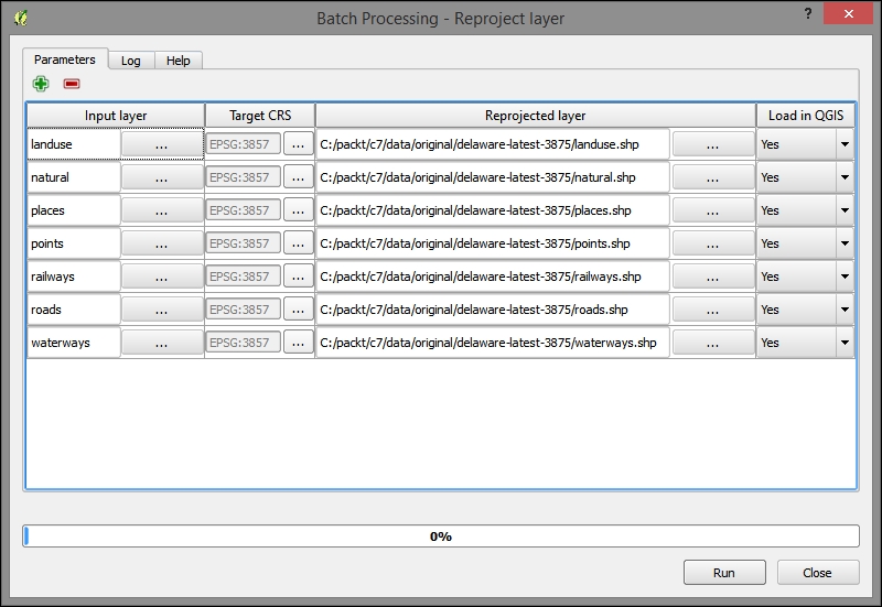
Copy the DC example to a new project.
- You will find it in C:\Program Files (x86)\TileMill-v0.10.1\tilemill\examples\open-streets-dc
- Copy it to C:\Users\[YOURUSERNAME]\Documents\MapBox\project\c7
Delete all the files from the layers directory.
Copy and extract all the shapefiles from c7/data/original/delaware-latest-3875 into the layers directory in the project directory of c7, which can be found at C:\Users\[YOURUSERNAME]\Documents\MapBox\project\c7\layers.
Edit the project.mml file.
1. Change all the instances of the open-streets-dc string to c7.
2. Change the single instance of Open Streets, DC to c7.
3. Substitute the following bounds and center:
```
  "bounds": [
    -75.7845,
    39.6586,
    -75.7187,
    39.71
  ],
  "center": [
    -75.7538,
    39.6827,
    14
],
```
4. Change the following layer references to files:
  Land usages: Change this layer from osm-landusages.shp to landuse.shp
  ocean: Remove this layer or ignore
  water: Change this layer from osm-waterareas.shp to waterways.shp
  tunnels: Change this layer from osm-roads.shp to roads.shp
  roads: Change this layer from osm-roads.shp to roads.shp
  mainroads: Change this layer from osm-mainroads.shp to roads.shp
  motorways: Change this layer from osm-motorways.shp to roads.shp
  bridges: Change this layer from osm-roads.shp to roads.shp
  places: Change this layer from osm-places.shp to places.shp
  road-label: Change this layer from osm-roads.shp to roads.shp
Open TileMill and select the c7 project from the Projects dialog, as shown in the following screenshot: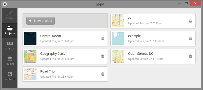

Preparing the operational layer in TileMill

Open the Layers panel from the bottommost button in the bottom-left corner. Refer to the next image.
Click on + Add layer.
Populate the parameters with the following values:
- ID: buildings.
- Datasource: c7/data/original/delaware-latest-3875/buildings.shp.
- Click on Save & Style. You can return to this dialog later by clicking on the Editor button (pencil icon) in the Layers panel, by the #c7 layer, as shown in the next image.
If you don't yet see your layer, ensure that you have some style defined in the tab on the right that will be applied to the layer (this should be populated by default with a minimal style). Then, click on Save in the top-right corner.
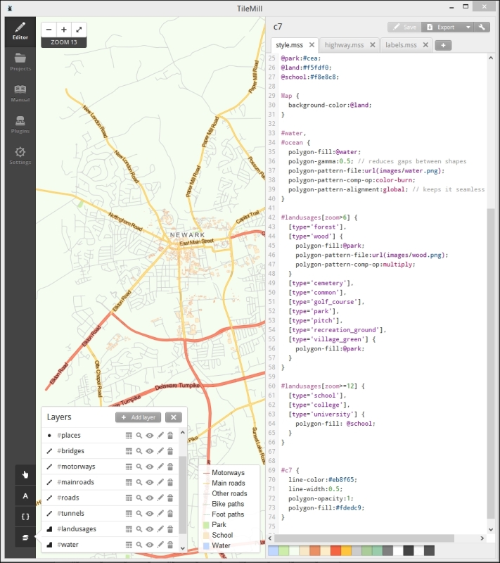
Use the CartoCSS syntax to change the style in style.mss. TileMill provides a color picker, which we can access by clicking on a swatch color at the bottom of the CartoCSS/style pane. After changing a color, you can view the hex code down there. Just pick a color, place the hex code in your CartoCSS, and save it. For example, consider the following code:
```
#buildings {
  line-color:#eb8f65;
  line-width:0.5;
  polygon-opacity:1;
  polygon-fill:#fdedc9;
}
```
Click on Save (with the pencil icon) in the upper-right corner of the main screen (above the CartoCSS input) to view the changes, as shown in the following screenshot:
Go to the Templates tab by clicking on the topmost button in the lower-left corner and change the Teaser and Full interaction types to use {{{id}}} from buildings, as shown in the following screenshot: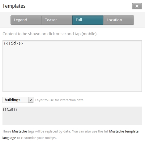

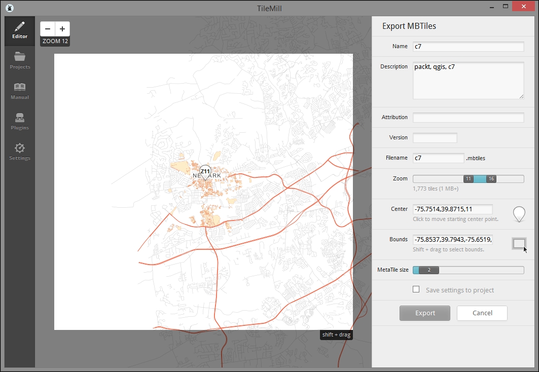
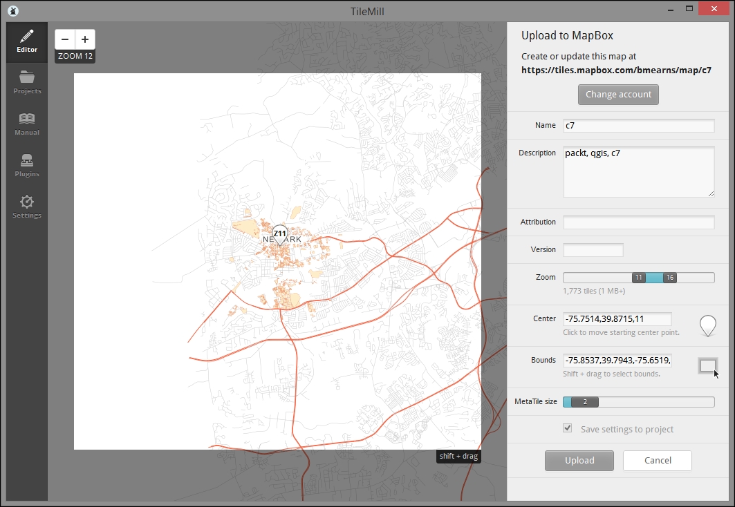
Exporting MBTiles

MBTiles is a format developed by Mapbox to store geographic information. There are two compelling aspects of this format, besides interaction with a small but impressive suite of software and services developed by Mapbox: firstly, MBTiles stores a whole tile store in a single file, which is easy to transfer and maintain and secondly, UTFGrid, which is the use of UTF characters for highly performant data interaction, is enabled by this format.

Uploading to Mapbox

Perform the following steps:

Create an account on mapbox.com.
Access the Export dialog from the Export button in the upper-right corner. Select Upload from this menu.
Sign in to your Mapbox account by clicking on the button at the top of the dialog.
Press Shift, click on it, and drag to define an extent in the map.
Zoom to one level above your intended minimum zoom to preview the extent.
Fill in the descriptive information in the export dialog.
- Name: c7
- Zoom: 11 to 16
Click on the map to establish a Center coordinate.
Select Save settings to project.
Upload, as shown in the following screenshot:

The MBTiles file

The steps for exporting directly to an MBTiles file are similar to the previous procedure. This format can be uploaded to mapbox.com or served with software that supports the format, such as TileStream. Of course, no sign-on is needed.

Previous Chapter

7. Mapping for Enterprises and Communities

Next Chapter

Interacting with Mapbox services

Table of Contents for QGIS: Becoming a GIS Power User