You'll need a raster file that you want to cut a portion of. In this example, we will use the North Carolina whole state elevation model (elev_state_500m.tif) and cut it with the outline of Wake County (county_wake.shp). Load both of these files in a fresh QGIS project.

The easiest way to do this is to use a polygon mask layer. The vector mask can be a rectangle, but it doesn't have to be. The outline of a single polygon works best, though.

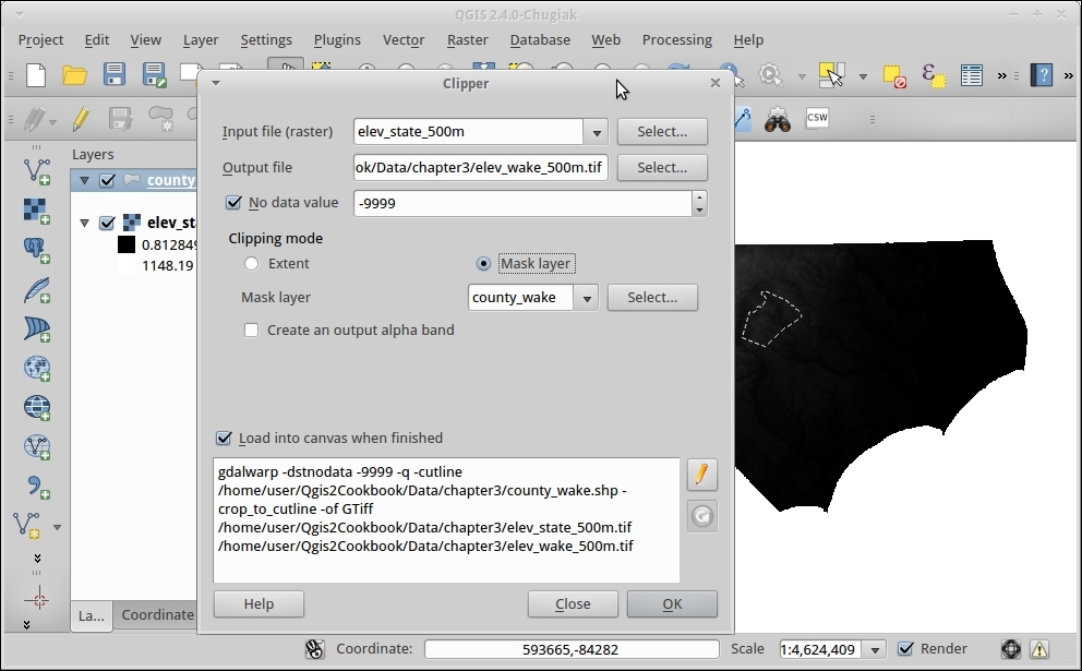
The shape of your mask and the size of the raster cells in the source data will determine how pixelated the resulting raster will be. Zoom in to the results and compare the edge of the new raster to the vector outline of the county. You'll notice that because of the 500 m wide pixels, it's hard to exactly match the edge of the county exactly with whole pixels.

Note that this tool, as with all other tools in the GDAL Tools menu, is actually a graphical interface to GDAL command-line tools.

You'll notice that with this particular example, an issue that arises with converting rasters to nonrectangular shapes; the edges are jagged as compared to the vector. If you need it to be really smooth, there are a few options. You can decrease the pixel size, splitting current pixels into multiple pixels using the -tr option. As with other Raster tools, you can use the pencil icon to override the GDAL command-line options to add features not included in the interface. In this case, the -tr option inline with the rest of the already formatted command:

gdalwarp -tr 100 100

This would make each pixel 100 units instead of the current 500 x 500.