Table of Contents for
QGIS: Becoming a GIS Power User
 QGIS: Becoming a GIS Power User
Published by
Packt Publishing, 2017
QGIS: Becoming a GIS Power User
Published by
Packt Publishing, 2017
- Cover
- Table of Contents
- QGIS: Becoming a GIS Power User
- QGIS: Becoming a GIS Power User
- QGIS: Becoming a GIS Power User
- Credits
- Preface
- What you need for this learning path
- Who this learning path is for
- Reader feedback
- Customer support
- 1. Module 1
- 1. Getting Started with QGIS
- Running QGIS for the first time
- Introducing the QGIS user interface
- Finding help and reporting issues
- Summary
- 2. Viewing Spatial Data
- Dealing with coordinate reference systems
- Loading raster files
- Loading data from databases
- Loading data from OGC web services
- Styling raster layers
- Styling vector layers
- Loading background maps
- Dealing with project files
- Summary
- 3. Data Creation and Editing
- Working with feature selection tools
- Editing vector geometries
- Using measuring tools
- Editing attributes
- Reprojecting and converting vector and raster data
- Joining tabular data
- Using temporary scratch layers
- Checking for topological errors and fixing them
- Adding data to spatial databases
- Summary
- 4. Spatial Analysis
- Combining raster and vector data
- Vector and raster analysis with Processing
- Leveraging the power of spatial databases
- Summary
- 5. Creating Great Maps
- Labeling
- Designing print maps
- Presenting your maps online
- Summary
- 6. Extending QGIS with Python
- Getting to know the Python Console
- Creating custom geoprocessing scripts using Python
- Developing your first plugin
- Summary
- 2. Module 2
- 1. Exploring Places – from Concept to Interface
- Acquiring data for geospatial applications
- Visualizing GIS data
- The basemap
- Summary
- 2. Identifying the Best Places
- Raster analysis
- Publishing the results as a web application
- Summary
- 3. Discovering Physical Relationships
- Spatial join for a performant operational layer interaction
- The CartoDB platform
- Leaflet and an external API: CartoDB SQL
- Summary
- 4. Finding the Best Way to Get There
- OpenStreetMap data for topology
- Database importing and topological relationships
- Creating the travel time isochron polygons
- Generating the shortest paths for all students
- Web applications – creating safe corridors
- Summary
- 5. Demonstrating Change
- TopoJSON
- The D3 data visualization library
- Summary
- 6. Estimating Unknown Values
- Interpolated model values
- A dynamic web application – OpenLayers AJAX with Python and SpatiaLite
- Summary
- 7. Mapping for Enterprises and Communities
- The cartographic rendering of geospatial data – MBTiles and UTFGrid
- Interacting with Mapbox services
- Putting it all together
- Going further – local MBTiles hosting with TileStream
- Summary
- 3. Module 3
- 1. Data Input and Output
- Finding geospatial data on your computer
- Describing data sources
- Importing data from text files
- Importing KML/KMZ files
- Importing DXF/DWG files
- Opening a NetCDF file
- Saving a vector layer
- Saving a raster layer
- Reprojecting a layer
- Batch format conversion
- Batch reprojection
- Loading vector layers into SpatiaLite
- Loading vector layers into PostGIS
- 2. Data Management
- Joining layer data
- Cleaning up the attribute table
- Configuring relations
- Joining tables in databases
- Creating views in SpatiaLite
- Creating views in PostGIS
- Creating spatial indexes
- Georeferencing rasters
- Georeferencing vector layers
- Creating raster overviews (pyramids)
- Building virtual rasters (catalogs)
- 3. Common Data Preprocessing Steps
- Converting points to lines to polygons and back – QGIS
- Converting points to lines to polygons and back – SpatiaLite
- Converting points to lines to polygons and back – PostGIS
- Cropping rasters
- Clipping vectors
- Extracting vectors
- Converting rasters to vectors
- Converting vectors to rasters
- Building DateTime strings
- Geotagging photos
- 4. Data Exploration
- Listing unique values in a column
- Exploring numeric value distribution in a column
- Exploring spatiotemporal vector data using Time Manager
- Creating animations using Time Manager
- Designing time-dependent styles
- Loading BaseMaps with the QuickMapServices plugin
- Loading BaseMaps with the OpenLayers plugin
- Viewing geotagged photos
- 5. Classic Vector Analysis
- Selecting optimum sites
- Dasymetric mapping
- Calculating regional statistics
- Estimating density heatmaps
- Estimating values based on samples
- 6. Network Analysis
- Creating a simple routing network
- Calculating the shortest paths using the Road graph plugin
- Routing with one-way streets in the Road graph plugin
- Calculating the shortest paths with the QGIS network analysis library
- Routing point sequences
- Automating multiple route computation using batch processing
- Matching points to the nearest line
- Creating a routing network for pgRouting
- Visualizing the pgRouting results in QGIS
- Using the pgRoutingLayer plugin for convenience
- Getting network data from the OSM
- 7. Raster Analysis I
- Using the raster calculator
- Preparing elevation data
- Calculating a slope
- Calculating a hillshade layer
- Analyzing hydrology
- Calculating a topographic index
- Automating analysis tasks using the graphical modeler
- 8. Raster Analysis II
- Calculating NDVI
- Handling null values
- Setting extents with masks
- Sampling a raster layer
- Visualizing multispectral layers
- Modifying and reclassifying values in raster layers
- Performing supervised classification of raster layers
- 9. QGIS and the Web
- Using web services
- Using WFS and WFS-T
- Searching CSW
- Using WMS and WMS Tiles
- Using WCS
- Using GDAL
- Serving web maps with the QGIS server
- Scale-dependent rendering
- Hooking up web clients
- Managing GeoServer from QGIS
- 10. Cartography Tips
- Using Rule Based Rendering
- Handling transparencies
- Understanding the feature and layer blending modes
- Saving and loading styles
- Configuring data-defined labels
- Creating custom SVG graphics
- Making pretty graticules in any projection
- Making useful graticules in printed maps
- Creating a map series using Atlas
- 11. Extending QGIS
- Defining custom projections
- Working near the dateline
- Working offline
- Using the QspatiaLite plugin
- Adding plugins with Python dependencies
- Using the Python console
- Writing Processing algorithms
- Writing QGIS plugins
- Using external tools
- 12. Up and Coming
- Preparing LiDAR data
- Opening File Geodatabases with the OpenFileGDB driver
- Using Geopackages
- The PostGIS Topology Editor plugin
- The Topology Checker plugin
- GRASS Topology tools
- Hunting for bugs
- Reporting bugs
- Bibliography
- Index
Dasymetric mapping is a technique that is commonly used to improve population distribution maps. By default, population is displayed using census data, which is usually available for geographic units, such as census tracts whose boundaries don't necessarily reflect the actual distribution of the population. To be able to model population distribution better, Dasymetric mapping enables us to map population density relative to land use. For example, population counts that are organized by census tracts can be more accurately distributed by removing unpopulated areas, such as water bodies or vacant land, from the census tract areas.
In this recipe, we will use data about populated urban areas, as well as data about water bodies to refine our census tract population data.
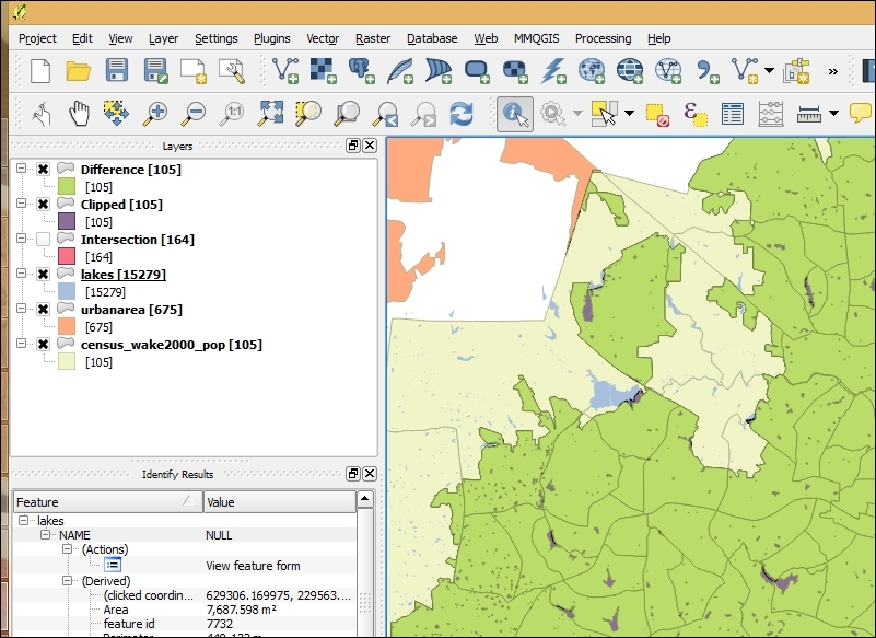
To follow this exercise, please load the population data from census_wake2000_pop.shp (the file that we created in Chapter 2, Data Management), as well as the urban areas from urbanarea.shp, and the lakes from lakes.shp.
As all the datasets in our sample data already use the same CRS, we can get right into the analysis. If you are using different data, you may have to first get all datasets into the same CRS. In this case, please refer to Chapter 1, Data Input and Output, for details.
To create a new and improved population distribution map, we will first remove the unpopulated areas from the census tracts. Then, we will recalculate the population density values to reflect the changes to the area geometries by performing the following steps:
- Use Clip from the Processing Toolbox option (or Clip by navigating to Vector | Geoprocessing tools if you prefer this option—the results will be identical) on the census tracts and urban area layers to create a new dataset, containing only those parts of the census tracts that are within urban areas.
- Refine the results of the previous step further by removing the water bodies (the lakes layer) using the Difference tool. The following screenshot shows the results of this so far:
- Now, we can calculate the population density of the resulting areas, as follows:
- Enable editing.
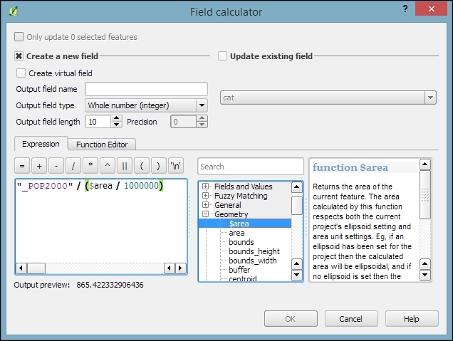
- Open Field calculator.
- Calculate a new population density (inhabitants per square km) using the formula, "_POP2000" / ($area / 1000000):
- Deactivate editing and save the changes.
Tip
It is worth noting that you don't necessarily have to make a new column. If you only want to use the density values for styling purposes, you can also enter the expression directly in the style configuration. On the other hand, if you create a new column, you can inspect the density values in the attribute table, export them, or analyze them further.
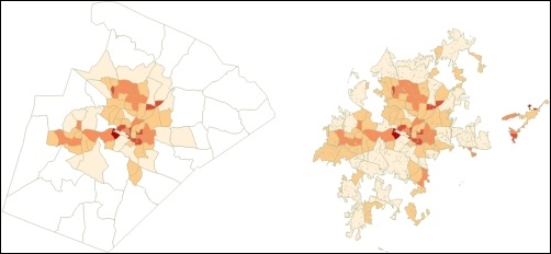
We are done, and you can now visualize the results using a Graduated renderer with, for example, the Natural Breaks (Jenks) classification mode. The Jenks Natural Breaks classification is designed to arrange values into "natural" classes by maximizing the variance between different classes while reducing the variance within the generated classes. The following figure shows the population density based on the original census data (on the left) and the results after Dasymetric mapping (on the right):
In the first step of this recipe, we used the Clip operation. As you most likely noticed, the results of a Clip operation look very similar to the results of the Intersection tool, which we used in the previous recipe of this chapter, Selecting optimum sites. Compare both the results, and you will see the following differences:
- The layer resulting from an Intersection operation contains attributes from both input layers, while the result of a Clip operation only contains attributes of the first input layer.
- This also means that the layer order is important when using Clip, but this does not change the output of Intersection (except for the attribute order in the attribute table).
- The Intersection result is also very likely to contain more features than the Clip result (164 instead of 105 if you use our sample data census tracts and urban areas). This is because the Intersect tool needs to create a new feature for every combination of intersecting census tracts and urban areas, while the Clip tool only removes the parts of the census tracts that are not within any urban area.
A popular way of thinking about the Clip operation is to imagine one layer as the cookie cutter and the other layer as the cookie dough.