Creating the travel time isochron polygons

Let's say that the school in our study is located at the vertex with an ID of 1 in the newark_osm layer. To visualize the walking time from the students' homes, without releasing sensitive information about where the students actually live, we can create isochron polygons. Each polygon will cover the area that a person can walk from to a single destination within some time threshold.

Generating the travel time for each road segment

We'll use DB Manager to create and populate a column for the travel time on each segment at the walking speed; then, we will create a query layer that includes the travel time from each road segment to our school at vertex 1. Perform the following steps:

Navigate to Database | DB Manager | DB Manager.
Select the database to be updated.
Go to Database | SQL window.

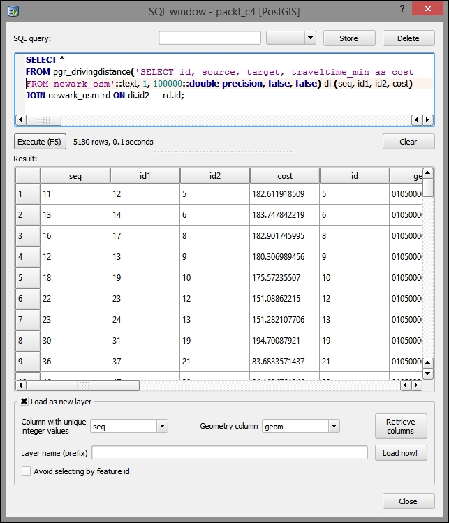
Enter the following code:

ALTER TABLE newark_osm ADD COLUMN traveltime_min float8;
UPDATE newark_osm SET traveltime_min = length_m  / 6000.0 * 60;

SELECT *
FROM pgr_drivingdistance('SELECT id, source, target, traveltime_min as cost FROM newark_osm'::text, 1, 100000::double precision, false, false) di (seq, id1, id2, cost)
JOIN newark_osm rd ON di.id2 = rd.id;

Select the Load as new layer option.
Select Retrieve columns.
Select seq as your Column with unique integer values and geom as your Geometry column.
Click on the Load now! button, as shown in the following screenshot:

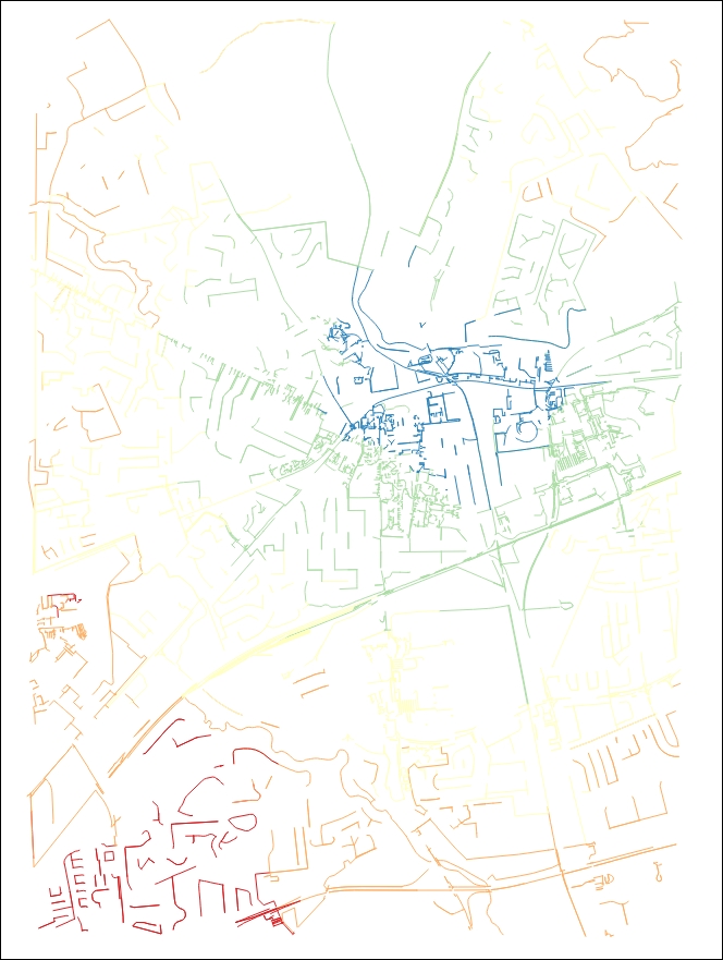
You can now symbolize the segments by the time it takes to get from that location to the school. To do this, use a Graduated style type with the traveltime_min field. You will see that the network segments with lower values (indicating quicker travel) are closer to vertex 1, and the opposite is true for the network segments with higher values. This method is limited by the extent to which the network models real conditions; for example, railroads are visualized along with other road segments for the travel time. However, railroads could cause discontinuity in our network—as they are not "traversable" by students traveling to school.

Generating the travel time for each road segment

Creating isochron polygons

Next, we will create the polygons to visualize the areas from which the students can walk to school in certain time ranges. We can use this technique to characterize the general travel time and keep the student locations hidden.

Converting the travel time lines to points

We will need to first convert our current line-based travel time layer to points (centroids), using the polygons as an intermediate step. Perform the following steps:

Save the query layer as a shapefile: c4/data/output/newark_isochrone.shp.
Navigate to Vector | Geometry Tools | Line to polygons. Input the following parameters:
- Input line vector layer: isochron lines
- Output polygon shapefile: c4/data/output/isochron_polygon.shp
- Click on OK
Navigate to Vector | Geometry Tools | Polygons to centroid. Input the following parameters:
- Input polygon vector layer: c4/data/output/isochron_polygon.shp
- Output point shapefile: c4/data/output/isochrons_centroids.shp
- Click on OK

Selecting the travel time ranges in points and creating convex hulls

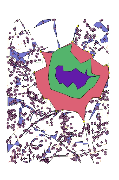
Next, we'll create the actual isochron polygons for each time bin. We must select each set of travel time points using a filter expression for the three time periods: 15 minutes or less, 30 minutes or less, and 45 minutes or less. Then, we'll run the Concave hull tool on each selection. This will create a polygon feature around each set of points.

You'll perform the following steps three times for each of the three break values, which are 15, 30, and 45:

Select isochron_centroids from the Layers panel.
Navigate to Layer | Query.
Click on Clear if there is already a filter expression displayed in the filter expression field of the query dialog.
Provide a specific field expression: cost < [break value] (for example, cost < 15).
Click on OK to select the objects in the layer that matches the expression.
Navigate to Processing Toolbox | Concave hull.
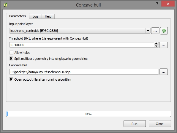
Input the following parameters for Concave hull. All other parameters can be left at their defaults:
- Input point layer: isochron_centroids
- Select Split multipart geometry into singleparts geometries
- Concave hull (the output file) could be similar to c4/data/output/isochron45.shp
- Click on Run, as shown in the following screenshot:

All concave hulls when displayed will look similar to the following image. The "spikiness" of the concave hulls reflects relatively few road segments (points) used to calculate these travel time polygons:

Selecting the travel time ranges in points and creating convex hulls

Previous Chapter

Database importing and topological relationships

Next Chapter

Generating the shortest paths for all students

Table of Contents for QGIS: Becoming a GIS Power User

Creating the travel time isochron polygons

Generating the travel time for each road segment

Creating isochron polygons

Converting the travel time lines to points

Selecting the travel time ranges in points and creating convex hulls

Table of Contents for
QGIS: Becoming a GIS Power User