Table of Contents for
QGIS: Becoming a GIS Power User
 QGIS: Becoming a GIS Power User
Published by
Packt Publishing, 2017
QGIS: Becoming a GIS Power User
Published by
Packt Publishing, 2017
- Cover
- Table of Contents
- QGIS: Becoming a GIS Power User
- QGIS: Becoming a GIS Power User
- QGIS: Becoming a GIS Power User
- Credits
- Preface
- What you need for this learning path
- Who this learning path is for
- Reader feedback
- Customer support
- 1. Module 1
- 1. Getting Started with QGIS
- Running QGIS for the first time
- Introducing the QGIS user interface
- Finding help and reporting issues
- Summary
- 2. Viewing Spatial Data
- Dealing with coordinate reference systems
- Loading raster files
- Loading data from databases
- Loading data from OGC web services
- Styling raster layers
- Styling vector layers
- Loading background maps
- Dealing with project files
- Summary
- 3. Data Creation and Editing
- Working with feature selection tools
- Editing vector geometries
- Using measuring tools
- Editing attributes
- Reprojecting and converting vector and raster data
- Joining tabular data
- Using temporary scratch layers
- Checking for topological errors and fixing them
- Adding data to spatial databases
- Summary
- 4. Spatial Analysis
- Combining raster and vector data
- Vector and raster analysis with Processing
- Leveraging the power of spatial databases
- Summary
- 5. Creating Great Maps
- Labeling
- Designing print maps
- Presenting your maps online
- Summary
- 6. Extending QGIS with Python
- Getting to know the Python Console
- Creating custom geoprocessing scripts using Python
- Developing your first plugin
- Summary
- 2. Module 2
- 1. Exploring Places – from Concept to Interface
- Acquiring data for geospatial applications
- Visualizing GIS data
- The basemap
- Summary
- 2. Identifying the Best Places
- Raster analysis
- Publishing the results as a web application
- Summary
- 3. Discovering Physical Relationships
- Spatial join for a performant operational layer interaction
- The CartoDB platform
- Leaflet and an external API: CartoDB SQL
- Summary
- 4. Finding the Best Way to Get There
- OpenStreetMap data for topology
- Database importing and topological relationships
- Creating the travel time isochron polygons
- Generating the shortest paths for all students
- Web applications – creating safe corridors
- Summary
- 5. Demonstrating Change
- TopoJSON
- The D3 data visualization library
- Summary
- 6. Estimating Unknown Values
- Interpolated model values
- A dynamic web application – OpenLayers AJAX with Python and SpatiaLite
- Summary
- 7. Mapping for Enterprises and Communities
- The cartographic rendering of geospatial data – MBTiles and UTFGrid
- Interacting with Mapbox services
- Putting it all together
- Going further – local MBTiles hosting with TileStream
- Summary
- 3. Module 3
- 1. Data Input and Output
- Finding geospatial data on your computer
- Describing data sources
- Importing data from text files
- Importing KML/KMZ files
- Importing DXF/DWG files
- Opening a NetCDF file
- Saving a vector layer
- Saving a raster layer
- Reprojecting a layer
- Batch format conversion
- Batch reprojection
- Loading vector layers into SpatiaLite
- Loading vector layers into PostGIS
- 2. Data Management
- Joining layer data
- Cleaning up the attribute table
- Configuring relations
- Joining tables in databases
- Creating views in SpatiaLite
- Creating views in PostGIS
- Creating spatial indexes
- Georeferencing rasters
- Georeferencing vector layers
- Creating raster overviews (pyramids)
- Building virtual rasters (catalogs)
- 3. Common Data Preprocessing Steps
- Converting points to lines to polygons and back – QGIS
- Converting points to lines to polygons and back – SpatiaLite
- Converting points to lines to polygons and back – PostGIS
- Cropping rasters
- Clipping vectors
- Extracting vectors
- Converting rasters to vectors
- Converting vectors to rasters
- Building DateTime strings
- Geotagging photos
- 4. Data Exploration
- Listing unique values in a column
- Exploring numeric value distribution in a column
- Exploring spatiotemporal vector data using Time Manager
- Creating animations using Time Manager
- Designing time-dependent styles
- Loading BaseMaps with the QuickMapServices plugin
- Loading BaseMaps with the OpenLayers plugin
- Viewing geotagged photos
- 5. Classic Vector Analysis
- Selecting optimum sites
- Dasymetric mapping
- Calculating regional statistics
- Estimating density heatmaps
- Estimating values based on samples
- 6. Network Analysis
- Creating a simple routing network
- Calculating the shortest paths using the Road graph plugin
- Routing with one-way streets in the Road graph plugin
- Calculating the shortest paths with the QGIS network analysis library
- Routing point sequences
- Automating multiple route computation using batch processing
- Matching points to the nearest line
- Creating a routing network for pgRouting
- Visualizing the pgRouting results in QGIS
- Using the pgRoutingLayer plugin for convenience
- Getting network data from the OSM
- 7. Raster Analysis I
- Using the raster calculator
- Preparing elevation data
- Calculating a slope
- Calculating a hillshade layer
- Analyzing hydrology
- Calculating a topographic index
- Automating analysis tasks using the graphical modeler
- 8. Raster Analysis II
- Calculating NDVI
- Handling null values
- Setting extents with masks
- Sampling a raster layer
- Visualizing multispectral layers
- Modifying and reclassifying values in raster layers
- Performing supervised classification of raster layers
- 9. QGIS and the Web
- Using web services
- Using WFS and WFS-T
- Searching CSW
- Using WMS and WMS Tiles
- Using WCS
- Using GDAL
- Serving web maps with the QGIS server
- Scale-dependent rendering
- Hooking up web clients
- Managing GeoServer from QGIS
- 10. Cartography Tips
- Using Rule Based Rendering
- Handling transparencies
- Understanding the feature and layer blending modes
- Saving and loading styles
- Configuring data-defined labels
- Creating custom SVG graphics
- Making pretty graticules in any projection
- Making useful graticules in printed maps
- Creating a map series using Atlas
- 11. Extending QGIS
- Defining custom projections
- Working near the dateline
- Working offline
- Using the QspatiaLite plugin
- Adding plugins with Python dependencies
- Using the Python console
- Writing Processing algorithms
- Writing QGIS plugins
- Using external tools
- 12. Up and Coming
- Preparing LiDAR data
- Opening File Geodatabases with the OpenFileGDB driver
- Using Geopackages
- The PostGIS Topology Editor plugin
- The Topology Checker plugin
- GRASS Topology tools
- Hunting for bugs
- Reporting bugs
- Bibliography
- Index
We can activate labeling by going to Layer Properties | Labels, selecting Show labels for this layer, and selecting the attribute field that we want to Label with. This is all we need to do to display labels with default settings. While default labels are great for a quick preview, we will usually want to customize labels if we create visualizations for reports or standalone maps.
Using Expressions (the button that is right beside the attribute drop-down list), we can format the label text to suit our needs. For example, the NAME field in our sample airports.shp file contains text in uppercase. To display the airport names in mixed case instead, we can set the title(NAME) expression, which will reformat the name text in title case. We can also use multiple fields to create a label, for example, combining the name and elevation in brackets using the concatenation operator (||), as follows:
title(NAME) || ' (' || "ELEV" || ')'Note the use of simple quotation marks around text, such as ' (', and double quotation marks around field names, such as "ELEV". The dialog will look like what is shown in this screenshot:
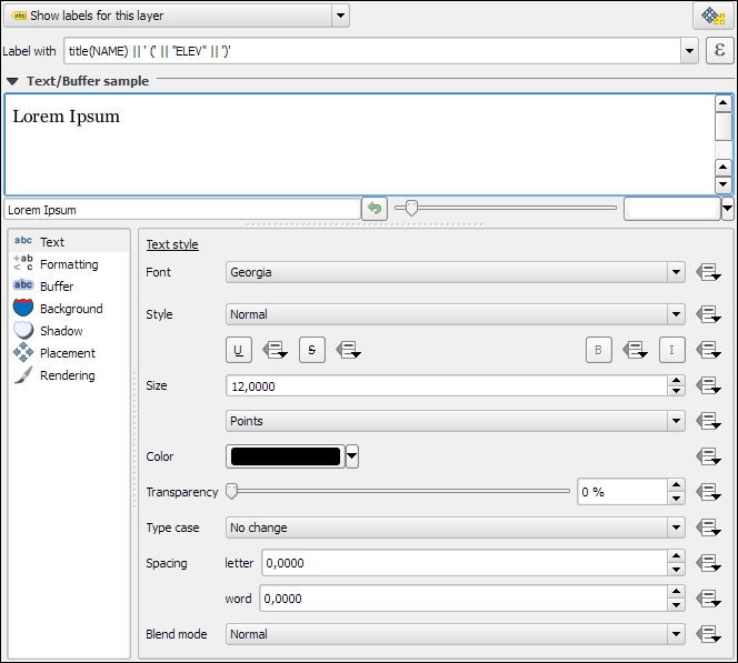
The big preview area at the top of the dialog, titled Text/Buffer sample, shows a preview of the current settings. The background color can be adjusted to test readability on different backgrounds. Under the preview area, we find the different label settings, which will be described in detail in the following sections.
In the Text section (shown in the previous screenshot), we can configure the text style. Besides changing Font, Style, Size, Color, and Transparency, we can also modify the Spacing between letters and words, as well as Blend mode, which works like the layer blending mode that we covered in Chapter 2, Viewing Spatial Data.
Note the column of buttons on the right-hand side of every setting. Clicking on these buttons allows us to create data-defined overrides, similar to those that we discussed at the beginning of the chapter when we talked about advanced vector styling. These data-defined overrides can be used, for example, to define different label colors or change the label size depending on an individual feature's attribute value or an expression.
In the Formatting section, which is shown in the following screenshot, we can enable multiline labels by specifying a Wrap on character. Additionally, we can control Line height and Alignment. Besides the typical alignment options, the QGIS labeling engine also provides a Follow label placement option, which ensures that multiline labels are aligned towards the same side as the symbol the label belongs to:
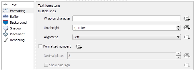
Finally, the Formatted numbers option offers a shortcut to format numerical values to a certain number of Decimal places.
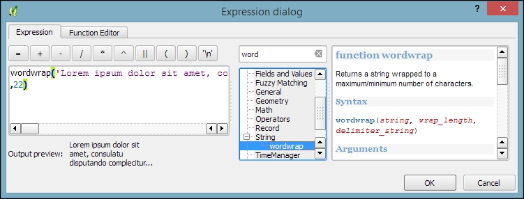
An alternative to wrapping text on a certain character is the wordwrap function, available in expressions. It wraps the input string to a certain maximum or minimum number of characters. The following screenshot shows an example of wrapping a longer piece of text to a maximum of 22 characters per line:
In the Buffer section, we can adjust the buffer Size, Color, and Transparency, as well as Pen join style and Blend mode. With transparency and blending, we can improve label readability without blocking out the underlying map too much, as shown in the following screenshot.
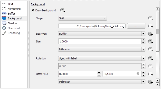
In the Background section, we can add a background shape in the form of a rectangle, square, circle, ellipsoid, or SVG. SVG backgrounds are great for creating effects such as highway shields, which we will discuss shortly.
Similarly, in the Shadow section, we can add a shadow to our labels. We can control everything from shadow direction to Color, Blur radius, Scale, and Transparency.
In the Placement section, we can configure which rules should be used to determine where the labels are placed. The available automatic label placement options depend on the layer geometry type.
For point layers, we can choose from the following:
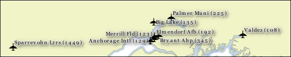
- The flexible Around point option tries to find the best position for labels by distributing them around the points without overlaps. As you can see in the following screenshot, some labels are put in the top-right corner of their point symbol while others appear at different positions on the left (for example, Anchorage Intl (129)) or right (for example, Big Lake (135)) side.
- The Offset from point option forces all labels to a certain position; for example, all labels can be placed above their point symbol.
The following screenshot shows airport labels with a 50 percent transparent Buffer and Drop Shadow, placed using Around point. The Label distance is 1 mm.
For line layers, we can choose from the following placement options:
- Parallel for straight labels that are rotated according to the line orientation
- Curved for labels that follow the shape of the line
- Horizontal for labels that keep a horizontal orientation, regardless of the line orientation
For further fine-tuning, we can define whether the label should be placed Above line, On line, or Below line, and how far above or below it should be placed using Label distance.
For polygon layers, the placement options are as follows:
- Offset from centroid uses the polygon centroid as an anchor and works like Offset from point for point layers
- Around centroid works in a manner similar to Around point
- Horizontal places a horizontal label somewhere inside the polygon, independent of the centroid
- Free fits a freely rotated label inside the polygon
- Using perimeter places the label on the polygon's outline
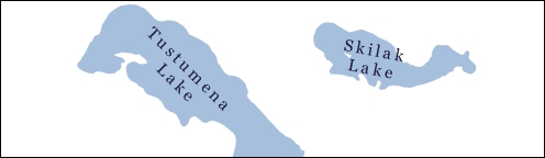
The following screenshot shows lake labels (lakes.shp) using the Multiple lines feature wrapping on the empty space character, Center Alignment, a Letter spacing of 2, and positioning using the Free option:
Besides automatic label placement, we also have the option to use data-defined placement to position labels exactly where we want them to be. In the labeling toolbar, we find tools for moving and rotating labels by hand. They are active and available only for layers that have set up data-defined placement for at least X and Y coordinates:
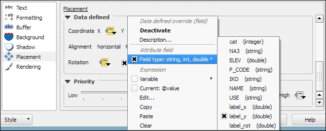
- To start using the tools, we can simply add three new columns,
label_x,label_y, andlabel_rotto, for example, theairports.shpfile. We don't have to enter any values in the attribute table right now. The labeling engine will check for values, and if it finds the attribute fields empty, it will simply place the labels automatically. - Then, we can specify these columns in the label Placement section. Configure the data-defined overrides by clicking on the buttons beside Coordinate X, Coordinate Y, and Rotation, as shown in the following screenshot:
- By specifying data-defined placement, the labeling toolbar's tools are now available (note that the editing mode has to be turned on), and we can use the Move label and Rotate label tools to manipulate the labels on the map. The changes are written back to the attribute table.
- Try moving some labels, especially where they are placed closely together, and watch how the automatically placed labels adapt to your changes.
In the Rendering section, we can define Scale-based visibility limits to display labels only at certain scales and Pixel size-based visibility to hide labels for small features. Here, we can also tell the labeling engine to Show all labels for this layer (including colliding labels), which are normally hidden by default.
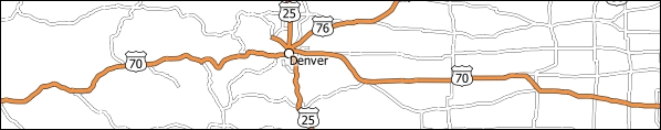
The following example shows labels with road shields. You can download a blank road shield SVG from http://upload.wikimedia.org/wikipedia/commons/c/c3/Blank_shield.svg. Note how only Interstates are labeled. This can be achieved using the Data defined Show label setting in the Rendering section with the following expression:
"level" = 'Interstate'
The labels are positioned using the Horizontal option (in the Placement section). Additionally, Merge connected lines to avoid duplicate labels and Suppress labeling of features smaller than are activated; for example, 5 mm helps avoid clutter by not labeling pieces of road that are shorter than 5 mm in the current scale.
To set up the road shield, go to the Background section and select the blank shield SVG from the folder you downloaded it in. To make sure that the label fits nicely inside the shield, we additionally specify the Size type field as a buffer with a Size of 1 mm. This makes the shield a little bigger than the label it contains.
If you click on Apply now, you will notice that the labels are not centered perfectly inside the shields. To fix this, we apply a small Offset in the Y direction to the shield position, as shown in the following screenshot. Additionally, it is recommended that you deactivate any label buffers as they tend to block out parts of the shield, and we don't need them anyway.