A dynamic web application – OpenLayers AJAX with Python and SpatiaLite

In this section, we will produce our web application, which, unlike any so far, involves a dynamic interaction between client and server. We will also use a different web map client API—OpenLayers. OpenLayers has long been a leader in web mapping; however, it has been overshadowed by smaller clients, such as Leaflet, as of late. With its latest incarnation, OpenLayers 3, OpenLayers has been slimmed down but still retains a functionality advantage in most areas over its newer peers.

Server side – CGI in Python

Common Gateway Interface (CGI) is perhaps the simplest way to run a server-side code for dynamic web use. This makes it great for doing proof of concept learning. The most typical use of CGI is in data processing and passing it onto the database from the web forms received through HTTP POST. The most common attack vector is the SQL injection. Going a step further, dynamic processing similar to CGI is often implemented through a minimal framework, such as Bottle, CherryPy, or Flask, to handle common tasks such as routing and sometimes templating, thus making for a more secure environment.

Don't forget that Python is sensitive to indents. Indents are always expressed as spaces with a uniform number per hierarchy level. For example, an if block may contain lines prefixed by four spaces. If the if block falls within a for loop, the same lines should be prefaced by 8 spaces.

Python CGI development

Next, we will start up a CGIHTTPServer hosting instance via a separate Windows console session. Then, we will work on the development of our server-side code—primarily through the QGIS Python Console.

Starting a CGI hosting

Starting a CGI session is simple— you just need to use the –m command line switch directly with Python, which loads the module as you might load a script. The following code starts CGIHTTPServer in port 8000. The current working directory will be served as the public web directory; in this case, this is C:\packt\c6\data\web.

In a new Windows console session, run the following:

cd C:\packt\c6\data\web
python -m CGIHTTPServer 8000

Testing the CGI hosting

Python (.py) CGI files can only run out of directories named either cgi or cgi-bin. This is a precaution to ensure that we intend the files in this directory to be publically executable.

To test this, create a file at c6/data/web/cgi-bin/simple_test.py with the following content:

Note

The first line is our shebang, which allows this file to be independently executable through the interpreter listed in the path on Unix systems. While this has no effect on Windows systems, where execution is handled through file associations, we will leave this here for interoperability.

#!/usr/bin/python

# Import the cgi, and system modules
import cgi, sys

# Required header that tells the browser how to render the HTML.
print "Content-Type: text/html\n\n"
print "Hello world"

You should now see the "Hello world" message when you visit http://localhost:8000/cgi-bin/simple_test.py on your browser. To debug on the client side, make sure you are using a browser-based web development view, plugin, or extension, such as Chrome's Developer Tools toolbar or Firefox's Firebug extension.

Debugging server-side code

Here are a few ways through which you can debug during Python CGI development:

Use the Python Console in QGIS (navigate to Plugins | Python Console). You can run the Python code from your Python CGI Scripts here directly; however, this will fail for the scripts that rely on information passed through HTTP, but you can at least catch syntax errors, and you can populate it with the expected values to compare the result to what you're getting on a web browser. Sometimes, you'll want to quit QGIS to clear out the memory of the Python interpreter.
A quicker way of doing this is to run your script in the command line with –d (verbose debugging). This will catch any issues that may not come up in interactive use, avoiding the variables that may have inadvertently been set in the same interactive session (substitute index.py with the name of your Python script). Run the following command from your command line shell:
```
python -d C:\packt\c6\data\web\cgi-bin\index.py
```
If your Python CGI script is interacting with a database, you definitely need to test the queries through DB Manager SQL Window (or whichever database interface you prefer). It is often helpful to populate the queries with the expected values.
Go to the following location in our web browser (substitute index.py with the name of your Python script):
localhost:8000/cgi-bin/index.py

Our Python server-side, database-driven code

Now, let's create a Python code to provide dynamic web access to our SQLite database.

PySpatiaLite

The PySpatiaLite module provides dbapi2 access to SpatiaLite databases. Dbapi2 is a standard library for interacting with databases from Python. This is very fortunate because if you use the dbapi2 connector from the sqlite3 module alone, any query using spatial types or functions will fail. The sqlite3 module was not built to support SpatiaLite.

Add the following to the preceding code. This will perform the following functions:

Import the PySpatiaLite module and connect to our sqlite3/SpatiaLite database
Use the connection as a context manager, which automatically commits the executed queries and rolls back in case of an error
To test that the connection is working, use the SQLITE_VERSION() function in a SELECT query and print the result

The following code, appended to the preceding one, can be found at c6/data/web/cgi-bin/db_test.py. Make sure that the path in the code for the SQLite database file matches the actual location on your system.

# Import the pySpatiaLite module
from pySpatiaLite import dbapi2 as sqlite3
conn = sqlite3.connect('C:\packt\c6\data\web\cgi-bin\c6.sqlite')

# Use connection handler as context
with conn:    
  c = conn.cursor() 
  c.execute('SELECT SQLITE_VERSION()')

  data = c.fetchone()
  print data
  print 'SQLite version:{0}'.format(data[0])

You can view the following results in a web browser at http://localhost:8000/cgi-bin/db_test.py.

(u'3.7.17',) SQLite version:3.7.17

The first time that the data is printed, it is preceded by a u and wrapped in single quotes. This tells us that this is a unicode string (as our database uses unicode encoding). If we access element 0 in this string, we get a nonwrapped result.

The Python code for web access to SQLite through JSON

The following code performs the following functions:

It connects to the database
It issues a query to find the minimum distance location and field where the specified location and date are given
It returns JSON with field value pairs based on the database result field names and values

You can find the code at c6/data/web/cgi-bin/get_json.py:

#!/usr/bin/python

import cgi, cgitb, json, sys
from pySpatiaLite import dbapi2 as sqlite3

# Enables some debugging functionality
cgitb.enable()

# Creating row factory function so that we can get field names
# in dict returned from query
def dict_factory(cursor, row):
  d = {}
  for idx, col in enumerate(cursor.description):
    d[col[0]] = row[idx]
  return d

# Connect to DB and setup row_factory
conn = sqlite3.connect('C:\packt\c6\data\web\cgi-bin\c6.sqlite')
conn.row_factory = dict_factory

# Print json headers, so response type is recognized and correctly decoded
print 'Content-Type: application/json\n\n'

# Use CGI FieldStorage object to retrieve data passed by HTTP GET
# Using numeric datatype casts to eliminate special characters
fs = cgi.FieldStorage()
longitude = float(fs.getfirst('longitude'))
latitude = float(fs.getfirst('latitude'))
day = int(fs.getfirst('day'))

# Use user selected location and days to find nearest location (minimum distance) 
# and correct date column
query = 'SELECT pk, calc{2} as index_value, min(Distance(PointFromText(\'POINT ({0} {1})\'),geom)) as min_dist FROM vulnerability'.format(longitude, latitude, day)

# Use connection as context manager, output first/only result row as json
with conn:
  c = conn.cursor()
  c.execute(query)
  data = c.fetchone()
  print json.dumps(data)

You can test the preceding code by commenting out the portion that gets arguments from the HTTP request and setting these arbitrarily.

The full code is available at c6/data/web/cgi-bin/json_test.py:

# longitude = float(fs.getfirst('longitude'))
# latitude = float(fs.getfirst('latitude'))
# day = int(fs.getfirst('day'))
longitude = -75.28075
latitude = 39.47785
day = 15

If you browse to http://localhost:8000/cgi-bin/json_test.py, you'll see the literal JSON printed to the browser. You can also do the equivalent by browsing to the following URL, which includes these arguments: http://localhost:8000/cgi-bin/get_json.py?longitude=-75.28075&latitude= 39.47785&day=15.

{"pk": 260, "min_dist": 161.77454362713507, "index_value": 7}

The OpenLayers/jQuery client-side code

Now that our backend code and dependencies are all in place, it's time to move on to integrating this into our frontend interface.

Exporting the OpenLayers 3 map using QGIS

QGIS helps us get started on our project by allowing us to generate a working OpenLayers map with all the dependencies, basic HTML elements, and interaction event handler functionality. Of course, as with qgis2leaf, this can be extended to include the additional leveraging of the map project layers and interactivity elements.

The following steps will produce an OpenLayers 3 map that we will modify to produce our database-interactive map application:

Start a new QGIS map or remove all the layers from the current one.
Add delaware_boundary.shp to the map. Pan and zoom to the Delaware geographic boundary object if QGIS does not do so automatically.
Convert the delaware_boundary polygon layer to lines by navigating to Vector | Geometry Tools | Polygons to lines. Nonfilled polygons are not supported by Export to OpenLayers. The following image shows these inputs populated: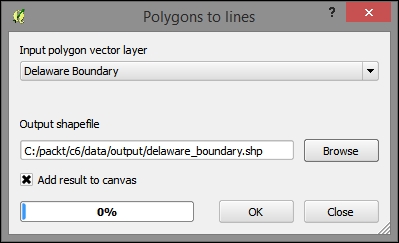
After you add the line boundaries, brighten them up and increase the size as well. Clicking on anything outside this boundary may not return a valid result. Rename the layer Delaware Boundary in the Layers panel.
Install the Export to OpenLayers 3 plugin if it isn't already installed.
Navigate to Web | Export to OpenLayers | Create OpenLayers Map.
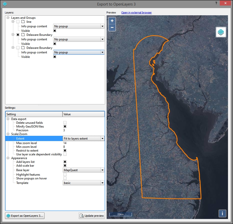
In the Export to OpenLayers 3 dialog, use the following parameter values (refer to the following image for clarification):
- Ensure that your stylized line boundary for Delaware (which we created in step 4) is checked and visible with no popup. Otherwise, this might obscure the interaction that we will create.
- Delete the unused fields. This is an important step, so uncheck this. Otherwise, you may see an error.
- If you've already zoomed and panned your canvas to the Delaware Boundary layer, you can ignore the Extent parameter. Otherwise, set the extent parameter to Fit to Layers extent.
- Max zoom level: 14.
- Min zoom level: 8.
- Select Restrict to extent.
- Unselect Use layer scale dependent visibility.
- Base layer: MapQuest, as shown in the following screenshot:

Modifying the exported OpenLayers 3 map application

Now that we have the base code and dependencies for our map application, we can move on to modifying the code so that it interacts with the backend, providing the desired information upon click interaction.

Remember that the backend script will respond to the selected date and location by finding the closest "regular point" and the calculated interpolated index for that date.

Adding an interactive HTML element

Add the following to c6/data/web/index.html in the body, just above the div#id element.

This is the HTML for the select element, which will pass a day. You would probably want to change the code here to scale with your application—this one is limited to days in a single month (and as it requires 10 days of retrospective data, it is limited to days from 6/10 to 6/30):

  <select id="day">
    <option value="10">2013-06-10</option>
    <option value="11">2013-06-11</option>
    <option value="12">2013-06-12</option>
    <option value="13">2013-06-13</option>
    <option value="14">2013-06-14</option>
    <option value="15">2013-06-15</option>
    <option value="16">2013-06-16</option>
    <option value="17">2013-06-17</option>
    <option value="18">2013-06-18</option>
    <option value="19">2013-06-19</option>
    <option value="20">2013-06-20</option>
    <option value="21">2013-06-21</option>
    <option value="22">2013-06-22</option>
    <option value="23">2013-06-23</option>
    <option value="24">2013-06-24</option>
    <option value="25">2013-06-25</option>
    <option value="26">2013-06-26</option>
    <option value="27">2013-06-27</option>
    <option value="28">2013-06-28</option>
    <option value="29">2013-06-29</option>
    <option value="30">2013-06-30</option>
  </select>

This element will then be accessed by jQuery using the div#id reference.

AJAX – the glue between frontend and backend

AJAX is a loose term applied specifically to an asynchronous interaction between client and server software using XML objects. This makes it possible to retrieve data from the server without the classic interaction of a submit button, which will take you to a page built on the result. Nowadays, AJAX is often used with JSON instead of XML to the same affect; it does not require a new page to be generated to catch the result from the server-side processing.

jQuery is a JavaScript library which provides many useful cross-browser utilities, particularly focusing on the DOM manipulation. One of the useful features that jQuery is known for is sending, receiving, and rendering results from AJAX calls. AJAX calls used to be possible from within OpenLayers; however, in OpenLayers 3, an external library is required. Fortunately for us, jQuery is included in the exported base OpenLayers 3 web application from QGIS.

Adding an AJAX call to the singleclick event handler

To add a jQuery AJAX call to our CGI script, add the following code to the "singleclick" event handler on SingleClick. This is our custom function that is triggered when a user clicks on the frontend map.

This AJAX call references the CGI script URL. The data object contains all the parameters that we wish to pass to the server. jQuery will take care of encoding the data object in a URL query string. Execute the following code:

jQuery.ajax({ 
  url: http://localhost:8000/cgi-bin/get_json.py,
  data: {"longitude": newCoord[0], "latitude": newCoord[1], "day": day}
})
Add a callback function to the jquery ajax call by inserting the following lines directly after it.
.done(function(response) {
popupText = 'Vulnerability Index (1=Least Vulnerable, 10=Most Vulnerable): ' + response.index_value;

Populating and triggering the popup from the callback function

Now, to get the script response to show in a popup after clicking, comment out the following lines:

/* var popupField;

  var currentFeature;
  var currentFeatureKeys;
  map.forEachFeatureAtPixel(pixel, function(feature, layer) {
    currentFeature = feature;
    currentFeatureKeys = currentFeature.getKeys();
    var field = popupLayers[layersList.indexOf(layer) - 1];
    if (field == NO_POPUP){
    }
    else if (field == ALL_FIELDS){
      for ( var i=0; i<currentFeatureKeys.length;i++) {
        if (currentFeatureKeys[i] != 'geometry') {
          popupField = currentFeatureKeys[i] + ': '+ currentFeature.get(currentFeatureKeys[i]);
          popupText = popupText + popupField+'<br>';
        }
      }
    }
    else{
      var value = feature.get(field);
      if (value){
        popupText = field + ': '+ value;
      }
    }
  }); */

Finally, copy and paste the portion that does the actual triggering of the popup in the .done callback function. The .done callback is triggered when the AJAX call returns a data response from the server (the data response is stored in the response object variable). Execute the following code:

.done(function(response) {
  popupText = 'Vulnerability Index (1=Least Vulnerable, 10=Most Vulnerable): ' + response.index_value;  
  if (popupText) {
    overlayPopup.setPosition(coord);
    content.innerHTML = popupText;
    container.style.display = 'block';
  } else {
    container.style.display = 'none';
   closer.blur();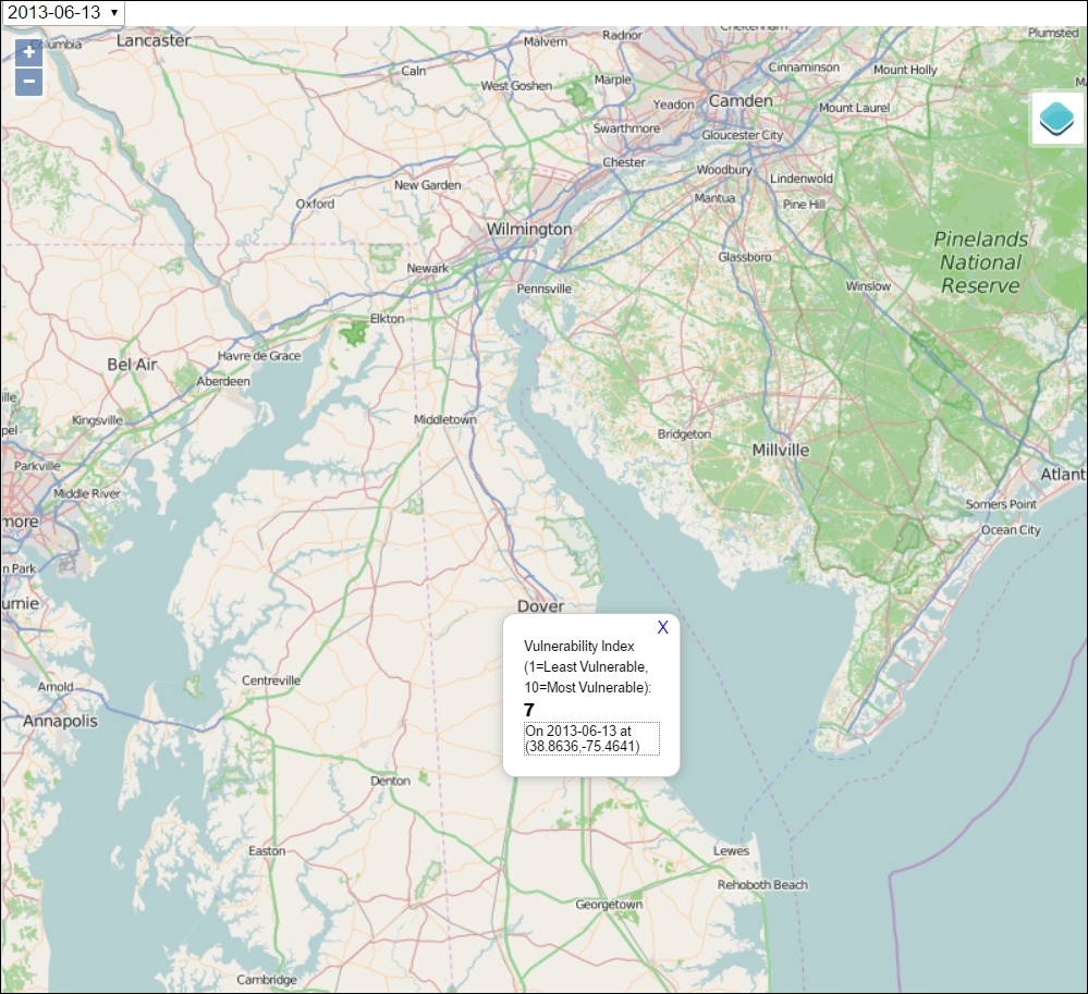
  }

Testing the application

Now, the application should be complete. You will be able to view it in your browser at http://localhost:8000.

You will want to test by picking a date from the Select menu and clicking on different locations on the map. You will see something similar to the following image, showing a susceptibility score for any location on the map within the study extent (Delaware).