Chapter 3. Discovering Physical Relationships

In this chapter, we will create an application for a raster physical modeling example. First, we'll use a raster analysis to model the physical conditions for some basic hydrological analysis. Next, we'll redo these steps using a model automation tool. Then, we will attach the raster values to the vector objects for an efficient lookup in a web application. Finally, we will use a cloud platform to enable a dynamic query from the client-side application code. We will take a look at an environmental planning case, providing capabilities for stakeholders to discover the upstream toxic sites.

In this chapter, we will cover the following topics:

Hydrological modeling
Workflow automation with graphical models
Spatial relationships for a performant access to information
The NNJoin plugin
The CartoDB cloud platform
Leaflet SQLQueries using an external API:CartoDB

Hydrological modeling

The behavior of water is closely tied with the characteristics of the terrain's surface—particularly the values connected to elevation. In this section, we will use a basic hydrological model to analyze the location and direction of the hydrological network—streams, creeks, and rivers. To do this, we will use a digital elevation model and a raster grid, in which the value of each cell is equal to the elevation at that location. A more complex model would employ additional physical parameters (e.g., infrastructure, vegetation, etc.). These modeling steps will lay the necessary foundation for our web application, which will display the upstream toxic sites (brownfields), both active and historical, for a given location.

There are a number of different plugins and Processing Framework algorithms (operations) that enable hydrological modeling. For this exercise, we will use SAGA algorithms, of which many are available, with some help from GDAL for the raster preparation. Note that you may need to wait much longer than you are accustomed to for some of the hydrological modeling operations to finish (approximately an hour).

Preparing the data

Some work is needed to prepare the DEM data for hydrological modeling. The DEM path is c3/data/original/dem/dem.tif. Add this layer to the map (navigate to Layer | Add Layer | Add Raster Layer). Also, add the county shapefile at c3/data/original/county.shp (navigate to Layer | Add Layer | Add Vector Layer).

Filling the grid sinks

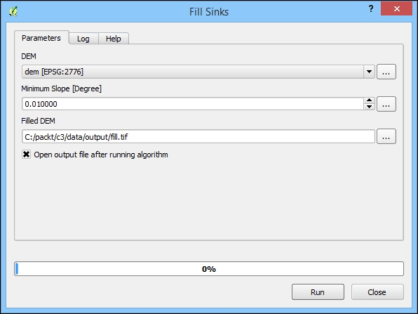
Filling the grid sinks smooths out the elevation surface to exclude the unusual low points in the surface that would cause the modeled streams to—unrealistically—drain to these local lows instead of to larger outlets. The steps to fill the grid sinks are as follows:

Navigate to Processing Toolbox (Advanced Interface).
Search for Fill Sinks (under SAGA | Terrain Analysis | Hydrology).
Run the Fill Sinks tool.
In addition to the default parameters, define DEM as dem and Filled DEM as c3/data/output/fill.tif.
Click on Run, as shown in the following screenshot:

Clipping the grid to study the area by mask layer

By limiting the raster processing extent, we exclude the unnecessary data, improving the speed of the operation. At the same time, we also output a more useful grid that conforms to our extent of interest. In QGIS/SAGA, in order to limit the processing to a fixed extent or area, it is necessary to eliminate those cells from the grid—in other words, the setting cells outside the area or extent, which are sometimes referred to as NoData (or no-data, and so on) in raster software, to a null value.

Tip

Unlike ArcGIS or GRASS, the SAGA package under QGIS does not have any capability to set an extent or area within which we want to limit the raster processing.

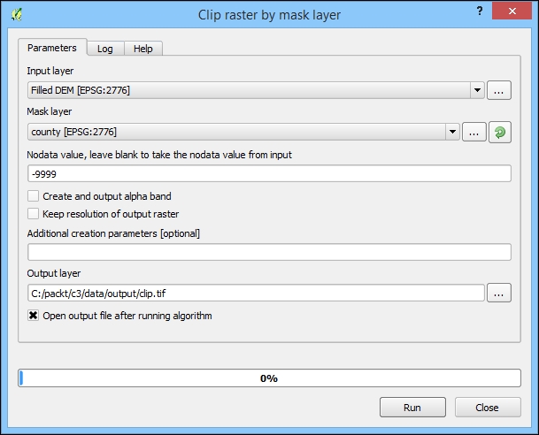
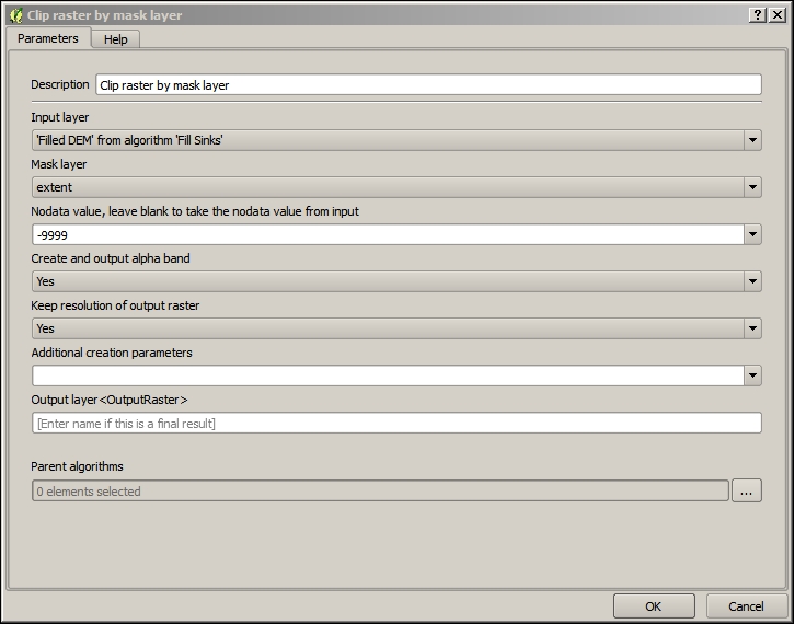
In QGIS, the raster processing's extent limitation can be accomplished using a vector polygon or a set of polygons with the Clip raster by mask layer tool. By following the given steps, we can achieve this:

Navigate to Processing Toolbox (Advanced Interface).
Search for Mask (under GDAL | Extraction).
Run the Clip raster by mask layer tool.
Enter the following parameters, keeping others as default:
- Input layer: This is the layer corresponding to fill.tif, created in the previous Fill Sinks section
- Mask layer: county
- Output layer: c3/data/output/clip.tif
Click on Run, as shown in the following screenshot:

Note

This function is not available in some versions of QGIS for Mac OS.

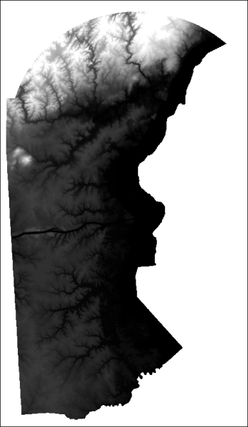
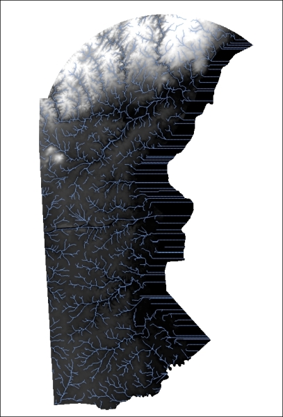
The output from Clip by mask layer tool, showing the grid clipped to the county polygon, will look similar to the following image (the black and white color gradient or mapping to a null value may be reversed):

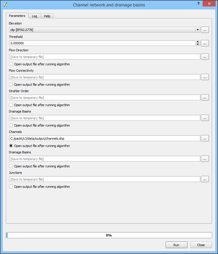
Clipping the grid to study the area by mask layer

Modeling the hydrological network based on elevation

Now that our elevation grid has been prepared, it is time to actually model the hydrological network location and direction. To do this, we will use Channel network and drainage basins, which only requires a single input: the (filled and clipped) elevation model. This tool will produce the hydrological lines using a Strahler Order threshold, which relates to the hierarchy level of the returned streams (for example, to exclude very small ditches) The default of 5 is perfect for our purposes, including enough hydrological lines but not too many. The results look pretty realistic. This tool also produces many additional related grids, which we do not need for this project. Perform the following steps:

Navigate to Processing Toolbox (Advanced Interface).
Search for Channel network and drainage basins (under SAGA | Terrain Analysis | Hydrology).
Run the Channel network and drainage basins tool.
In the Elevation field, input the filled and clipped DEM, given as the output in the previous section.
In the Threshold field, keep it at the default value (5.0).
In the Channels field, input c3/data/output/channels.shp.
Ensure that Open output file after running algorithm is selected
Unselect Open output file after running algorithm for all other outputs.
Click on Run, as shown in the following screenshot:

The output from the Channel network and drainage basins, showing the hydrological line location, will look similar to the following image:

Modeling the hydrological network based on elevation

Workflow automation with the graphical models

Graphical Modeler is a tool within QGIS that is useful for modeling and automating workflows. It differs from batch processing in that you can tie together many separate operations in a processing sequence. It is considered a part of the processing framework. Graphical Modeler is particularly useful for workflows containing many steps to be repeated.

By building a graphical model, we can operationalize our hydrological modeling process. This provides a few benefits, as follows:

Our modeling process is graphically documented and preserved
The model can be rerun in its entirety with little to no interaction
The model can be redistributed
The model is parameterized so that we could rerun the same process on different data layers

Creating a graphical model

Bring up the Graphical Modeler dialog from the Processing menu.
1. Navigate to Processing | Graphical Modeler.
Enter a model name and a group name.
Save your model under c3/data/output/c3.model.
The dialog is modal and needs to be closed before you can return to other work in QGIS, so saving early will be useful.

Adding the input parameters

Some of the inputs to your model's algorithms will be the outputs of other model algorithms; for others, you will need to add a corresponding input parameter.

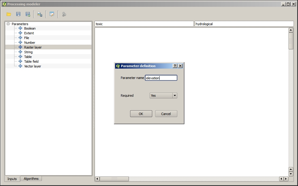
Adding the raster parameter – elevation

We will add the first data input parameter to the model so that it is available to the model algorithms. It is our original DEM elevation data. Perform the following steps:

Select the Inputs tab from the lower left corner of the Processing modeler display.
Drag Raster layer from the parameters list into the modeler pane. This parameter will represent our elevation grid (DEM).
Input elevation for Parameter name.
Click on OK, as shown in the following screenshot:

Adding the vector parameter – extent

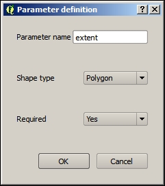
We will add the next data input parameter to the model so that it is available to the model algorithms. It is our vector county data and the extent of our study.

Add a vector layer for our extent polygon (county). Make sure you select Polygon as the type, and call this parameter extent.
You will need to input a parameter name. It would be easiest to use the same layer/parameter names that we have been using so far, as shown in the following screenshot:

Adding the algorithms

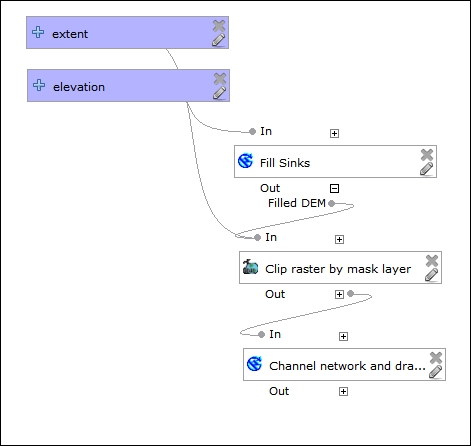
The modeler connects the individual with their input data and their output data with the other algorithms. We will now add the algorithms.

Fill Sinks

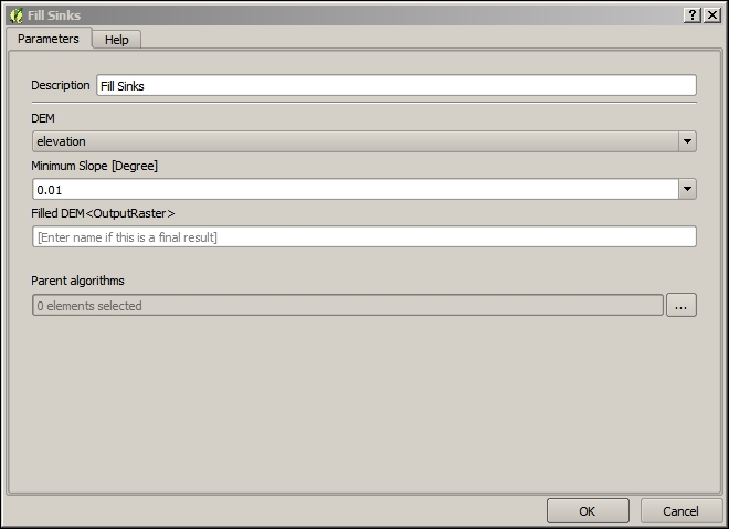
The first algorithm we will add is Fill Sinks, which as we noted earlier, removes the problematic low elevations from the elevation data. Perform the following steps:

Select the Algorithms tab from the lower-left corner.
After you drag in an algorithm, you will be prompted to choose the parameters.
Use the search input to locate Fill Sinks and then open.
Select elevation for the DEM parameter and click on OK, as shown in the following screenshot:

Clip raster

The next algorithm we will add is Clip raster by mask layer, which we've used to limit the processing extent of the subsequent raster processing. Perform the following steps:

Use the search input to locate Clip raster by mask layer.
Select 'Filled DEM' from algorithm 'Fill Sinks' for the Input layer parameter.
Select extent for the Mask layer parameter.
Click on OK, accepting the other parameter defaults, as shown in the following screenshot:

Channel network and drainage basins

The final algorithm we will add is Channel network and drainage basins, which produces a model of our hydrological network. Perform the following steps:

Use the search input to locate Channel network and drainage basins.
Select 'Output Layer' from algorithm 'Clip raster by mask layer' for the Elevation parameter.
Click on OK, accepting the other parameter defaults.
Once you populate all the three algorithms, your model will look similar to the following image:

Running the model

Now that our model is complete, we can execute all the steps in an automated sequential fashion:

Run your model by clicking on the Run model button on the right-hand side of the row of buttons.
You'll be prompted to select values for the elevation and the extent input layer parameters you defined earlier. Select the dem and county layers for these inputs, respectively, as shown in the following screenshot: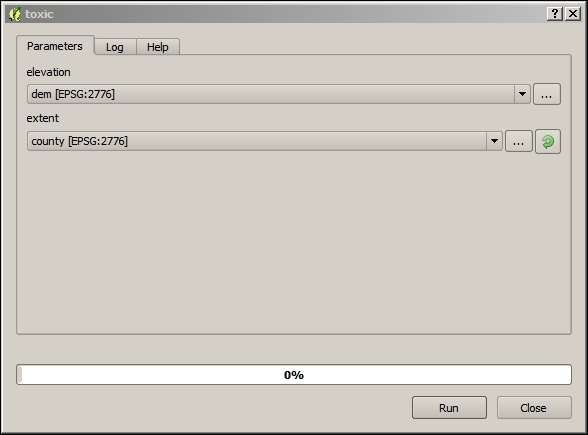
After you define and run your model, all the outputs you defined earlier will be produced. These will be located at the paths that you defined in the parameters dialog or in the model algorithms themselves.