The CartoDB platform

CartoDB is a cloud-based GIS platform which provides data management, query, and visualization capabilities. CartoDB is based on Postgres/PostGIS in the backend, and one of the most exciting functions of this platform is the ability to pass spatial queries using PostGIS syntax via the URL and HTTP API.

Publishing the data to CartoDB

To publish the data to CartoDB, you'll first need to establish an account. You can easily do this with the Google Single sign-in or create your own account with a username and password. CartoDB offers free accounts, which are usable for an unlimited amount time. You are limited to 50 MB of data storage and all the data published will be publically viewable. Once you've signed up, you can upload the layer produced in the previous section. Perform the following steps:

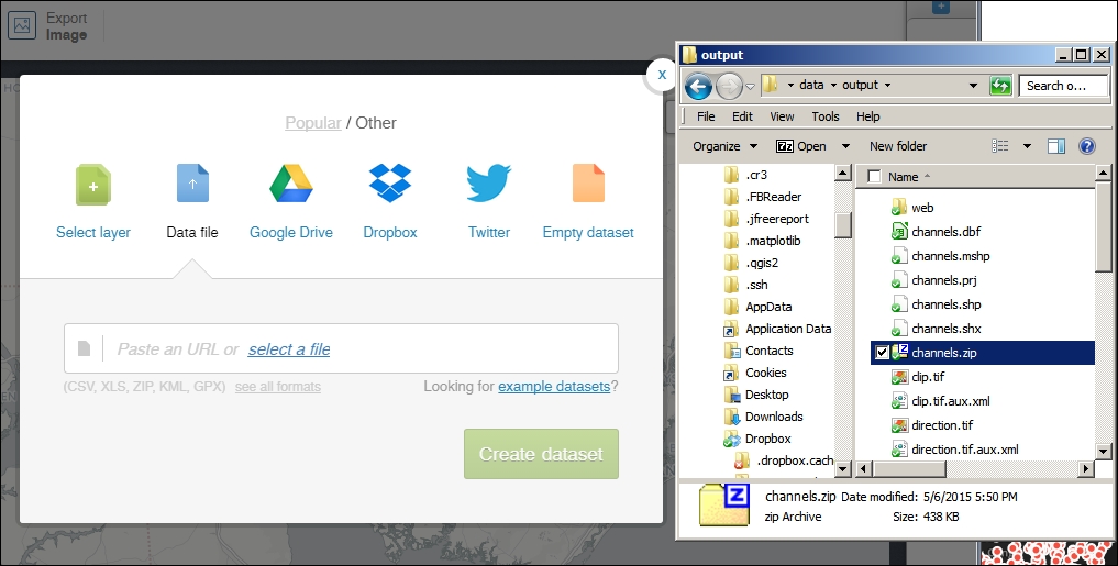
Zip up the shapefile-related files, at c3/data/output/channels.* and c3/data/output/toxic_channels.*, to prepare them for upload to CartoDB.
Log in at https://cartodb.com/login if you haven't already done so.
You should be redirected to your dashboard page after login. Select New Map from this page.
Click on Create New Map to start a new map from scratch.
Click on Connect dataset under Add dataset to add the datasets from your local machine.
Browse c3/data/output/channels.zip and c3/data/output/toxic_channels.zip and add these to the map.
Select the datasets you would like to add to the map.
Select Create Map.

Preparing a CartoDB SQL Query

SQL is the lingua franca of database queries through which you can do anything from filtering to spatial operations to manipulating data on the database. There are slight differences in the way SQL works from one database system to the next one. The CartoDB SQL queries use valid Postgres/PostGIS syntax. For more information on Postgres/PostGIS SQL, check out the reference chapter in the manuals for Postgres (http://www.postgresql.org/docs/9.4/interactive/reference.html) for general functions and PostGIS (http://postgis.net/docs/manual-2.1/reference.html) for spatial functions.

There are a few different ways in which you can test your queries against CartoDB—each involving a different ease of input and producing a different result type.

Generating the test data

Our SQL query only requires one parameter that we do not know ahead of time: the coordinates of the user-selected click location. To simulate this interaction with QGIS and generate a coordinate pair, we will use the Coordinate Capture plugin. Perform the following steps:

Install the Coordinate Capture plugin if you have not already done so.
From the Vector menu, display the Coordinate Capture panel (navigate to Vector | Coordinate Capture | Coordinate Capture).
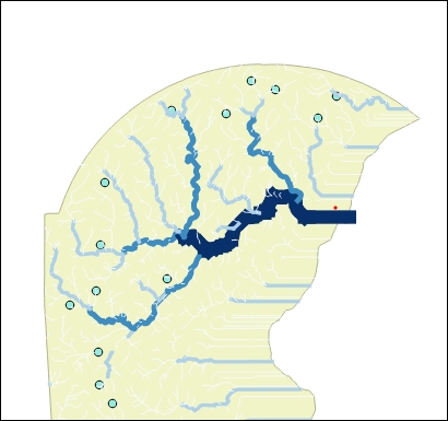
Select Start capture from the Coordinate Capture panel.
Click on a place on the map that you would expect to see upstream results for. In other words, based on the elevation surface, select a low point near a hydrological line; other hydrological objects should run down into that point, as shown in the following image:
Record the coordinates displayed in the Coordinate Capture panel, as shown in the following screenshot:

The CartoDB SQL view tab

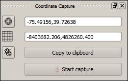
Now, we will return to CartoDB in a web browser to run our first test.

While this method is probably the most straightforward in terms of data entry, it is limited to producing results via the map. There are no text results produced besides errors, which limits your ability to test and debug. Perform the following steps:

On your map, click on the tab corresponding to the toxic_channels layer. This is often accessed on the tab marked 2 on the right-hand side.
You should see the SQL view tab displayed by default with a SQL input area.
The SQL query given in the following section selects all the records from our joined table, which contains the location of toxic sites with their closest hydrological basin and stream order that fulfill the following criteria based on the coordinates we pass:
- It is in the same hydrological basin as the passed coordinates.
- It has a lower hydrological stream order than the closest stream to the passed coordinates.
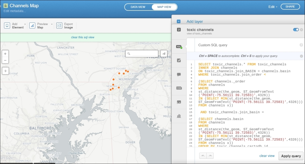
  Recall that we generated test coordinates to pass with the Coordinate Capture plugin in the last step. Enter the following into the SQL area. This query will select all the fields from toxic_channels as expressed with the wildcard symbol (*) using various subqueries, joins, and spatial operations. The end result will show all the toxic sites that are upstream from the clicked point in its basin (code in c3/data/original/query1.sql). Execute the following code:
```
SELECT toxic_channels.* FROM toxic_channels
INNER JOIN channels 
ON toxic_channels.join_BASIN = channels.basin
WHERE toxic_channels.join_order <

(SELECT channels._order 
FROM channels
WHERE 
st_distance(the_geom, ST_GeomFromText
('POINT(-75.56111 39.72583)',4326)) 
IN (SELECT MIN(st_distance(the_geom, 
ST_GeomFromText('POINT(-75.56111 39.72583)',4326)))
FROM channels x))

 AND toxic_channels.join_basin = 

(SELECT channels.basin 
FROM channels
WHERE 
st_distance(the_geom, ST_GeomFromText
('POINT(-75.56111 39.72583)',4326)) 
IN (SELECT MIN(st_distance(the_geom, 
ST_GeomFromText('POINT(-75.56111 39.72583)',4326)))
FROM channels x))
GROUP BY toxic_channels.cartodb_id
```
Select Apply Query to run the query.

If the query runs successfully, you should see an output similar to the following image:

Note

The following errors may confound the efforts to debug and test via the CartoDB SQL tab:

Error at the end of a statement: A semi-colon, while valid, causes an error in this interface.
Does not contain cartodb_id: The statement must explicitly contain a cartodb_id field so that it does not generate this error. However, this error does not typically affect the use through the API or URL parameters.
Does not contain the_geom: The statement must explicitly contain a reference to the the_geom column even though this column is not visible within your cartodb table, to map the result.

Sometimes, the SQL input area is "sticky". If this happens, just "clear view".

The QGIS CartoDB plugin

Next, let's test the SQL from within QGIS using the QGIS CartoDB Plugin. Perform the following steps:

Install the QGIS CartoDB plugin, QGISCartoDB.
Open the SQL CartoDB dialog and navigate to Web | CartoDB Plugin | Add SQL CartoDB Layer.
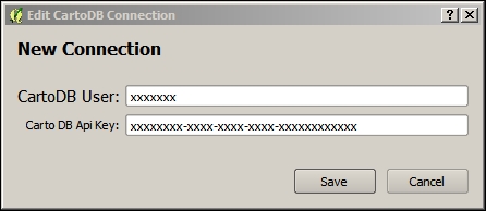
Establish a connection to your CartoDB account:
1. Click on New.
2. Locate and enter your username and API key from your account in a browser. The query you ran earlier will be saved so you can do this in the open tab (if it is still open). Otherwise, navigate back to CartoDB. Your account name can be found in the URL when you are logged into CartoDB, where the username is in username.cartodb.com/*. You can find your API key by clicking on your avatar from your dashboard and selecting Your API keys.
3. Click on Save, as shown in the following screenshot:
Now that you are connected to your CartoDB account, load tables from the CartoDB SQL Layer dialog.
Enter the preceding SQL statement in the SQL Query area. You can use the Tables section of the Add CartoDB SQL Layer dialog to view the field names and datatypes in your query.
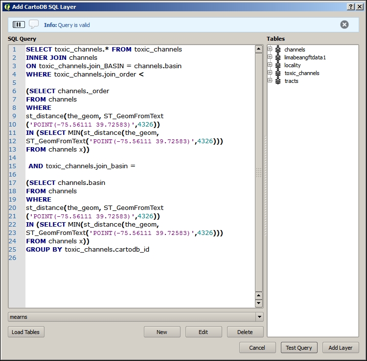
Click on Test Query to test the syntax against CartoDB. Refer to the info box in the previous test section for some common confounding errors you may experience with the CartoDB SQL interface.
Click on Add Layer to add the result to QGIS.

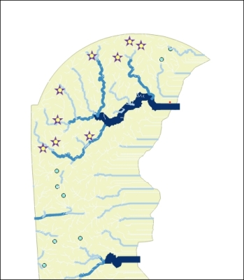
The layer added from these steps will give you the location of the toxic sites upstream from the chosen coordinate. If you symbolized these locations with stars and streams according to their upstream/downstream rank, you would see something similar to the following image:

The CartoDB SQL API

If you want to see the actual contents returned by a CartoDB SQL query in the JSON format, the best way to do so is by sending your SQL statement to the CartoDB SQL API endpoint at http://[YOURUSERNAME].cartodb.com/api/v2/sql. This can be useful to debug issues in interaction with your web application in particular.

The browser string uses an encoded URL, which substitutes character sequences for some special characters. For example, you could use a URL encoder/decoder, which is easily found on the Web, to produce such a string.

Use the following instructions to see the result JSON returned by CartoDB given a particular SQL query. The URL string is also contained in c3/data/original/url_query1.txt.

Enter the following URL string into your browser, substituting [YOURUSERNAME] with your CartoDB user name and [YOURAPIKEY] with your API key:

http://[YOURUSERNAME].cartodb.com/api/v2/sql?q=%20SELECT%20toxic_channels.*%20FROM%20toxic_channels%20INNER%20JOIN%20channels%20ON%20toxic_channels.join_BASIN%20=%20channels.basin%20WHERE%20toxic_channels.join_order%20%3C%20(SELECT%20channels._order%20FROM%20channels%20WHERE%20st_distance(the_geom,%20ST_GeomFromText%20(%27POINT(-75.56111%2039.72583)%27,4326))%20IN%20(SELECT%20MIN(st_distance(the_geom,%20ST_GeomFromText(%27POINT(-75.56111%2039.72583)%27,4326)))%20FROM%20channels%20x))%20AND%20toxic_channels.join_basin%20=%20(SELECT%20channels.basin%20FROM%20channels%20WHERE%20st_distance(the_geom,%20ST_GeomFromText%20(%27POINT(-75.56111%2039.72583)%27,4326))%20IN%20(SELECT%20MIN(st_distance(the_geom,%20ST_GeomFromText(%27POINT(-75.56111%2039.72583)%27,4326)))%20FROM%20channels%20x))%20GROUP%20BY%20toxic_channels.cartodb_id%20&api_key=[YOURAPIKEY]

Submit the browser request.

You will see a result similar to the following:

{"rows":[{"the_geom":"0101000020E610000056099A6A64E352C0B23A9C05D4E84340","id":13,"join_segme":1786,"join_node_":1897,"join_nod_1":1886,"join_basin":98,"join_order":2,"join_ord_1":6,"join_lengt":1890.6533221,"distance":150.739169156001,"cartodb_id":14,"created_at":"2015-05-06T21:52:52Z","updated_at":"2015-05-06T21:52:52Z","the_geom_webmercator":"0101000020110F00000B1E9E3DB30A60C18DCB53943D765241"},{"the_geom":"0101000020E61000001144805EA1E652C0ECE7F94B65E64340","id":3,"join_segme":1710,"join_node_":1819,"join_nod_1":1841,"join_basin":98,"join_order":1,"join_ord_1":5,"join_lengt":769.46323073,"distance":50.1031572450681,"cartodb_id":4,"created_at":"2015-05-06T21:52:52Z","updated_at":"2015-05-06T21:52:52Z","the_geom_webmercator":"0101000020110F0000181D4045730D60C1F35490178D735241"},{"the_geom":"0101000020E61000009449A70ACFF052C0F3916D0D41D34340","id":17,"join_segme":1098,"join_node_":1188,"join_nod_1":1191,"join_basin":98,"join_order":1,"join_ord_1":5,"join_lengt":1320.8328273,"distance":260.02935238833,"cartodb_id":18,"created_at":"2015-05-06T21:52:52Z","updated_at":"2015-05-06T21:52:52Z","the_geom_webmercator":"0101000020110F00008167DA44181660C117FA8EFC695E5241"},{"the_geom":"0101000020E6100000DD53F65225EA52C0966E1B86B1E64340","id":19,"join_segme":1728,"join_node_":1839,"join_nod_1":1826,"join_basin":98,"join_order":1,"join_ord_1":5,"join_lengt":489.2571289,"distance":201.8453893386,"cartodb_id":20,"created_at":"2015-05-06T21:52:52Z","updated_at":"2015-05-06T21:52:52Z","the_geom_webmercator":"0101000020110F00009D303E9A6F1060C1BAD6D85BE1735241"},{"the_geom":"0101000020E61000008868F447FAE452C02218260DC0E94340","id":12,"join_segme":1801,"join_node_":1913,"join_nod_1":1899,"join_basin":98,"join_order":2,"join_ord_1":6,"join_lengt":539.82994246,"distance":232.424790511141,"cartodb_id":13,"created_at":"2015-05-06T21:52:52Z","updated_at":"2015-05-06T21:52:52Z","the_geom_webmercator":"0101000020110F00003BC511F10B0C60C1D801919542775241"},{"the_geom":"0101000020E6100000A2EE318E20EF52C0A874919E9BD44340","id":16,"join_segme":1151,"join_node_":1243,"join_nod_1":1195,"join_basin":98,"join_order":1,"join_ord_1":5,"join_lengt":1585.6022332,"distance":48.7125304167275,"cartodb_id":17,"created_at":"2015-05-06T21:52:52Z","updated_at":"2015-05-06T21:52:52Z","the_geom_webmercator":"0101000020110F000055062CA8AA1460C19A29734CE85F5241"},{"the_geom":"0101000020E610000043356AB28DEE52C090391E3073DF4340","id":21,"join_segme":1548,"join_node_":1650,"join_nod_1":1633,"join_basin":98,"join_order":3,"join_ord_1":7,"join_lengt":893.68816603,"distance":733.948566072529,"cartodb_id":22,"created_at":"2015-05-06T21:52:52Z","updated_at":"2015-05-06T21:52:52Z","the_geom_webmercator":"0101000020110F0000F46510EE2D1460C18C0E2241E06B5241"},{"the_geom":"0101000020E61000009B543F2277EA52C0F3615A0BD1D54340","id":1,"join_segme":1198,"join_node_":1292,"join_nod_1":1293,"join_basin":98,"join_order":1,"join_ord_1":5,"join_lengt":746.7496066,"distance":123.258432999702,"cartodb_id":2,"created_at":"2015-05-06T21:52:52Z","updated_at":"2015-05-06T21:52:52Z","the_geom_webmercator":"0101000020110F0000CFB06115B51060C1B715F2AF3D615241"},{"the_geom":"0101000020E610000056AEF2E2D0EE52C0305E947734D94340","id":9,"join_segme":1336,"join_node_":1432,"join_nod_1":1391,"join_basin":98,"join_order":1,"join_ord_1":5,"join_lengt":1143.9037155,"distance":281.665088681164,"cartodb_id":10,"created_at":"2015-05-06T21:52:52Z","updated_at":"2015-05-06T21:52:52Z","the_geom_webmercator":"0101000020110F0000D8727BFE661460C1F269C8F6FA645241"}],"time":0.029,"fields":{"the_geom":{"type":"geometry"},"id":{"type":"number"},"join_segme":{"type":"number"},"join_node_":{"type":"number"},"join_nod_1":{"type":"number"},"join_basin":{"type":"number"},"join_order":{"type":"number"},"join_ord_1":{"type":"number"},"join_lengt":{"type":"number"},"distance":{"type":"number"},"cartodb_id":{"type":"number"},"created_at":{"type":"date"},"updated_at":{"type":"date"},"the_geom_webmercator":{"type":"geometry"}},"total_rows":9}

Previous Chapter

Spatial join for a performant operational layer interaction

Next Chapter

Leaflet and an external API: CartoDB SQL

Table of Contents for QGIS: Becoming a GIS Power User