Table of Contents for
QGIS: Becoming a GIS Power User
 QGIS: Becoming a GIS Power User
Published by
Packt Publishing, 2017
QGIS: Becoming a GIS Power User
Published by
Packt Publishing, 2017
- Cover
- Table of Contents
- QGIS: Becoming a GIS Power User
- QGIS: Becoming a GIS Power User
- QGIS: Becoming a GIS Power User
- Credits
- Preface
- What you need for this learning path
- Who this learning path is for
- Reader feedback
- Customer support
- 1. Module 1
- 1. Getting Started with QGIS
- Running QGIS for the first time
- Introducing the QGIS user interface
- Finding help and reporting issues
- Summary
- 2. Viewing Spatial Data
- Dealing with coordinate reference systems
- Loading raster files
- Loading data from databases
- Loading data from OGC web services
- Styling raster layers
- Styling vector layers
- Loading background maps
- Dealing with project files
- Summary
- 3. Data Creation and Editing
- Working with feature selection tools
- Editing vector geometries
- Using measuring tools
- Editing attributes
- Reprojecting and converting vector and raster data
- Joining tabular data
- Using temporary scratch layers
- Checking for topological errors and fixing them
- Adding data to spatial databases
- Summary
- 4. Spatial Analysis
- Combining raster and vector data
- Vector and raster analysis with Processing
- Leveraging the power of spatial databases
- Summary
- 5. Creating Great Maps
- Labeling
- Designing print maps
- Presenting your maps online
- Summary
- 6. Extending QGIS with Python
- Getting to know the Python Console
- Creating custom geoprocessing scripts using Python
- Developing your first plugin
- Summary
- 2. Module 2
- 1. Exploring Places – from Concept to Interface
- Acquiring data for geospatial applications
- Visualizing GIS data
- The basemap
- Summary
- 2. Identifying the Best Places
- Raster analysis
- Publishing the results as a web application
- Summary
- 3. Discovering Physical Relationships
- Spatial join for a performant operational layer interaction
- The CartoDB platform
- Leaflet and an external API: CartoDB SQL
- Summary
- 4. Finding the Best Way to Get There
- OpenStreetMap data for topology
- Database importing and topological relationships
- Creating the travel time isochron polygons
- Generating the shortest paths for all students
- Web applications – creating safe corridors
- Summary
- 5. Demonstrating Change
- TopoJSON
- The D3 data visualization library
- Summary
- 6. Estimating Unknown Values
- Interpolated model values
- A dynamic web application – OpenLayers AJAX with Python and SpatiaLite
- Summary
- 7. Mapping for Enterprises and Communities
- The cartographic rendering of geospatial data – MBTiles and UTFGrid
- Interacting with Mapbox services
- Putting it all together
- Going further – local MBTiles hosting with TileStream
- Summary
- 3. Module 3
- 1. Data Input and Output
- Finding geospatial data on your computer
- Describing data sources
- Importing data from text files
- Importing KML/KMZ files
- Importing DXF/DWG files
- Opening a NetCDF file
- Saving a vector layer
- Saving a raster layer
- Reprojecting a layer
- Batch format conversion
- Batch reprojection
- Loading vector layers into SpatiaLite
- Loading vector layers into PostGIS
- 2. Data Management
- Joining layer data
- Cleaning up the attribute table
- Configuring relations
- Joining tables in databases
- Creating views in SpatiaLite
- Creating views in PostGIS
- Creating spatial indexes
- Georeferencing rasters
- Georeferencing vector layers
- Creating raster overviews (pyramids)
- Building virtual rasters (catalogs)
- 3. Common Data Preprocessing Steps
- Converting points to lines to polygons and back – QGIS
- Converting points to lines to polygons and back – SpatiaLite
- Converting points to lines to polygons and back – PostGIS
- Cropping rasters
- Clipping vectors
- Extracting vectors
- Converting rasters to vectors
- Converting vectors to rasters
- Building DateTime strings
- Geotagging photos
- 4. Data Exploration
- Listing unique values in a column
- Exploring numeric value distribution in a column
- Exploring spatiotemporal vector data using Time Manager
- Creating animations using Time Manager
- Designing time-dependent styles
- Loading BaseMaps with the QuickMapServices plugin
- Loading BaseMaps with the OpenLayers plugin
- Viewing geotagged photos
- 5. Classic Vector Analysis
- Selecting optimum sites
- Dasymetric mapping
- Calculating regional statistics
- Estimating density heatmaps
- Estimating values based on samples
- 6. Network Analysis
- Creating a simple routing network
- Calculating the shortest paths using the Road graph plugin
- Routing with one-way streets in the Road graph plugin
- Calculating the shortest paths with the QGIS network analysis library
- Routing point sequences
- Automating multiple route computation using batch processing
- Matching points to the nearest line
- Creating a routing network for pgRouting
- Visualizing the pgRouting results in QGIS
- Using the pgRoutingLayer plugin for convenience
- Getting network data from the OSM
- 7. Raster Analysis I
- Using the raster calculator
- Preparing elevation data
- Calculating a slope
- Calculating a hillshade layer
- Analyzing hydrology
- Calculating a topographic index
- Automating analysis tasks using the graphical modeler
- 8. Raster Analysis II
- Calculating NDVI
- Handling null values
- Setting extents with masks
- Sampling a raster layer
- Visualizing multispectral layers
- Modifying and reclassifying values in raster layers
- Performing supervised classification of raster layers
- 9. QGIS and the Web
- Using web services
- Using WFS and WFS-T
- Searching CSW
- Using WMS and WMS Tiles
- Using WCS
- Using GDAL
- Serving web maps with the QGIS server
- Scale-dependent rendering
- Hooking up web clients
- Managing GeoServer from QGIS
- 10. Cartography Tips
- Using Rule Based Rendering
- Handling transparencies
- Understanding the feature and layer blending modes
- Saving and loading styles
- Configuring data-defined labels
- Creating custom SVG graphics
- Making pretty graticules in any projection
- Making useful graticules in printed maps
- Creating a map series using Atlas
- 11. Extending QGIS
- Defining custom projections
- Working near the dateline
- Working offline
- Using the QspatiaLite plugin
- Adding plugins with Python dependencies
- Using the Python console
- Writing Processing algorithms
- Writing QGIS plugins
- Using external tools
- 12. Up and Coming
- Preparing LiDAR data
- Opening File Geodatabases with the OpenFileGDB driver
- Using Geopackages
- The PostGIS Topology Editor plugin
- The Topology Checker plugin
- GRASS Topology tools
- Hunting for bugs
- Reporting bugs
- Bibliography
- Index
Map projections stump just about everybody at some point in their GIS career, if not more often. If you're lucky, you just stick to the common ones that are known by everyone and your life is simple. Sometimes though, for a particular location or a custom map, you just need something a little different that isn't in the already vast QGIS projections database. (Often, these are also referred to as Coordinate Reference System (CRS) or Spatial Reference System (SRS).)
I'm not going to cover what the difference is between a Projection, Projected Coordinate System, and a Coordinate system. From a practical perspective in QGIS, you can pick the one that matches your data or your intended output. There's lots of little caveats that come with this, but a book or class is a much better place to get a handle on it.
For this recipe, we'll be using a custom graticule, a grid of lines every 10 degrees (10d_graticule.json.geojson), and the Natural Earth 1:10 million coastline (ne_10m_coastline.shp).
- Determine what projection your data is currently in. In this case, we're starting with EPSG:4236, which is also known as Lat/Lon WGS84.
- Determine what projection you want to make a map in. In this example, we'll be making an Oblique Stereographic projection centered on Ireland.
- Search the existing QGIS projection list for a match or similar projection. If you open the Projection dialog and type
Stereographic, this is a good start. - If you find a similar projection and just want to customize it, highlight the
proj4string and copy the information. NAD83(CSRS) / Prince Edward Isl. Stereographic (NAD83) is a similar enough projection.Tip
If you don't find anything in the QGIS projection database, search the Web for a
proj4string for the projection that you want to use. Sometimes, you'll findProjection WKT. With a little work, you can figure out whichproj4slot each of the WKT parameters corresponds to using the documentation at https://github.com/OSGeo/proj.4/wiki/GenParms. A good place to research projections is provided at the end of this recipe. - Under Settings, open the Custom CRS option.
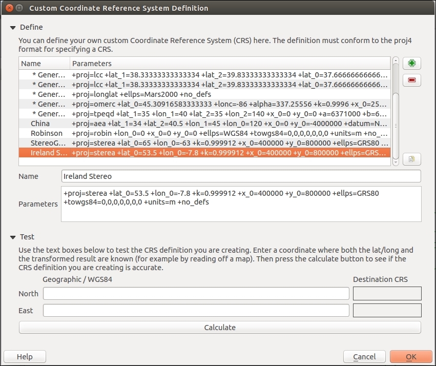
- Click on the + symbol to add a new definition.
- Put in a name and paste in your projection string, modifying it in this case with coordinates that center on Ireland. Change the values for the
lat_0andlon_0parameters to match the following example. This particular type of projection only takes one reference point. For projections with multiple standard parallels and meridians, you will see the number after the underscore increment:+proj=sterea +lat_0=53.5 +lon_0=-7.8 +k=0.999912 +x_0=400000 +y_0=800000 +ellps=GRS80 +towgs84=0,0,0,0,0,0,0 +units=m +no_defs
The following screenshot shows what the screen will look like:
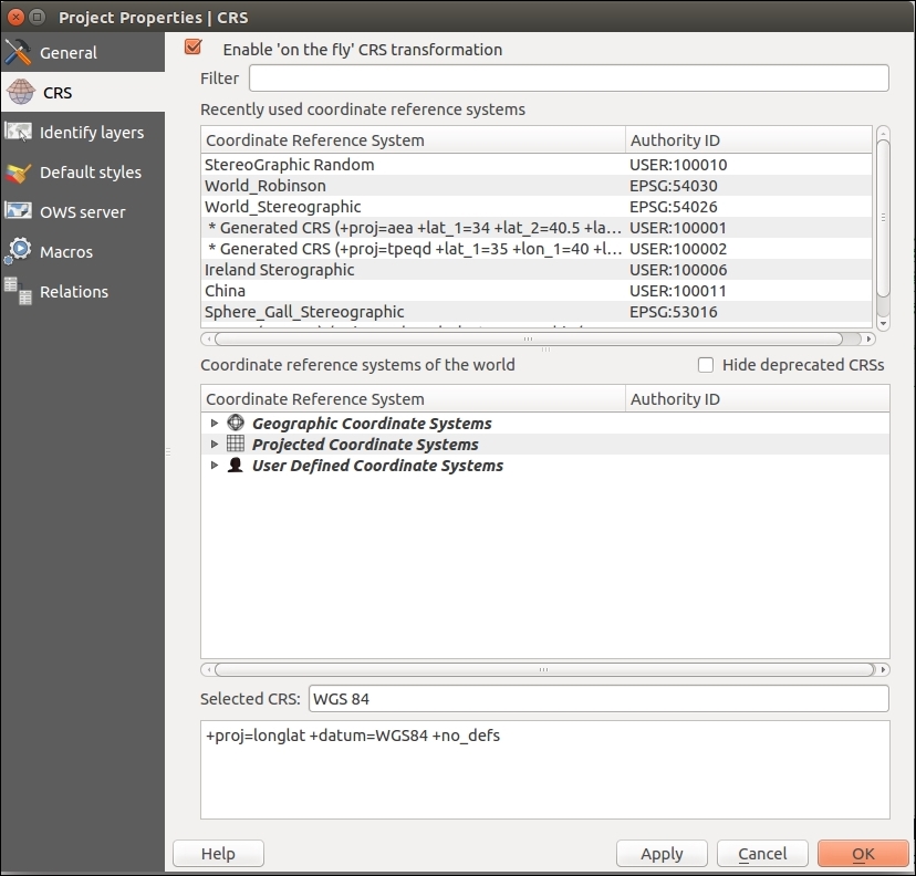
- Now, click on another projection in the list of custom projections. There's currently a quirk where if you don't toggle off to another projection, then it doesn't save when you click on OK.
- Now, go to the map, open the projection manager and apply your new projection with OTF on to check whether it's right. You'll find your new projection in the third section, User Defined Coordinate Systems:
The following screenshot shows the projection:
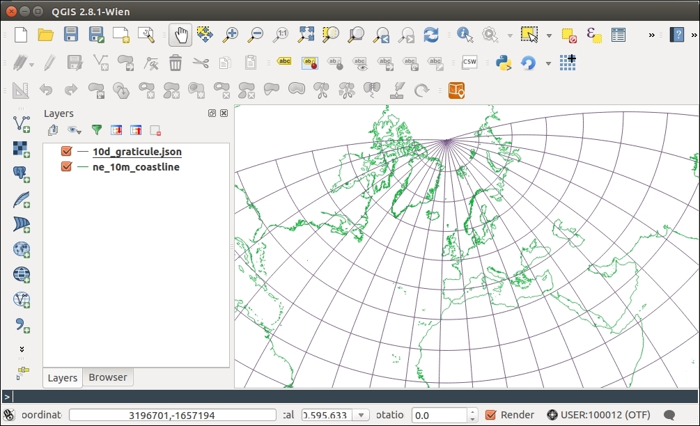
Projection information (in this case, a proj4 string) encodes the parameters that are needed by the computer to pick the correct math formula (projection type) and variables (various parameters, such as parallels and the center line) to convert the data into the desired flat map from whatever it currently is. This library of information includes approximations for the shape of the earth and differing manners to squash this into a flat visual.
You can really alter most of the parameters to change your map appearance, but generally, stick to known definitions so that your map matches other maps that are made the same way.
QGIS only allows forward/backward transformation projections. Cartographic forward-only projections (for example, Natural Earth, Winkel Tripel (III), and Van der Grinten) aren't in the projection list currently; this is because these reprojections are not a pure math formula, but an approximate mapping from one to the other, and the inverse doesn't always exist. You can get around this by reprojecting your data with the ogr2ogr and gdal_transform command line to the desired projection, and then loading it into QGIS with Projection-on-the-fly disabled. While the proj4 strings exist for these projections, QGIS will reject them if you try to enter them.
Geometries that cross the outer edge of projections don't always cut off nicely. You will often see this as an unexpected polygon band across your map. The easiest thing to do in this case is to remove data that is outside your intended mapping region. You can use a clip function or simply select what you want to keep and Save Selection As a new layer.
There are other common projection description formats (prj, WKT, and proj4) out there. Luckily, several websites help you translate. There are a couple of good websites to look up the existing Proj4 style projection information available at http://spatialreference.org and http://epsg.io.
- Need more information on how to pick an appropriate projection for the type of map you are making? Refer to the USGS classic map projections poster available at http://egsc.usgs.gov/isb/pubs/MapProjections/projections.html. Much of this is also used in the Wikipedia article on the topic available at http://en.wikipedia.org/wiki/Map_projection. The https://www.mapthematics.com/ProjectionsList.php link also has a great list of projections, including unusual ones with pictures.