Interpolated model values

In this section, we will cover the creation of new statewide, point-based vulnerability index data from our limited weather station data obtained from the MySQL database mentioned before.

Python for workflow automation

With Python's large and growing number of wrappers, which allow independent (often C written and compiled) libraries to be called directly into Python, it is the natural choice to communicate with other software. Apart from direct API and library use, Python also provides access to system automation tasks.

Knowing your environment

A deceptively simple challenge in developing with Python is of knowing which paths and dependencies are loaded into your development environment.

To print your paths, type out the following in the QGIS Python Console (navigate to Plugins | Python Console) or the OSGeo4W Shell bundled with QGIS:

import os
try:
  user_paths = os.environ['PYTHONPATH'].split(os.pathsep)
except KeyError:
  user_paths = []
print user_paths

To list all the modules so that we know which are already available, type out the following:

import sys
sys.modules.keys()

Once we know which modules are available to Python, we can look up documentation on those modules and the programmable objects that they may expose.

Tip

Remember to view all the special characters (including whitespace) in whatever text editor or IDE you are using. Python is sensitive to indentation as it relates to code blocks! You can set your text editor to automatically write the tabs as a default number of spaces. For example, when I hit a tab to indent, I will get four spaces instead of a special tab character.

Generating the parameter grids for each time period

Now, we're going to move into nonevaluation code. You may want to take this time to quit QGIS, particularly if you've been working in the Python command pane. If I'm already working on the command pane, I like to quit using Python syntax with the following code:

quit()

After quitting, start QGIS up again. The Python Console can be found under Plugins | Python Console.

By running the next code snippet in Python, you will generate a command-line code, which we will run, in turn, to generate intermediate data for this web application.

What this code does

We will run a Python code to generate a more verbose script that will perform a lengthy workflow process.

For each parameter (factor), it will loop through every day in the range of days. The range will effectively be limited to 06/10/15 through 06/30/15 as the model requires a 10-day retrospective period.
We will run it via ogr2ogr—GDAL's powerful vector data transformation tool—and use the SQLite syntax, selecting the appropriate aggregate value (count, sum, and average) based on the relative period.
It will translate each result by the threshold to scores for our calculation of vulnerability to mildew. In other words, using some (potentially arbitrary) breaks in the data, we will translate the real measurements to smaller integer scores related to our study.
It will interpolate the scores as an integer grid.

Running a code in Python

Copy and paste the following lines into the Python interpreter. Press Enter if the code is pasted without execution. The code also assumes that data can be found in the locations hardcoded in the following (C:/packt/c6/data/prep/ogr.sqlite). You may need to move these files if they are not already in the given locations or change the code. You will also need to modify the following code according to your filesystem; Windows filesystem conventions are used in the following code:

# first variable to store commands
strCmds = 'del /F C:\packt\c6\data\prep\ogr.* \n'
# list of factors
factors = ['temperature','relative_humidity','precipitation']
# iterate through each factor, appending commands for each
for factor in factors:
  for i in range(10, 31):
    j = i - 5
    k = i - 9
    if factor == 'temperature':
      # commands use ogr2ogr executable from gdal project
      # you can run help on this from command line for more
      # information on syntax
        strOgr = 'ogr2ogr -f sqlite -sql "SELECT div_field_, GEOMETRY, AVG(o_value) AS o_value FROM (SELECT div_field_, GEOMETRY, MAX(value) AS o_value, date(time_measu) as date_f FROM {2} WHERE date_f BETWEEN date(\'2013-06-{0:02d}\') AND date(\'2013-06-{1:02d}\') GROUP BY div_field_, date(time_measu)) GROUP BY div_field_" -dialect sqlite -nln ogr -dsco SPATIALITE=yes -lco SPATIAL_INDEX=yes -overwrite C:/packt/c6/data/prep/ogr.sqlite C:/packt/c6/data/prep/temperature.shp \n'.format(j,i,factor)
        strOgr += 'ogr2ogr -sql "UPDATE ogr SET o_value = 0 WHERE o_value <=15.55" -dialect sqlite -update C:/packt/c6/data/prep/ogr.sqlite C:/packt/c6/data/prep/ogr.sqlite \n'
        strOgr += 'ogr2ogr -sql "UPDATE ogr SET o_value = 3 WHERE o_value > 25.55" -dialect sqlite -update C:/packt/c6/data/prep/ogr.sqlite C:/packt/c6/data/prep/ogr.sqlite \n'
        strOgr += 'ogr2ogr -sql "UPDATE ogr SET o_value = 2 WHERE o_value > 20.55 AND o_value <= 25.55" -dialect sqlite -update C:/packt/c6/data/prep/ogr.sqlite C:/packt/c6/data/prep/ogr.sqlite \n'
        strOgr += 'ogr2ogr -sql "UPDATE ogr SET o_value = 1 WHERE o_value > 15.55 AND o_value <= 20.55" -dialect sqlite -update C:/packt/c6/data/prep/ogr.sqlite C:/packt/c6/data/prep/ogr.sqlite \n'
        elif factor == 'relative_humidity':
        strOgr = 'ogr2ogr -f sqlite -sql "SELECT GEOMETRY, COUNT(value) AS o_value, date(time_measu) as date_f FROM relative_humidity WHERE value > 96 AND date_f BETWEEN date(\'2013-06-{0:02d}\') AND date(\'2013-06-{1:02d}\') GROUP BY div_field_" -dialect sqlite -nln ogr -dsco SPATIALITE=yes -lco SPATIAL_INDEX=yes -overwrite C:/packt/c6/data/prep/ogr.sqlite C:/packt/c6/data/prep/relative_humidity.shp \n'.format(j,i)
        strOgr += 'ogr2ogr -sql "UPDATE ogr SET o_value = 0 WHERE o_value <= 1" -dialect sqlite -update C:/packt/c6/data/prep/ogr.sqlite C:/packt/c6/data/prep/ogr.sqlite \n'
        strOgr += 'ogr2ogr -sql "UPDATE ogr SET o_value = 3 WHERE o_value > 40" -dialect sqlite -update C:/packt/c6/data/prep/ogr.sqlite C:/packt/c6/data/prep/ogr.sqlite \n'
        strOgr += 'ogr2ogr -sql "UPDATE ogr SET o_value = 2 WHERE o_value > 20 AND o_value <= 40" -dialect sqlite -update C:/packt/c6/data/prep/ogr.sqlite C:/packt/c6/data/prep/ogr.sqlite \n'
        strOgr += 'ogr2ogr -sql "UPDATE ogr SET o_value = 1 WHERE o_value > 10 AND o_value <= 20" -dialect sqlite -update C:/packt/c6/data/prep/ogr.sqlite C:/packt/c6/data/prep/ogr.sqlite \n'
        strOgr += 'ogr2ogr -sql "UPDATE ogr SET o_value = 1 WHERE o_value > 1 AND o_value <= 10" -dialect sqlite -update C:/packt/c6/data/prep/ogr.sqlite C:/packt/c6/data/prep/ogr.sqlite \n'
        elif factor == 'precipitation':
        strOgr = 'ogr2ogr  -f sqlite -sql "SELECT GEOMETRY, SUM(value) AS o_value, date(time_measu) as date_f FROM precipitation WHERE date_f BETWEEN date(\'2013-06-{0:02d}\') AND date(\'2013-06-{1:02d}\') GROUP BY div_field_" -dialect sqlite -nln ogr -dsco SPATIALITE=yes -lco SPATIAL_INDEX=yes -overwrite C:/packt/c6/data/prep/ogr.sqlite C:/packt/c6/data/prep/precipitation.shp \n'.format(k,i)
        strOgr += 'ogr2ogr -sql "UPDATE ogr SET o_value = 0 WHERE o_value < 25.4" -dialect sqlite -update C:/packt/c6/data/prep/ogr.sqlite C:/packt/c6/data/prep/ogr.sqlite \n'
        strOgr += 'ogr2ogr -sql "UPDATE ogr SET o_value = 3 WHERE o_value > 76.2" -dialect sqlite -update C:/packt/c6/data/prep/ogr.sqlite C:/packt/c6/data/prep/ogr.sqlite \n'
        strOgr += 'ogr2ogr -sql "UPDATE ogr SET o_value = 2 WHERE o_value > 50.8 AND o_value <= 76.2" -dialect sqlite -update C:/packt/c6/data/prep/ogr.sqlite C:/packt/c6/data/prep/ogr.sqlite \n'
        strOgr += 'ogr2ogr -sql "UPDATE ogr SET o_value = 1 WHERE o_value > 30.48 AND o_value <= 50.8" -dialect sqlite -update C:/packt/c6/data/prep/ogr.sqlite C:/packt/c6/data/prep/ogr.sqlite \n'
        strOgr += 'ogr2ogr -sql "UPDATE ogr SET o_value = 1 WHERE o_value > 25.4 AND o_value <= 30.48" -dialect sqlite -update C:/packt/c6/data/prep/ogr.sqlite C:/packt/c6/data/prep/ogr.sqlite \n'
        strGrid = 'gdal_grid -ot UInt16 -zfield o_value -l ogr -of GTiff C:/packt/c6/data/prep/ogr.sqlite C:/packt/c6/data/prep/{0}Inter{1}.tif'.format(factor,i)
        strCmds = strCmds + strOgr + '\n' + strGrid + '\n' + 'del /F C:\packt\c6\data\prep\ogr.*' + '\n'

print strCmds

Running the printed commands in the Windows command console

Run the code output from the previous section by copying and pasting the result in the Windows command console. You can also find the output of the code to copy in c6/data/output/generate_values.bat.

The subprocess module

The subprocess module allows you to open up any executable on your system using the relevant command line syntax.

Although we could alternatively direct the code that we just produced through the subprocess module, it is simpler to do so directly on the command line in this case. With shorter, less sequential processes, you should definitely go ahead and use subprocess.

To use subprocess, just import it (ideally) in the beginning of your program and then use the Popen method to call your command line code. Execute the following code:

import subprocess
...
subprocess.Popen(strCmds)

Calculating the vulnerability index

GDAL_CALC evaluates an algebraic expression with gridded data as variables. In other words, you can use this GDAL utility to run map algebra or raster calculator type expressions. Here, we will use GDAL_CALC to produce our grid of the vulnerability index values based on the interpolated threshold scores.

Open a Python Console in QGIS (navigate to Plugins | Python Console) and copy/paste/run the following code. Again, you may wish to quit Python (using quit()) and restart QGIS/Python before running this code, which will produce the intermediate data for our application. This is used to control the unexpected variables and imported modules that are held back in the Python session.

After you've pasted the following lines into the Python interpreter, press Enter if it has not been executed. This code, like the previous one, produces a script that includes a range of numbers attached to filenames. It will run a map algebra expression through gdal_calc using the respective number in the range. Execute the following:

strCmd = ''

for i in range(10, 31):
  j = i - 5
  k = i - 9
  strOgr = 'gdal_calc --A C:/packt/c6/data/prep//temperatureInter{0}.tif -B C:/packt/c6/data/prep/relative_humidityInter{0}.tif -C C:/packt/c6/data/prep/precipitationInter{0}.tif --calc="A+B+C" --type=UInt16 --outfile=C:/packt/c6/data/prep/calc{0}.tiff'.format(i)

  strCmd += strOgr + '\n'

print strCmd

Now, run the output from this code in the Windows command console. You can find the output code under c6/data/output/calculate_index.bat.

Creating regular points

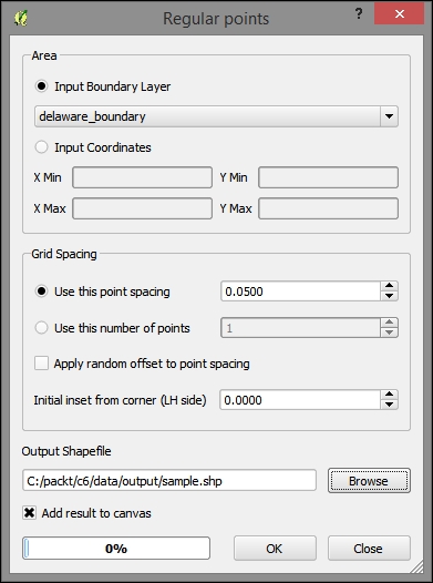
As dynamic web map interfaces are not usually good at querying raster inputs, we will create an intermediate set of locations—points—to use for interaction with a user click event. The Regular points tool will create a set of points at a regular distance from each other. The end result is almost like a grid but made up of points. Perform the following steps:

Add c6/data/original/delaware_boundary.shp to your map project if you haven't already done so.
In Vector, navigate to Research Tools | Regular points.
Use delaware_boundary for the Input Boundary Layer.
Use a point spacing of .05 (in decimal degrees for now).
Save under c6/data/output/sample.shp.

The following image shows these parameters populated:

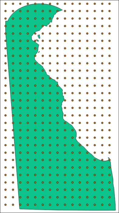
The output will look similar to this:

Sampling the index grid by points

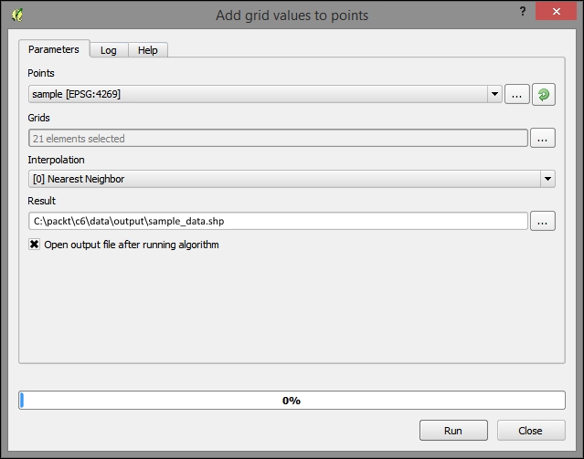
Now that we have regular points, we can attach the grid values to them using the following steps:

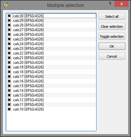
Add all the calculated grids to the map (calc10 to calc30) if they were not already added (navigate to Layer | Add Layer | Add Vector Layer).
Search for points under the Processing Toolbox pane. Ensure that the Advanced Interface is selected from the dropdown at the bottom of the pane.
Navigate to SAGA | Shapes - Grid | Add grid values to points.
Select the sample layer of regular points, which we just created. Following is a screenshot of this, and you will need to execute the following code:
```
Select all grids (calc10-calc30)
```
Save the output result to c6/data/output/sample_data.shp.
Click on Run, as shown in the following screenshot:

Create SQLite database and import

Next, create a SpatiaLite database at c6/data/web/cgi-bin/c6.sqlite (refer to the Creating a SpatiaLite database section of Chapter 5, Demonstrating Change) and import the sample_data shapefile using DB Manager.

DB Manager does not "see" SpatiaLite databases which were not created directly by the Add Layer command (as we've done so far; for example, in Chapter 5, Demonstrating Change), so it is best to do it this way rather than by saving it directly as a SpatiaLite database using the output dialog in the previous step.

Perform the following steps to test that our nearest neighbor result is correct:

Use the coordinate capture to get a test coordinate based on the points in the sample_data layer.
Create a SpatiaLite database using steps from Chapter 5, Demonstrating Change (navigate to Layer | Create Layer).
Open DB Manager (Database | DB Manager).
Import the sample_data layer/shapefile.
Run the following query in the DB Manager SQL window, substituting the coordinates that you obtained in step 1, separated by a space (for example, 75.28075 39.47785):
```
SELECT pk, calc10, min(Distance(PointFromText('POINT (-75.28075 39.47785)'),geom)) FROM vulnerability
```