In this section, we'll take a look at how to change the time settings for packets and troubleshooting with the time column.

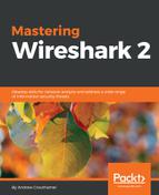
We have the PBS packet capture again, where I opened the browser and went to http://www.pbs.org/. If you notice in the packet capture, the second column says Time:

The Time column is a number with a decimal and it just keeps counting up as you scroll down through the packet capture. By default, in Wireshark, this is the time since the capture started. Having the time since it was captured can be useful so you know when certain packets arrive in relation to the entire data flow that you captured, but it's not all that useful for trying to diagnose a problem where there might be a delay in a certain service returning traffic that you're trying to capture back to your system.

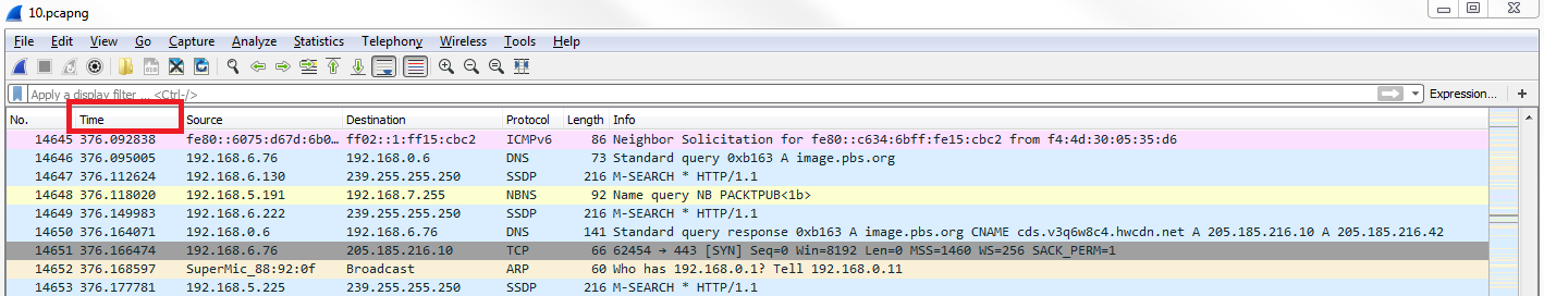
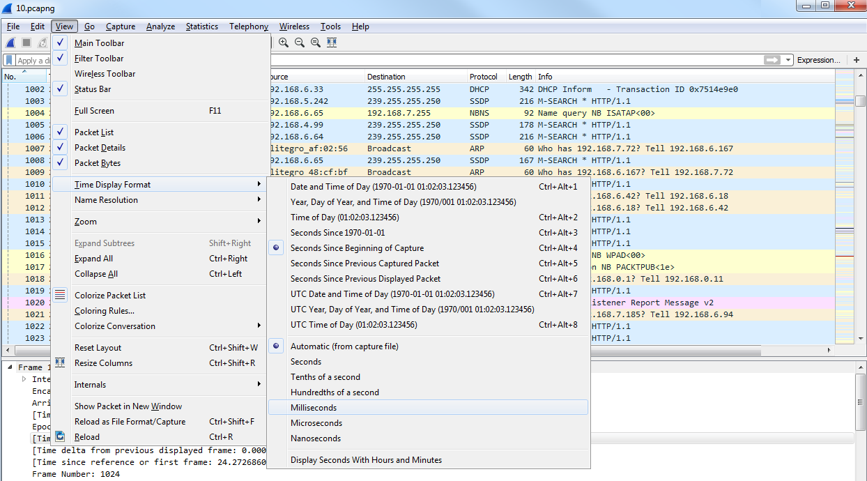
In order to figure out the delay between captured packets, you'd have to look at the Time column and figure it out based on milliseconds, microseconds, and nanoseconds, and that's not that great for humans because we're not all that great at math to that level. So what we can do instead is go to View | Time Display Format, and we have a large selection of time display formats we can choose from. And the most useful one that I would recommend is using Seconds Since Previous Displayed Packet:

This way, if you apply a filter on your traffic, such as following a TCP stream, it will show you the delta difference between each packet based on the applied filter. If you use Seconds Since Previous Captured Packet, then if you have packets that are filtered out from the view that you're looking at, it'll not coincide exactly with what you're looking at; it makes it a little bit harder to understand. So what I would recommend is choosing Seconds Since Previous Displayed Packet.

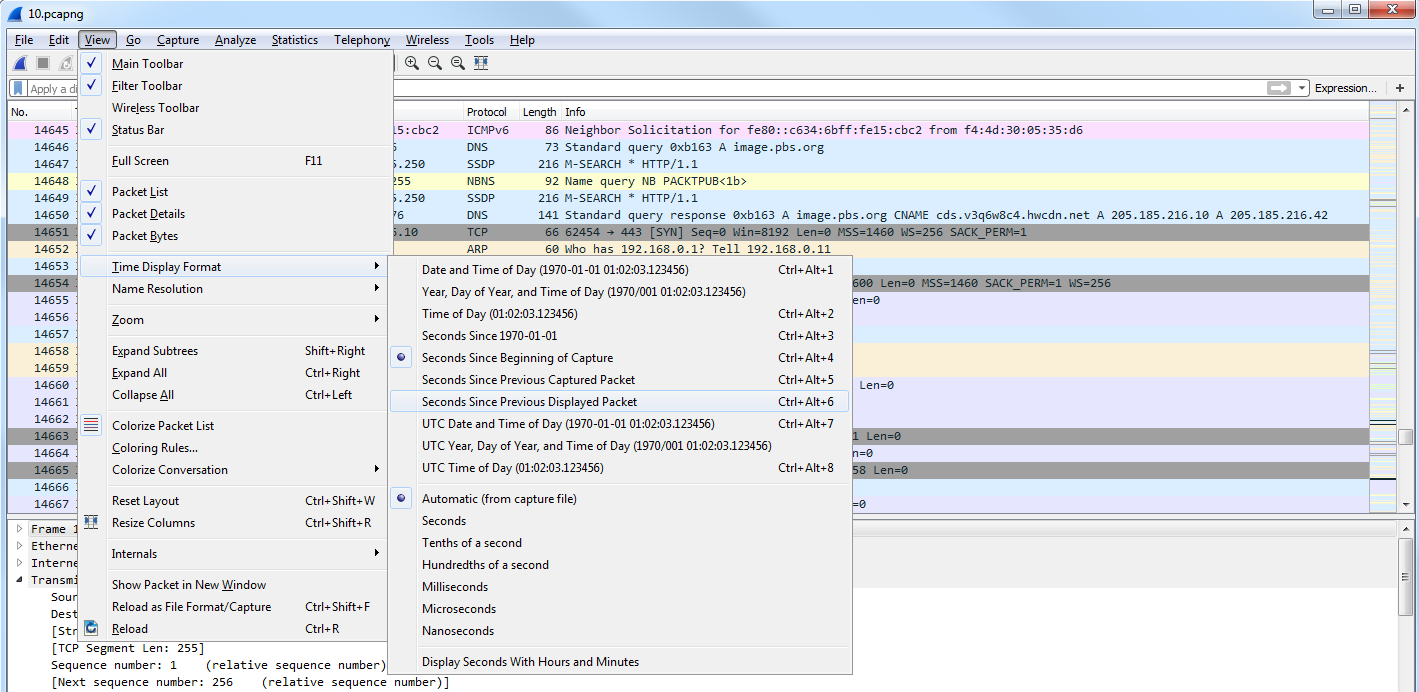
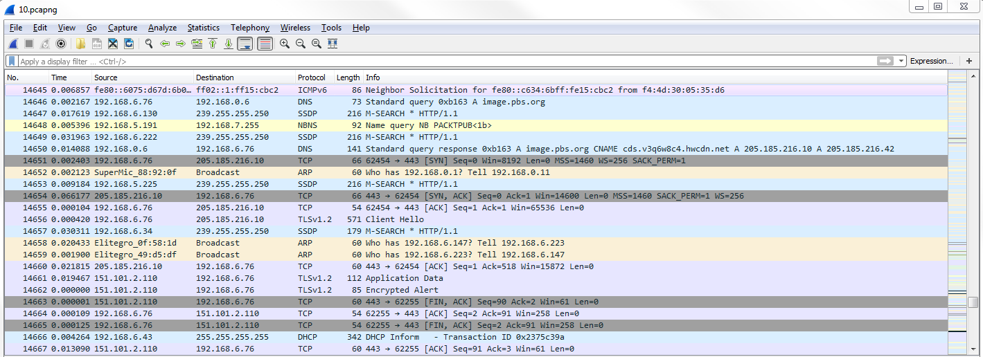
Now if we look, the Time column has changed and we have 0 seconds between each packet, and then there's some sort of fraction of a second for each packet for the delay between each captured packet:

What we'll do is we'll scroll up to the top and you can sort the Time column. And if you sort it by highest to lowest, you can see what packets are the most delayed. Now, if you select that packet and then re-sort by the No. column, you'll be taken directly to that packet, wherever it is within the numbered packets that you've captured. You can look on either side of the packet to figure out what might be going on.

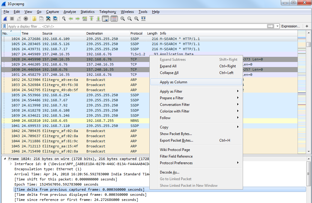
You can also add additional columns. So, what we can do is go to packet details and expand the frame information. And you'll see there are a number of time fields. What we can do is also add a column for one of these time fields. So, what we'll do first is we'll switch our display back to since the beginning of the capture by going to View | Time Display Format format | Seconds Since Begining of Capture, and we'll add a column for the delta between each displayed frame. We'll do that by selecting Time delta from previous captured frame from the frame information. We'll right-click and select Apply as Column:

Then, we drag the Time delta from previous displayed frame column over to the other time so that it makes it a little bit easier.

So, you have time since the capture began, and then time delta between each displayed frame. You can also go to View | Time Display Format and change the fraction of seconds based on what you want to see. So, maybe you don't need to see the nanoseconds, and you only care about the milliseconds. You can change that manually by selecting the Milliseconds option: 

You will now be able to see how it pruned our Time column.

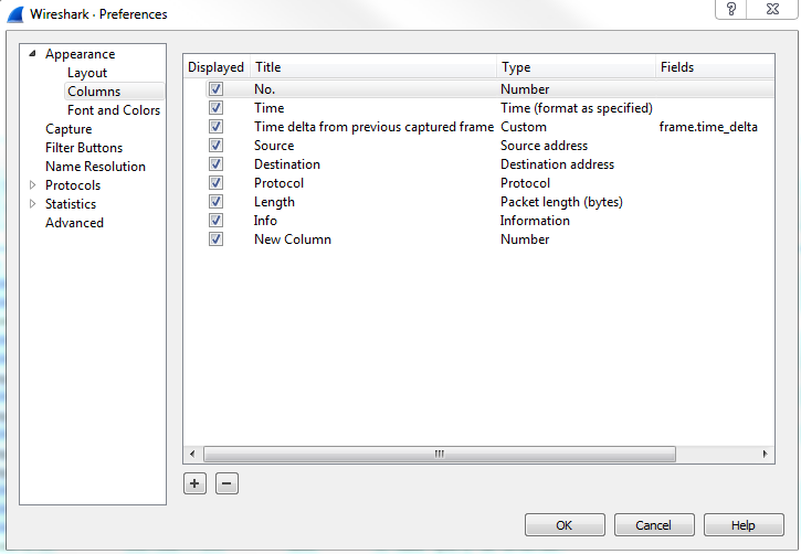
You can also add columns by going to Edit | Preferences... and then to the Appearance | Columns area, and you can manually add whatever column you want by clicking on the plus sign:

Lastly, if you go to Statistics | Capture File Properties, you'll see a list of information based on the packet capture. And if you scroll down, you'll notice that there's a whole bunch of statistics on the capture itself, including the number of packets, the time span, how big this packet capture is in number of seconds, average packets per second, average byte size, total number of bytes that have been captured, average bytes per second, and average bits per second:

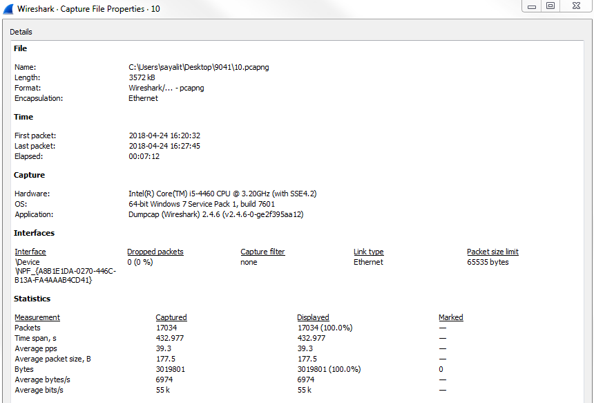
This summary can be useful when comparing a capture done during a benchmark, when everything is running normally, and compared to a packet capture performed when there are performance issues. You can see if there are any of these values in the summary statistics that have changed drastically.