Table of Contents for

Your Code as a Crime Scene

Predict Defects

A high degree of code churn isn’t a problem in and of itself. It’s more of a symptom, because code changes for a reason. Perhaps we have a feature area that’s poorly understood. Or maybe we just have a module with a low-quality implementation.

Given these reasons, it’s hardly surprising that code churn is a good predictor of defects. Let’s see how we can use that in our hotspot analyses.

Analyze Churn on an Architectural Level

In Chapter 10, ​Use Beauty as a Guiding Principle​, we used temporal coupling to identify expensive change patterns in different architectures. We used the analysis results to detect modification patterns that violated architectural principles. Code churn measures supplement such analyses as well. Let’s see how. In the architectural analyses, we specify a transformation file. This file defines our architecturally significant components. To run a churn analysis on that level, we just specify the same transformation when we request an entity-churn analysis. When combined with temporal coupling, code churn provides additional insights on how serious the identified dependencies are.

Detect Hotspots by Churn

In this book, we used the number of revisions of each module to detect hotspots. It’s a simple metric that works surprisingly well. But it sure has its limitations. (We discussed them back in ​Limitations of the Hotspot Criteria​.)

Code churn gives you an alternative metric that avoids some of these biases. Here are the typical cases where you should consider code churn:

• Differences in individual commit styles: Some developers keep their commits small and cohesive; others stick to big-bang commits.

• Long-lived feature branches: If we develop code on branches that live for weeks without being merged, as you see in the following figure, we may lose important history with regard to the original change frequencies on the branch.

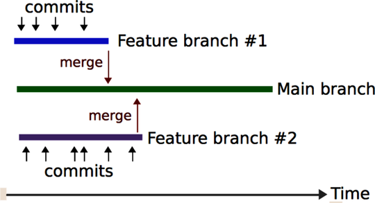
While both scenarios indicate symptoms of deeper problems, sometimes you’ll find yourself in one of them. In that case, code churn provides a more accurate metric than raw change frequencies.

To use code churn in a hotspot analysis, you combine the results from an entity-churn analysis with a complexity metric—for example, lines of code. The overlap between these two dimensions lets you identify the hotspots.

Consider Relative Code Churn

The code churn measures we’ve used so far are based on absolute churn values. That means code churn erases the differences between commit styles; it no longer matters if someone puts a day’s work into a single commit or if you commit often. All that matters is the amount of code that was affected.

However, it’s worthwhile to investigate an alternative measure. In Use of relative code churn measures to predict system defect density [NB05], a research team found that code churn was highly predictive of bugs. The twist is that the researchers used a different measure than we do. They measured relative code churn.

Relative code churn means that the absolute churn values are adjusted by the size of each file. And according to that research paper, the relative churn values outperform measures of absolute churn. So, have I wasted your time with almost a whole chapter devoted to absolute churn? I certainly hope not. Let’s see why.

First of all, a subsequent research paper found no difference between the effectiveness of absolute and relative churn measures. In fact, absolute values proved to be slightly better at predicting defects. (See Does Measuring Code Change Improve Fault Prediction? [BOW11].) Further, relative churn values are more expensive to calculate. You need to iterate over past revisions of each file and calculate the total amount of code. Compare that to just parsing a version-control log, as we do to get absolute churn values.

The conclusion is that we just cannot tell for sure whether one measure is better than the other. It may well turn out that different development styles and organizations lend themselves better to different measures. In the meantime, I recommend that you start with absolute churn values. Simplicity tends to win in the long run.

Know the Limitations of Code Churn

Like all metrics, code churn has its limitations, too. You saw one such case in ​Measure the Churn Trend​, where a commit of static test data biased the results. Thus, you should be aware of the following pitfalls:

• Generated code: This problem is quite easy to solve by filtering out generated code from the analysis results.

• Refactoring: Refactorings are done in small, predictable increments. As a side effect, code that undergoes refactorings may be flagged as high churn even though we’re making it better.

• Superficial changes: Code churn is sensitive to superficial changes, such as renaming the instance variables in a class or rearranging the functions in a module.

In this chapter, we’ve used code churn to complement other analyses. We used the combined results to support and guide us. In my experience, that’s where churn measures are the most valuable. This strategy also lets you minimize the impact of code churn’s limitations.