Table of Contents for
Your Code as a Crime Scene
 Your Code as a Crime Scene
Published by
Pragmatic Bookshelf, 2015
Your Code as a Crime Scene
Published by
Pragmatic Bookshelf, 2015
- Title Page
- Your Code as a Crime Scene
- Your Code as a Crime Scene
- For the Best Reading Experience...
- Table of Contents
- Early praise for Your Code as a Crime Scene
- Foreword by Michael Feathers
- Acknowledgments
- Chapter 1: Welcome!
- About This Book
- Optimize for Understanding
- How to Read This Book
- Toward a New Approach
- Get Your Investigative Tools
- Part 1: Evolving Software
- Chapter 2: Code as a Crime Scene
- Meet the Problems of Scale
- Get a Crash Course in Offender Profiling
- Profiling the Ripper
- Apply Geographical Offender Profiling to Code
- Learn from the Spatial Movement of Programmers
- Find Your Own Hotspots
- Chapter 3: Creating an Offender Profile
- Mining Evolutionary Data
- Automated Mining with Code Maat
- Add the Complexity Dimension
- Merge Complexity and Effort
- Limitations of the Hotspot Criteria
- Use Hotspots as a Guide
- Dig Deeper
- Chapter 4: Analyze Hotspots in Large-Scale Systems
- Analyze a Large Codebase
- Visualize Hotspots
- Explore the Visualization
- Study the Distribution of Hotspots
- Differentiate Between True Problems and False Positives
- Chapter 5: Judge Hotspots with the Power of Names
- Know the Cognitive Advantages of Good Names
- Investigate a Hotspot by Its Name
- Understand the Limitations of Heuristics
- Chapter 6: Calculate Complexity Trends from Your Code’s Shape
- Complexity by the Visual Shape of Programs
- Learn About the Negative Space in Code
- Analyze Complexity Trends in Hotspots
- Evaluate the Growth Patterns
- From Individual Hotspots to Architectures
- Part 2: Dissect Your Architecture
- Chapter 7: Treat Your Code As a Cooperative Witness
- Know How Your Brain Deceives You
- Learn the Modus Operandi of a Code Change
- Use Temporal Coupling to Reduce Bias
- Prepare to Analyze Temporal Coupling
- Chapter 8: Detect Architectural Decay
- Support Your Redesigns with Data
- Analyze Temporal Coupling
- Catch Architectural Decay
- React to Structural Trends
- Scale to System Architectures
- Chapter 9: Build a Safety Net for Your Architecture
- Know What’s in an Architecture
- Analyze the Evolution on a System Level
- Differentiate Between the Level of Tests
- Create a Safety Net for Your Automated Tests
- Know the Costs of Automation Gone Wrong
- Chapter 10: Use Beauty as a Guiding Principle
- Learn Why Attractiveness Matters
- Write Beautiful Code
- Avoid Surprises in Your Architecture
- Analyze Layered Architectures
- Find Surprising Change Patterns
- Expand Your Analyses
- Part 3: Master the Social Aspects of Code
- Chapter 11: Norms, Groups, and False Serial Killers
- Learn Why the Right People Don’t Speak Up
- Understand Pluralistic Ignorance
- Witness Groupthink in Action
- Discover Your Team’s Modus Operandi
- Mine Organizational Metrics from Code
- Chapter 12: Discover Organizational Metrics in Your Codebase
- Let’s Work in the Communication Business
- Find the Social Problems of Scale
- Measure Temporal Coupling over Organizational Boundaries
- Evaluate Communication Costs
- Take It Step by Step
- Chapter 13: Build a Knowledge Map of Your System
- Know Your Knowledge Distribution
- Grow Your Mental Maps
- Investigate Knowledge in the Scala Repository
- Visualize Knowledge Loss
- Get More Details with Code Churn
- Chapter 14: Dive Deeper with Code Churn
- Cure the Disease, Not the Symptoms
- Discover Your Process Loss from Code
- Investigate the Disposal Sites of Killers and Code
- Predict Defects
- Time to Move On
- Chapter 15: Toward the Future
- Let Your Questions Guide Your Analysis
- Take Other Approaches
- Let’s Look into the Future
- Write to Evolve
- Appendix 1: Refactoring Hotspots
- Refactor Guided by Names
- Bibliography
- You May Be Interested In…
Analyze Temporal Coupling
In Chapter 7, Treat Your Code As a Cooperative Witness, we said that temporal coupling can be an interview tool for your codebase. The first step in an interview is to know who you should talk to.
Let’s use sum of coupling analysis to find our first code witness.
Use Sum of Coupling to Identify the Modules to Inspect
You’ve already seen that there are different reasons for modules to be coupled. Some couples, such as a unit and its unit test, are valid. So modules with the highest degree of coupling may not be the most interesting to us. Instead, we want modules that are architecturally significant. A sum of coupling analysis finds those modules.
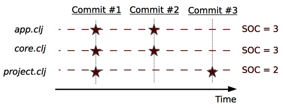
Sum of coupling looks at how many times each module has been coupled to another one in a commit and sums it up. For example, in the following figure, you see that module app.clj changed with both core.clj and project.clj in Commit #1, but just with core.clj in Commit #2. Its sum of coupling is three.
The module that changes most frequently together with others must be important and is a good starting point for an investigation. Let’s try it out on Code Maat by reusing the the logfile we mined in Chapter 3, Creating an Offender Profile.
Move into the top-level directory in your Code Maat repository and type the following command:
| | prompt> maat -l maat_evo.log -c git -a soc |
| | entity,soc |
| | src/code_maat/app/app.clj,105 |
| | test/code_maat/end_to_end/scenario_tests.clj,97 |
| | src/code_maat/core.clj,93 |
| | project.clj,74 |
| | ... |
You can see that this command uses the same format we saw in the earlier hotspot analysis. The only difference is that we’re requesting -a soc (sum of coupling) instead.
We see that app.clj changes the most with other modules. Let’s keep an eye on app.clj as we dive deeper.
Measure Temporal Coupling
At this point you know that app.clj is the module with the most temporal coupling. The next step is to find out which modules it’s coupled to. We use Code Maat for this analysis:
| | prompt> maat -l maat_evo.log -c git -a coupling |
| | entity,coupled,degree,average-revs |
| | src/code_maat/parsers/git.clj,test/code_maat/parsers/git_test.clj,83,12 |
| | src/code_maat/analysis/entities.clj,test/code_maat/analysis/entities_test.clj,76,7 |
| | src/code_maat/analysis/authors.clj,test/code_maat/analysis/authors_test.clj,72,11 |
| | ... |
The command line is identical to the one you just used, with the exception that we’re requesting -a coupling instead. The resulting CSV output contains plenty of information:
-
entity: This is the name of one of the involved modules. Code Maat always calculates pairs.
-
coupled: This is the coupled counterpart to the entity.
-
degree: The degree specifies the percent of shared commits. The higher the number, the stronger the coupling. For example, git.clj and git_test.clj change together in 83 percent of all commits.
-
average-revs: Finally, we get a weighted number of total revisions for the involved modules. The idea here is that we can filter out modules with too few revisions to avoid bias.
You see a typical pattern in the output: each unit changes together with its unit test (e.g. git.clj and git_test.clj, entities.clj and entities_test.clj).
This kind of temporal coupling is expected and not a problem. Code Maat was developed with test-driven development, so I’d say that getting any other result would’ve been a problem. Just plain old physical coupling—nothing too exciting here.
Things get interesting a bit farther down:
| | prompt> maat -l maat_evo.log -c git -a coupling |
| | ... |
| | src/code_maat/app/app.clj,src/code_maat/core.clj,60,23 |
| | src/code_maat/app/app.clj,test/code_maat/end_to_end/scenario_tests.clj,57,23 |
| | ... |
We see that app.clj changed with core.clj 60 percent of the time and with scenario_tests.clj 57 percent of the time. There’s no way to tell why just from the names alone, but 60 percent is a high degree of coupling. We are talking about every second (or so), change in app.clj triggering a change in two other modules. That can’t be good. Let’s investigate why.
Check Out the Evolution Radar | |
|---|---|
|
|
In a large codebase, a temporal coupling analysis sparks an explosion of data. Code Maat resolves that by allowing us to specify optional thresholds. The research tool Evolution Radar[24] takes a different approach and lets us zoom in and out to the level of detail we’re interested in. So check out the tool and take inspiration. |
Investigate Temporal Couples
Once we make such a finding, we need to drill down into the code. Because all changes are recorded in our version-control system, we can perform a diff on the modules. I’d recommend focusing on the shared commits and look for recurring modification patterns within those commits.
Code Maat is written in Clojure. Although an exciting language, it’s far outside the scope of this book. So let’s stay with temporal coupling, and allow me to walk you through the design to spot the problems.
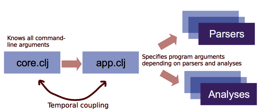
I’m a bit ashamed to admit that core.clj is the command-line interface of Code Maat. (I changed it later to a better name.) It parses the arguments you give it, converts them to a Clojure representation, and forwards them to app.clj.
app.clj glues the program together by mapping the given arguments to the correct invocations of parsers, analyses, and output formats. As you can see, the program arguments cause the coupling; every time a new argument is added, two distinct modules have to evolve to know about it.
So, your first takeaway is actually a reminder about the power of names that you learned about in Chapter 5, Judge Hotspots with the Power of Names. With proper naming, we’d have a better entry point for our manual code inspection. Second, we failed to encapsulate a concept that varies. If we extract the knowledge of all command-line arguments from app.clj, we break the coupling and make the code easier to evolve and maintain.
Use Temporal Coupling for Design Insights
The analysis on Code Maat illustrates how we can use temporal coupling analysis on small projects. Code Maat (which I wrote to learn Clojure during my daily commute) is a single-developer project with less than 2,000 lines of code.
Such small projects don’t need a hotspot analysis. We already know which modules are hard to change. Temporal coupling is different because it provides insights into our design. We get active feedback on our work so that we can spot improvements we hadn’t even thought of.
Keep Your Temporal Coupling Algorithms Simple
The algorithm we’ve used so far isn’t the only kid in town. Temporal coupling means that some entities change together over time. But there isn’t any formal definition of what change together means. In research papers, you’ll find several alternative measures.
One typical alternative adds the notion of time to the algorithm; the degree of coupling is weighted by the age of the commits. The idea is to prioritize recent changes over changes in the more distant past. A relationship thus gets weaker with the passage of time. However, as you’ll see soon when we discuss software defects, a time parameter doesn’t necessarily improve the metric.
The algorithm that Code Maat implements, the percent of shared commits, is chosen because when faced with several alternatives that seem equally good, simplicity tends to win. The Code Maat measure is straightforward to implement and, more importantly, intuitive to reason about and verify.
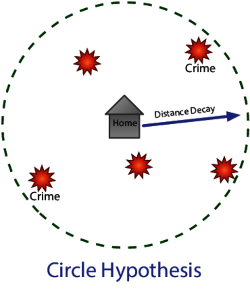
Interestingly enough, simplicity may win in criminal investigations, too. In a fascinating study, researchers trained people on two simple heuristics for predicting the home location of criminals:
|
Using these simple principles allowed the participants to predict the likely home location of serial killers with the same accuracy as a sophisticated geographical profiling system. (See Applications of Geographical Offender Profiling [CY08].) We build the techniques in this book on the same kind of simplicity.
Know the Limitations of Temporal Coupling
Our simple definition of temporal coupling as modules that change in the same commit works well. Often, that definition takes us far enough to identify unexpected relationships in our system. But in larger organizations, our measure is too narrow. When multiple teams are responsible for different parts of the system, the temporal period of interest is probably counted in days or even weeks. We’ll address this problem in Chapter 12, Discover Organizational Metrics in Your Codebase, where you’ll learn to group multiple commits into a logical change set based on a custom timespan.
Another problem with the measure is that we’re limited to the information contained in commits. We may miss important coupling relationships that occur between commits. The solution to this problem requires hooks into our text editors and our IDE to record precise information on our code interactions. Tools like that are under active research.
Yet another bias is moving and renaming modules. While version-control systems track renames, Code Maat does not. (If I ever turn Code Maat into a commercial product, that’s a feature I’d add.) It sounds more limiting than it actually is: problematic modules tend to remain where they are. The good thing is that because we lose some of the supporting information, the results we get are more likely to point to true problems. Consider renaming the module as a reset switch triggered by refactoring.