Table of Contents for
Your Code as a Crime Scene
 Your Code as a Crime Scene
Published by
Pragmatic Bookshelf, 2015
Your Code as a Crime Scene
Published by
Pragmatic Bookshelf, 2015
- Title Page
- Your Code as a Crime Scene
- Your Code as a Crime Scene
- For the Best Reading Experience...
- Table of Contents
- Early praise for Your Code as a Crime Scene
- Foreword by Michael Feathers
- Acknowledgments
- Chapter 1: Welcome!
- About This Book
- Optimize for Understanding
- How to Read This Book
- Toward a New Approach
- Get Your Investigative Tools
- Part 1: Evolving Software
- Chapter 2: Code as a Crime Scene
- Meet the Problems of Scale
- Get a Crash Course in Offender Profiling
- Profiling the Ripper
- Apply Geographical Offender Profiling to Code
- Learn from the Spatial Movement of Programmers
- Find Your Own Hotspots
- Chapter 3: Creating an Offender Profile
- Mining Evolutionary Data
- Automated Mining with Code Maat
- Add the Complexity Dimension
- Merge Complexity and Effort
- Limitations of the Hotspot Criteria
- Use Hotspots as a Guide
- Dig Deeper
- Chapter 4: Analyze Hotspots in Large-Scale Systems
- Analyze a Large Codebase
- Visualize Hotspots
- Explore the Visualization
- Study the Distribution of Hotspots
- Differentiate Between True Problems and False Positives
- Chapter 5: Judge Hotspots with the Power of Names
- Know the Cognitive Advantages of Good Names
- Investigate a Hotspot by Its Name
- Understand the Limitations of Heuristics
- Chapter 6: Calculate Complexity Trends from Your Code’s Shape
- Complexity by the Visual Shape of Programs
- Learn About the Negative Space in Code
- Analyze Complexity Trends in Hotspots
- Evaluate the Growth Patterns
- From Individual Hotspots to Architectures
- Part 2: Dissect Your Architecture
- Chapter 7: Treat Your Code As a Cooperative Witness
- Know How Your Brain Deceives You
- Learn the Modus Operandi of a Code Change
- Use Temporal Coupling to Reduce Bias
- Prepare to Analyze Temporal Coupling
- Chapter 8: Detect Architectural Decay
- Support Your Redesigns with Data
- Analyze Temporal Coupling
- Catch Architectural Decay
- React to Structural Trends
- Scale to System Architectures
- Chapter 9: Build a Safety Net for Your Architecture
- Know What’s in an Architecture
- Analyze the Evolution on a System Level
- Differentiate Between the Level of Tests
- Create a Safety Net for Your Automated Tests
- Know the Costs of Automation Gone Wrong
- Chapter 10: Use Beauty as a Guiding Principle
- Learn Why Attractiveness Matters
- Write Beautiful Code
- Avoid Surprises in Your Architecture
- Analyze Layered Architectures
- Find Surprising Change Patterns
- Expand Your Analyses
- Part 3: Master the Social Aspects of Code
- Chapter 11: Norms, Groups, and False Serial Killers
- Learn Why the Right People Don’t Speak Up
- Understand Pluralistic Ignorance
- Witness Groupthink in Action
- Discover Your Team’s Modus Operandi
- Mine Organizational Metrics from Code
- Chapter 12: Discover Organizational Metrics in Your Codebase
- Let’s Work in the Communication Business
- Find the Social Problems of Scale
- Measure Temporal Coupling over Organizational Boundaries
- Evaluate Communication Costs
- Take It Step by Step
- Chapter 13: Build a Knowledge Map of Your System
- Know Your Knowledge Distribution
- Grow Your Mental Maps
- Investigate Knowledge in the Scala Repository
- Visualize Knowledge Loss
- Get More Details with Code Churn
- Chapter 14: Dive Deeper with Code Churn
- Cure the Disease, Not the Symptoms
- Discover Your Process Loss from Code
- Investigate the Disposal Sites of Killers and Code
- Predict Defects
- Time to Move On
- Chapter 15: Toward the Future
- Let Your Questions Guide Your Analysis
- Take Other Approaches
- Let’s Look into the Future
- Write to Evolve
- Appendix 1: Refactoring Hotspots
- Refactor Guided by Names
- Bibliography
- You May Be Interested In…
Analyze Complexity Trends in Hotspots
In a healthy codebase, you can add new features with successively less effort. Unfortunately, the reverse is often true: new features add complexity to an already tricky design. Eventually, the system breaks down, and development slows to a crawl.
This phenomenon was identified and formalized by Manny Lehman[22] in a set of laws on software evolution. In his law of increasing complexity, Lehman states that “as an evolving program is continually changed, its complexity, reflecting deteriorating structure, increases unless work is done to maintain or reduce it.” (See On Understanding Laws, Evolution, and Conservation in the Large-Program Life Cycle [Leh80].)
You already know about hotspot analyses to identify these “deteriorating structures” so that you can react and reduce complexity. But how do we know if we are improving the code over time or just contributing to the grand decline? Let’s see how we uncover complexity trends in our programs.
Use Indentation to Analyze Complexity Trends
An indentation analysis is fast and simple. That means it scales to a range of revisions without eating up your precious time. Of course, you may well wonder if different indentation styles could affect the results. Let’s look into that.
This chapter has its theoretical foundations in the study Reading Beside the Lines: Indentation as a Proxy for Complexity Metric. Program Comprehension, 2008. ICPC 2008. The 16th IEEE International Conference on [HGH08]. That research evaluated indentation-based complexity in 278 projects. They found that indentation is relatively uniform and regular. Their study also suggests that deviating indentations don’t affect the results much.
The explanation is also the reason the technique works in the first place: indentation improves readability. It aligns closely with underlying coding constructs. We don’t just indent random chunks of code (unless we’re competing in the International Obfuscated C Code Contest).[23]
Similarly, it doesn’t really matter if we indent two or four spaces. However, a change in indentation style midway through the analysis could disturb your results. For example, running an auto-indent program on your codebase would wreck its history and show an incorrect complexity trend. If you are in that situation, you can’t compare revisions made before and after the change in indentation practices.
Even if individual indentation styles don’t affect the analysis results as much as we’d think, it’s still a good idea to keep a uniform style as it helps build consistency. With that sorted out, let’s move on to an actual analysis.
Focus on a Range of Revisions
You’ve already seen how to analyze a single revision. Now we want to:
-
Take a range of revisions for a specific module.
-
Calculate the indentation complexity of the module as it occurred in each revision.
-
Output the results revision by revision for further analysis.
With version-control systems, we can roll back to historical versions of our code and run complexity analyses on them. For example, in git we look at historical versions with the show command.
The receipe for a trend analysis is pretty straightforward, although it requires some interactions with the version-control system. Since this book isn’t about git or even version-control systems, we’re going to skip over the actual implementation details and just use the script already in your scripts directory. Don’t worry, I’ll walk you through the main steps to understand what’s happening so that you can perform your own analysis on your code.
Discover the Trend
In your cloned Hibernate Git repository, type the following into the command prompt (and remember to reference your own scripts path) to run git_complexity_trend.py:
| | prompt> python scripts/git_complexity_trend.py \ |
| | --start ccc087b --end 46c962e \ |
| | --file hibernate-core/src/main/java/org/hibernate/cfg/Configuration.java |
| | rev,n,total,mean,sd |
| | e75b8a7,3080,7610,2.47,1.76 |
| | 23a6280,3092,7649,2.47,1.76 |
| | 8991100,3100,7658,2.47,1.76 |
| | 8373871,3101,7658,2.47,1.76 |
| | ... |
This looks cryptic at first. What just happened is that we specified a range of revisions determined by the --start and --end flags. Their arguments represent our analysis period, as we see in the following image.
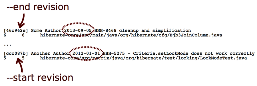
After that, you gave the name of the --file to analyze. In this case, we focus on our suspect, Configuration.java.
The analysis generates CSV output similar to the file you got during the earlier single-module analysis. The difference here is that we get the complexity statistics for each historical revision of the code. The first column specifies the commit hash from each revision’s git code. Let’s visualize the result to discover trends.
Visualize the Complexity Trend
Spreadsheets are excellent for visualizing CSV files. Just save the CSV output into a file and import it into Excel, OpenOffice, or a similar application of your choice.
Let’s look at the total complexity growth first. That would be the total column.
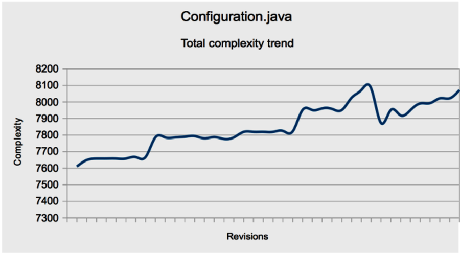
As you can see in the image, Configuration.java accumulated complexity over time.
This growth can occur in two basic ways:
-
New code is added to the module.
-
Existing code is replaced by more complex code.
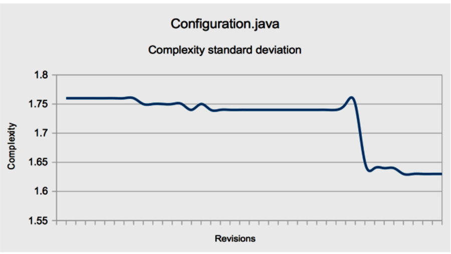
Case 2 is particularly worrisome—that’s the “deteriorating structure” Lehman’s law warned us about. We calculated the standard deviation (in the sd column) to differentiate between these two cases. Let’s see how it looks.
The standard deviation decreases. This means lines get more alike in terms of complexity, and it is probably a good thing. If you look at the mean, you see that it, too, decreases. Let’s see what that means for your programs.