Table of Contents for
Python Geospatial Development - Third Edition
 Python Geospatial Development - Third Edition
Published by
Packt Publishing, 2016
Python Geospatial Development - Third Edition
Published by
Packt Publishing, 2016
- Cover
- Table of Contents
- Python Geospatial Development Third Edition
- Python Geospatial Development Third Edition
- Credits
- About the Author
- About the Reviewer
- www.PacktPub.com
- Preface
- What you need for this book
- Who this book is for
- Conventions
- Reader feedback
- Customer support
- 1. Geospatial Development Using Python
- Geospatial development
- Applications of geospatial development
- Recent developments
- Summary
- 2. GIS
- GIS data formats
- Working with GIS data manually
- Summary
- 3. Python Libraries for Geospatial Development
- Dealing with projections
- Analyzing and manipulating Geospatial data
- Visualizing geospatial data
- Summary
- 4. Sources of Geospatial Data
- Sources of geospatial data in raster format
- Sources of other types of geospatial data
- Choosing your geospatial data source
- Summary
- 5. Working with Geospatial Data in Python
- Working with geospatial data
- Changing datums and projections
- Performing geospatial calculations
- Converting and standardizing units of geometry and distance
- Exercises
- Summary
- 6. Spatial Databases
- Spatial indexes
- Introducing PostGIS
- Setting up a database
- Using PostGIS
- Recommended best practices
- Summary
- 7. Using Python and Mapnik to Generate Maps
- Creating an example map
- Mapnik concepts
- Summary
- 8. Working with Spatial Data
- Designing and building the database
- Downloading and importing the data
- Implementing the DISTAL application
- Using DISTAL
- Summary
- 9. Improving the DISTAL Application
- Dealing with the scale problem
- Performance
- Summary
- 10. Tools for Web-based Geospatial Development
- A closer look at three specific tools and techniques
- Summary
- 11. Putting It All Together – a Complete Mapping System
- Designing the ShapeEditor
- Prerequisites
- Setting up the database
- Setting up the ShapeEditor project
- Defining the ShapeEditor's applications
- Creating the shared application
- Defining the data models
- Playing with the admin system
- Summary
- 12. ShapeEditor – Importing and Exporting Shapefiles
- Importing shapefiles
- Exporting shapefiles
- Summary
- 13. ShapeEditor – Selecting and Editing Features
- Editing features
- Adding features
- Deleting features
- Deleting shapefiles
- Using the ShapeEditor
- Further improvements and enhancements
- Summary
- Index
Our DISTAL application is certainly working, but its performance leaves something to be desired. While the selectCountry.py and selectArea.py scripts run quickly, it can take two seconds or more for the showResults.py script to complete. Clearly, this isn't good enough: a delay like this is annoying to the user but would be disastrous for the server if it started to receive more requests than it could process.
Adding some timing code to the showResults.py script soon shows where the bottleneck lies:
Calculating lat/long coordinate took 0.0110 seconds
Identifying place names took 0.0088 seconds
Generating map took 3.0208 seconds
Building HTML page took 0.0000 seconds
Clearly, the map-generation process is the problem here. Since it only took a fraction of a second to generate a map within the selectArea.py script, there's nothing inherent in the map-generation process that takes this long. So what has changed?
It could be that displaying the place names takes a while, but that's unlikely. It's far more likely to be caused by the amount of map data that we are displaying: the showResults.py script is using high-resolution shoreline outlines taken from the GSHHG dataset rather than the low-resolution country outlines taken from the World Borders Dataset. To test this theory, we can change the map data being used to generate the map, altering showResults.py to use the low-resolution countries table instead of the high-resolution shorelines table.
The result is a dramatic improvement in speed:
Generating map took 0.1729 seconds
So, how can we make the map generation in showResults.py faster? The answer lies in the nature of the shoreline data and how we are using it. Consider the situation where you are identifying points within 10 miles of Le Havre in France:
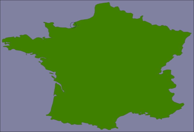
The high-resolution shoreline image would look like this:
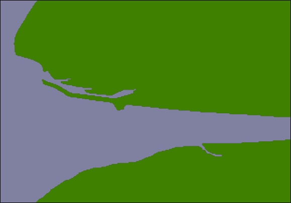
But this section of coastline is actually part of the following GSHHG shoreline feature:
This shoreline polygon is enormous, consisting of over 1.1 million points, and we're only displaying a very small part of it.
Because these shoreline polygons are so big, the map generator needs to read in the entire huge polygon and then discard 99 percent of it to get the desired section of shoreline. Also, because the polygon bounding boxes are so large, many irrelevant polygons are being processed (and then filtered out) to generate the map. This is why showResults.py is so slow.
It is certainly possible to improve the performance of the showResults.py script. As was mentioned in the Best practices section of Chapter 6, Spatial Databases, spatial indexes work best when working with relatively small geometries—and our shoreline polygons are anything but small. However, because the DISTAL application only shows points within a certain distance, we can split these enormous polygons into tiles that are then precalculated and stored in the database.
Let's say that we're going to impose a limit of 100 kilometers to the search radius. We'll also arbitrarily define the tiles to be one whole degree of latitude tall and one whole degree of longitude wide:
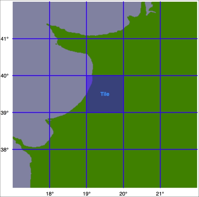
Tip
Note that we could choose any tile size we like but have selected whole degrees of longitude and latitude to make it easy to calculate which tile a given lat/long coordinate is inside. Each tile will be given an integer latitude and longitude value, which we'll call iLat and iLong. We can then calculate the tile to use for any given latitude and longitude like this:
iLat = int(round(latitude))
iLong = int(round(longitude))
We can then simply look up the tile with the given iLat and iLong value.
For each tile, we will calculate the bounds of a rectangle 100 kilometers north, east, west, and south of the tile:
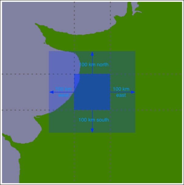
Using the bounding box, we can calculate the intersection of the shoreline data with this bounding box:
Any search done within the tile's boundary, up to a maximum of 100 kilometers in any direction, will only display shorelines within this bounding box. We will store this intersected shoreline into the database along with the lat/long coordinates for the tile, and tell the map generator to use the appropriate tile's outline to display the desired shoreline rather than using the original GSHHG polygons.
Let's write the program that calculates these tiled shorelines. We'll call this program tileShorelines.py. Start by entering the following into this file:
import math

import pyproj
from shapely.geometry import Polygon
from shapely.ops import cascaded_union
import shapely.wkt
import psycopg2

MAX_DISTANCE = 100000 # Maximum search radius, in meters.
We next need a function to calculate the tile bounding boxes. This function, expandRect(), should take a rectangle defined using lat/long coordinates and expand it in each direction by a given number of meters. Using the techniques we have learned, this is straightforward: we can use pyproj to perform an inverse great-circle calculation to calculate four points the given number of meters north, east, south, and west of the original rectangle. This will give us the desired bounding box. Here's what our function will look like:
def expandRect(minLat, minLong, maxLat, maxLong, distance):

    geod = pyproj.Geod(ellps="WGS84")
    midLat  = (minLat + maxLat) / 2.0
    midLong = (minLong + maxLong) / 2.0

    try:
        availDistance = geod.inv(midLong, maxLat, midLong,
                                 +90)[2]
        if availDistance >= distance:
            x,y,angle = geod.fwd(midLong, maxLat, 0, distance)
            maxLat = y
        else:
            maxLat = +90
    except:
        maxLat = +90 # Can't expand north.

    try:
        availDistance = geod.inv(maxLong, midLat, +180,
                                 midLat)[2]
        if availDistance >= distance:
            x,y,angle = geod.fwd(maxLong, midLat, 90,
                                 distance)
            maxLong = x
        else:
            maxLong = +180
    except:
        maxLong = +180 # Can't expand east.

    try:
        availDistance = geod.inv(midLong, minLat, midLong,
                                 -90)[2]
        if availDistance >= distance:
            x,y,angle = geod.fwd(midLong, minLat, 180,
                                 distance)
            minLat = y
        else:
            minLat = -90
    except:
        minLat = -90 # Can't expand south.

    try:
        availDistance = geod.inv(maxLong, midLat, -180,
                                 midLat)[2]
        if availDistance >= distance:
            x,y,angle = geod.fwd(minLong, midLat, 270,
                                 distance)
            minLong = x
        else:
            minLong = -180
    except:
        minLong = -180 # Can't expand west.

return (minLat, minLong, maxLat, maxLong)Using this function, we will be able to calculate the bounding rectangle for a given tile in the following way:
minLat,minLong,maxLat,maxLong = expandRect(iLat, iLong,
                                           iLat+1, iLong+1,
                                           MAX_DISTANCE)
Enter the expandRect() function into your tileShorelines.py script, placing it immediately below the last import statement.
We are now ready to start implementing the tiling algorithm. We'll start by opening a connection to the database:
connection = psycopg2.connect(database="distal",
                              user="distal_user",
                              password="...")
cursor = connection.cursor()We next need to load the shoreline polygons into memory. Here is the necessary code:
shorelines = []

cursor.execute("SELECT ST_AsText(outline) " +
               "FROM shorelines WHERE level=1")

for row in cursor:
    outline = shapely.wkt.loads(row[0])
shorelines.append(outline)Now that we've loaded the shoreline polygons, we can start calculating the contents of each tile. Let's create a list-of-lists that will hold the (possibly clipped) polygons that appear within each tile; add the following to the end of your tileShorelines.py script:
tilePolys = []
for iLat in range(-90, +90):
    tilePolys.append([])
    for iLong in range(-180, +180):
        tilePolys[-1].append([])
For a given iLat/iLong combination, tilePolys[iLat][iLong] will contain a list of the shoreline polygons that appear inside that tile.
We now want to fill the tilePolys array with the portions of the shorelines that will appear within each tile. The obvious way to do this would be to calculate the polygon intersections in the following way:
shorelineInTile = shoreline.intersection(tileBounds)
Unfortunately, this approach would take a very long time to calculate—just as the map generation takes about 2-3 seconds to calculate the visible portion of a shoreline, it takes about 2-3 seconds to perform this intersection on a huge shoreline polygon. Because there are 360 x 180 = 64,800 tiles, it would take several days to complete this calculation using this naive approach.
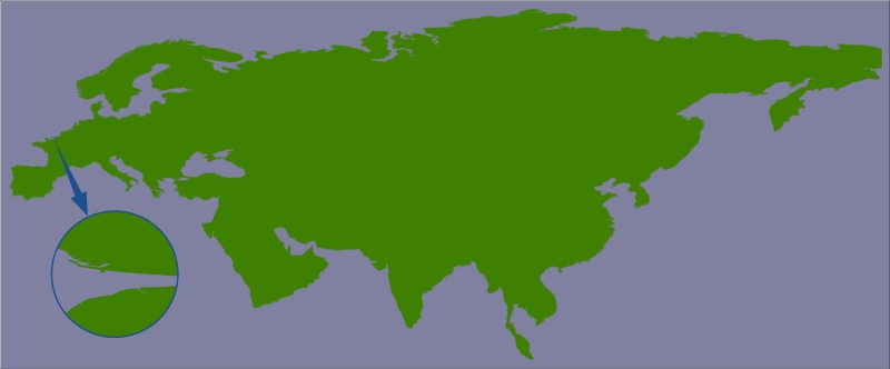
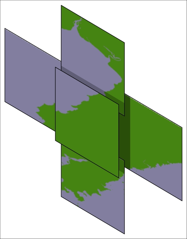
A much faster solution would be to "divide and conquer" the large polygons. We first split the huge shoreline polygon into vertical strips, like this:
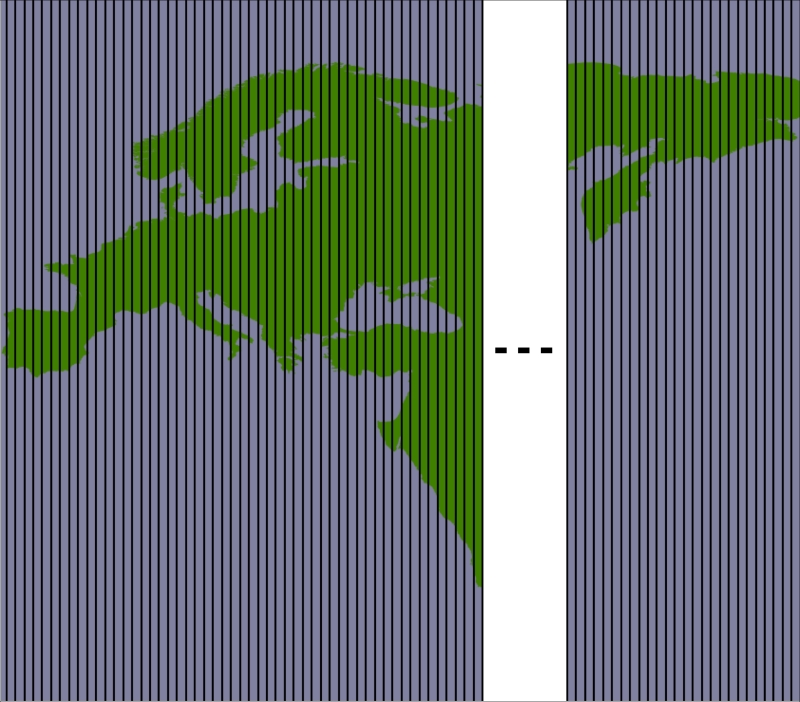
We then split each vertical strip horizontally to give us the individual parts of the polygon, which can be merged into the individual tiles:

By dividing the huge polygons into strips and then further dividing each strip, the intersection process is much faster. Here is the code that performs this intersection; we start by iterating over each shoreline polygon and calculating the polygon's bounds expanded to the nearest whole number:
for shoreline in shorelines:
    minLong,minLat,maxLong,maxLat = shoreline.bounds
    minLong = int(math.floor(minLong))
    minLat  = int(math.floor(minLat))
    maxLong = int(math.ceil(maxLong))
    maxLat  = int(math.ceil(maxLat))
We then split the polygon into vertical strips:
    vStrips = []
    for iLong in range(minLong, maxLong+1):

        stripMinLat  = minLat
        stripMaxLat  = maxLat
        stripMinLong = iLong
        stripMaxLong = iLong + 1

        bMinLat,bMinLong,bMaxLat,bMaxLong = \
                expandRect(stripMinLat, stripMinLong,
                           stripMaxLat, stripMaxLong,
                           MAX_DISTANCE)

        bounds = Polygon([(bMinLong, bMinLat),
                          (bMinLong, bMaxLat),
                          (bMaxLong, bMaxLat),
                          (bMaxLong, bMinLat),
                          (bMinLong, bMinLat)])

        strip = shoreline.intersection(bounds)
        vStrips.append(strip)
Next, we process each vertical strip, splitting the strip into tile-sized blocks and storing the polygons within each block into tilePolys:
    stripNum = 0
    for iLong in range(minLong, maxLong+1):
        vStrip = vStrips[stripNum]
        stripNum = stripNum + 1

        for iLat in range(minLat, maxLat+1):
            bMinLat,bMinLong,bMaxLat,bMaxLong = \
                expandRect(iLat, iLong, iLat+1, iLong+1,
                           MAX_DISTANCE)

            bounds = Polygon([(bMinLong, bMinLat),
                              (bMinLong, bMaxLat),
                              (bMaxLong, bMaxLat),
                              (bMaxLong, bMinLat),
                              (bMinLong, bMinLat)])

            polygon = vStrip.intersection(bounds)
            if not polygon.is_empty:
                tilePolys[iLat][iLong].append(polygon)
We have now stored the tiled polygons into tilePolys for every possible iLat/iLong value.
We're now ready to save the tiled shorelines back into the database. Before we can do that, however, we have to create a new database table to hold the tiled shoreline polygons. Here is the necessary code:
cursor.execute("DROP TABLE IF EXISTS tiled_shorelines")
cursor.execute("CREATE TABLE tiled_shorelines (" +
               "  intLat  INTEGER," +
               "  intLong INTEGER," +
               "  outline GEOMETRY(GEOMETRY, 4326)," +
               "  PRIMARY KEY (intLat, intLong))")
cursor.execute("CREATE INDEX tiledShorelineIndex "+
               "ON tiled_shorelines USING GIST(outline)")
Finally, we can save the tiled shoreline polygons into the tiled_shorelines table:
for iLat in range(-90, +90):
    for iLong in range(-180, +180):
        polygons = tilePolys[iLat][iLong]
        if len(polygons) == 0:
            outline = Polygon()
        else:
            outline = shapely.ops.cascaded_union(polygons)
        wkt = shapely.wkt.dumps(outline)

        cursor.execute("INSERT INTO tiled_shorelines " +
                        "(intLat, intLong, outline) " +
                        "VALUES (%s, %s, " +
                        "ST_GeomFromText(%s))",
                        (iLat, iLong, wkt))
    connection.commit()

connection.close()
This completes our program to tile the shorelines. You can run it by typing the following into a terminal or command-line window:
python tileShorelines.py
Note that it may take several hours for this program to complete because of all the shoreline data that needs to be processed. You may want to leave it running overnight.
Tip
The first time you run the program, you might want to replace this line:
for shoreline in shorelines:
with the following:
for shoreline in shorelines[1:2]:
This will let the program finish in only a minute or two so that you can make sure it's working before removing the [1:2] and running it on the entire shoreline database.
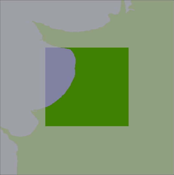
All this gives us a new database table, tiled_shorelines, that holds the shoreline data split into partly overlapping tiles:
Since we can guarantee that all the shoreline data for a given set of search results will be within a single tiled_shoreline record, we can modify our showResults.py script to use the tiled shoreline rather than the raw shoreline data.
To use the tiled shorelines, we are going to make use of a clever feature built into the mapnik.PostGIS data source. The table parameter passed to this data source is normally the name of the database table holding the data to be displayed. However, instead of just supplying a table name, you can pass in an SQL SELECT command to choose the particular subset of records to display. We're going to use this to identify the particular tiled shoreline record to display.
Fortunately, our mapGenerator.generateMap() function accepts a tableName parameter, which is passed directly to the mapnik.PostGIS data source. This allows us to modify the table name passed to the map generator so that the appropriate tiled shoreline record will be used.
To do this, edit the showResults.py script and find the statement that calls the mapGenerator.generateMap() function. This statement currently looks like this:
imgFile = mapGenerator.generateMap("shorelines",
                                   minLong, minLat,
                                   maxLong, maxLat,
                                   MAX_WIDTH, MAX_HEIGHT,
                                   points=points)
Replace this statement with the following:
iLat = int(round(latitude))
iLong = int(round(longitude))

subSelect = "(SELECT outline FROM tiled_shorelines" \
          + " WHERE (intLat={})".format(iLat) \
          + " AND (intLong={})".format(iLong) \
          + ") AS shorelines"

imgFile = mapGenerator.generateMap(subSelect,
                                   minLong, minLat,
                                   maxLong, maxLat,
                                   MAX_WIDTH, MAX_HEIGHT,
                                   points=points)
With these changes, the showResults.py script will use the tiled shorelines rather than the full shoreline data downloaded from GSHHG. Let's now take a look at how much of a performance improvement these tiled shorelines give us.
As soon as you run this new version of the DISTAL application, you should notice an improvement in speed: showResults.py now seems to return its results almost instantly rather than taking a second or more to generate the map. Adding timing code back into the showResults.py script shows how quickly it is running now:
Generating map took 0.1074 seconds
Compare this with how long it took when we were using the full high-resolution shoreline:
Generating map took 3.0208 seconds
As you can see, this is a dramatic improvement in performance: the map generator is now 15-20 times faster than it was, and the total time taken by the showResults.py script is now less than a quarter of a second. That's not bad for a relatively simple change to our underlying map data.