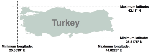
In this slightly contrived example, we will make use of a shapefile to calculate the minimum and maximum latitude/longitude values for each country in the world. This "bounding box" can be used, among other things, to generate a map centered on a particular country. For example, the bounding box for Turkey would look like this:

Start by downloading the World Borders Dataset from http://thematicmapping.org/downloads/world_borders.php. Make sure you download the file named TM_WORLD_BORDERS-0.3.zip rather than the simplified TM_WORLD_BORDERS_SIMPL-0.3.zip file. Decompress the .zip archive and place the various files that make up the shapefile (the .dbf, .prj, .shp, and .shx files) together in a suitable directory.

Next, we need to create a Python program that can read the borders for each country. Fortunately, using OGR to read through the contents of a shapefile is simple:

from osgeo import ogr

shapefile = ogr.Open("TM_WORLD_BORDERS-0.3.shp")
layer = shapefile.GetLayer(0)

for i in range(layer.GetFeatureCount()):
    feature = layer.GetFeature(i)

The feature will consist of a geometry defining the outline of the country, along with a set of attributes providing information about that country. According to the Readme.txt file, the attributes in this shapefile include the ISO-3166 three-letter code for the country (in a field called ISO3) as well as the name for the country (in a field called NAME). This allows us to obtain the country code and name for the feature:

countryCode = feature.GetField("ISO3")
countryName = feature.GetField("NAME")

We can also obtain the country's border polygon using the GetGeometryRef() method:

geometry = feature.GetGeometryRef()

To solve this task, we will need to calculate the bounding box for this geometry. OGR uses the term envelope to refer to the geometry's bounding box, so we can get the bounding box in the following way:

minLong,maxLong,minLat,maxLat = geometry.GetEnvelope()

Let's put all this together into a complete working program:

# calcBoundingBoxes.py

from osgeo import ogr

shapefile = ogr.Open("TM_WORLD_BORDERS-0.3.shp")
layer = shapefile.GetLayer(0)

countries = [] # List of (code, name, minLat, maxLat,
               # minLong, maxLong) tuples.

for i in range(layer.GetFeatureCount()):
    feature = layer.GetFeature(i)
    countryCode = feature.GetField("ISO3")
    countryName = feature.GetField("NAME")
    geometry = feature.GetGeometryRef()
    minLong,maxLong,minLat,maxLat = geometry.GetEnvelope()

    countries.append((countryName, countryCode,
                      minLat, maxLat, minLong, maxLong))

countries.sort()

for name,code,minLat,maxLat,minLong,maxLong in countries:
    print("{} ({}) lat={:.4f}..{:.4f},long={:.4f}..{:.4f}"
        .format(name,code,minLat,maxLat,minLong,maxLong))

Running this program produces the following output:

% python calcBoundingBoxes.py
Afghanistan (AFG) lat=29.4061..38.4721, long=60.5042..74.9157
Albania (ALB) lat=39.6447..42.6619, long=19.2825..21.0542
Algeria (DZA) lat=18.9764..37.0914, long=-8.6672..11.9865
...

In this recipe, we will make use of the World Borders Dataset to obtain polygons defining the borders of Thailand and Myanmar. We will then transfer these polygons into Shapely and use Shapely's capabilities to calculate the common border between these two countries, saving the result into another shapefile.

If you haven't already done so, download the World Borders Dataset from the Thematic Mapping web site, http://thematicmapping.org/downloads/world_borders.php.

The World Borders Dataset conveniently includes the ISO-3166 two-character country code for each feature, so we can identify the features corresponding to Thailand and Myanmar as we read through the shapefile. We can then extract the outline of each country, converting the outlines into Shapely geometry objects. Here is the relevant code, which forms the start of our calcCommonBorders.py program:

# calcCommonBorders.py

import os, os.path, shutil
from osgeo import ogr, osr
import shapely.wkt

shapefile = ogr.Open("TM_WORLD_BORDERS-0.3.shp")
layer = shapefile.GetLayer(0)

thailand = None
myanmar = None

for i in range(layer.GetFeatureCount()):
    feature = layer.GetFeature(i)
    if feature.GetField("ISO2") == "TH":
        geometry = feature.GetGeometryRef()
        thailand = shapely.wkt.loads(geometry.ExportToWkt())
    elif feature.GetField("ISO2") == "MM":
        geometry = feature.GetGeometryRef()
        myanmar = shapely.wkt.loads(geometry.ExportToWkt())

Now that we have the country outlines in Shapely, we can use Shapely's computational geometry capabilities to calculate the common border between these two countries:

commonBorder = thailand.intersection(myanmar)

The result will be a LineString (or a MultiLineString if the border is broken up into more than one part). Let's now save this common border into a new shapefile:

if os.path.exists("common-border"):
    shutil.rmtree("common-border")
os.mkdir("common-border")

spatialReference = osr.SpatialReference()
spatialReference.SetWellKnownGeogCS('WGS84')

driver = ogr.GetDriverByName("ESRI Shapefile")
dstPath = os.path.join("common-border", "border.shp")
dstFile = driver.CreateDataSource(dstPath)
dstLayer = dstFile.CreateLayer("layer", spatialReference)

wkt = shapely.wkt.dumps(commonBorder)

feature = ogr.Feature(dstLayer.GetLayerDefn())
feature.SetGeometry(ogr.CreateGeometryFromWkt(wkt))
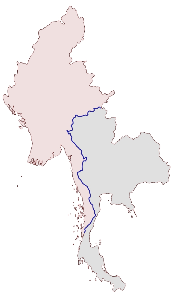
dstLayer.CreateFeature(feature)

If we were to display the results on a map, we could clearly see the common border between these two countries:

The contents of the common-border/border.shp shapefile is represented by the heavy line along the countries' common border.

Note that we will use this shapefile later in this chapter to calculate the length of the Thailand-Myanmar border, so make sure you generate and keep a copy of this shapefile.

A digital elevation map (DEM) is a raster geospatial data format where each pixel value (or cell) represents the height of a point on the earth's surface. We encountered DEM files in the previous chapter, where we saw two examples of data sources that supply this type of information: the National Elevation Dataset covering the United States, and GLOBE which provides DEM files covering the entire Earth.

Because a DEM file contains elevation data, it can be interesting to analyze the elevation values for a given area. For example, we could draw a histogram showing how much of a country's area is at a certain elevation. Let's take some DEM data from the GLOBE dataset and calculate an elevation histogram using that data.

To keep things simple, we will choose a small country surrounded by ocean: New Zealand.

To download the DEM data, go to the GLOBE web site (http://www.ngdc.noaa.gov/mgg/topo/globe.html) and click on the Get Data Online hyperlink. We're going to use the data already calculated for this area of the world, so click on the Any or all 16 "tiles" hyperlink. New Zealand is in tile L, so click on the hyperlink for this tile to download it.

The file you download will be called l10g.zip (or l10g.gz if you chose to download the tile in GZIP format). If you decompress it, you will end up with a single file called l10g, containing the raw elevation data.

By itself, this file isn't very useful—it needs to be georeferenced onto the earth's surface so that you can match up each elevation value with its position on the earth. To do this, you need to download the associated header file. Suitable header files for the premade tiles can be found at http://www.ngdc.noaa.gov/mgg/topo/elev/ esri/hdr. Download the file named l10g.hdr and place it into the same directory as the l10g file you downloaded earlier. You can then read the DEM file using GDAL, just like we did earlier:

from osgeo import gdal
dataset = gdal.Open("l10g")

You probably noticed when you downloaded the l10g tile that it covers much more than just New Zealand—all of Australia is included, as well as Malaysia, Papua New Guinea, and several other east-Asian countries. To work with the elevation data for just New Zealand, we will need to identify the relevant portion of the raster DEM, that is, the range of x and y coordinates that cover New Zealand. We will start by looking at a map and identifying the minimum and maximum latitude/longitude values that enclose all of New Zealand, but no other country:

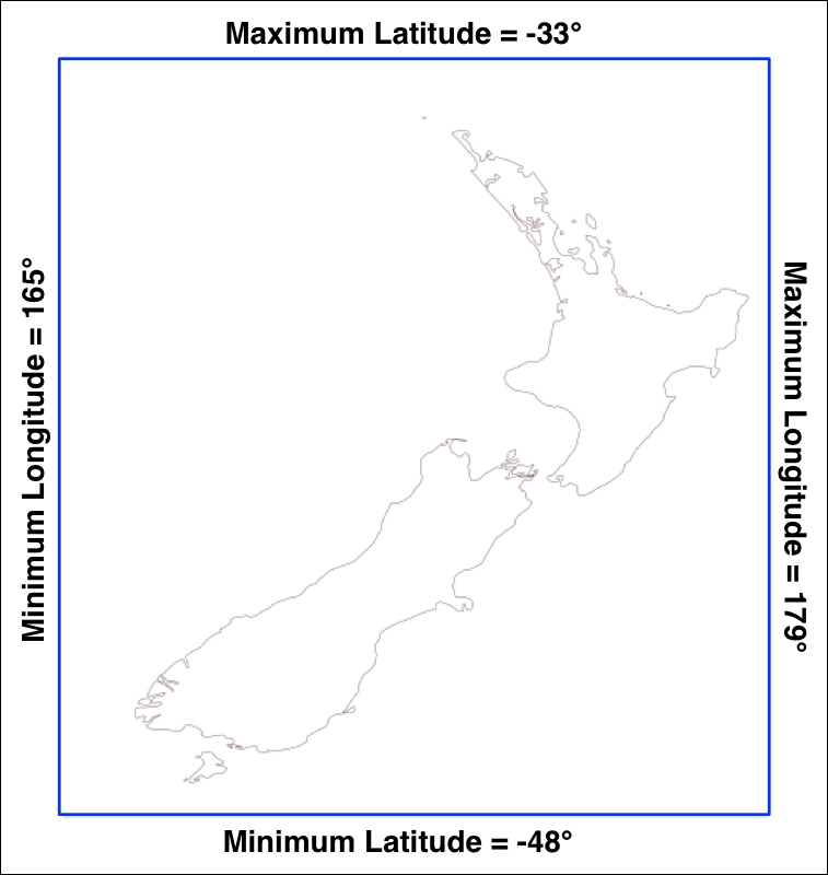
Rounded to the nearest degree, we get a longitude/latitude bounding box of (165, -48)...(179, -33). This is the area we want to scan to cover all of New Zealand.

There is, however, a problem: the raster data consists of pixels or "cells" identified by x and y coordinates, not longitude and latitude values. We have to convert from longitudes and latitudes to x and y coordinates. To do this, we need to make use of GDAL's coordinate transformation features.

We'll start by obtaining our dataset's coordinate transformation:

t = dataset.GetGeoTransform()

Using this transformation, we can convert an (x, y) coordinate to its corresponding latitude and longitude value. In this case, however, we want to do the opposite—we want to take a latitude and longitude and calculate the associated x and y coordinates. To do this, we have to invert the transformation. Once again, GDAL will do this for us:

success,tInverse = gdal.InvGeoTransform(t)
if not success:
    print("Failed!")
    sys.exit(1)

Now that we have the inverse transformation, it is possible to convert from a latitude and longitude to an x and y coordinate, like this:

x,y = gdal.ApplyGeoTransform(tInverse, longitude, latitude)

Using this, we can finally identify the minimum and maximum (x, y) coordinates that cover the area we are interested in:

x1,y1 = gdal.ApplyGeoTransform(tInverse, minLong, minLat)
x2,y2 = gdal.ApplyGeoTransform(tInverse, maxLong, maxLat)

minX = int(min(x1, x2))
maxX = int(max(x1, x2))
minY = int(min(y1, y2))
maxY = int(max(y1, y2))

Now that we know the x and y coordinates for the portion of the DEM that we're interested in, we can use GDAL to read in the individual height values. We start by obtaining the raster band that contains the DEM data:

band = dataset.GetRasterBand(1)

We next want to read the elevation values from our raster band. If you remember, there are two ways you can use GDAL to read raster data: as raw binary data, which you then extract using the struct module, or using the NumPy library to automatically read data into an array.

Let's assume that you don't have NumPy installed; we'll use the struct method instead. Using the technique we covered in Chapter 3, Python Libraries for Geospatial Development, we can use the ReadRaster() method to read the raw binary data and then the struct.unpack() function to convert the binary data to a list of elevation values. Here is the relevant code:

fmt = "<" + ("h" * width)
scanline = band.ReadRaster(X, y, width, height,
                           width, height, gdalconst.GDT_Int16)
values = struct.unpack(fmt, scanline)

Putting all this together, we can use GDAL to open the raster data file and read all the elevation values within the bounding box surrounding New Zealand. We'll then count how often each elevation value occurs and print out a simple histogram using the elevation values. Here is the resulting code:

# histogram.py

import sys, struct
from osgeo import gdal
from osgeo import gdalconst

minLat  = -48
maxLat  = -33
minLong = 165
maxLong = 179

dataset = gdal.Open("l10g")
band = dataset.GetRasterBand(1)

t = dataset.GetGeoTransform()
success,tInverse = gdal.InvGeoTransform(t)
if not success:
    print("Failed!")
    sys.exit(1)

x1,y1 = gdal.ApplyGeoTransform(tInverse, minLong, minLat)
x2,y2 = gdal.ApplyGeoTransform(tInverse, maxLong, maxLat)

minX = int(min(x1, x2))
maxX = int(max(x1, x2))
minY = int(min(y1, y2))
maxY = int(max(y1, y2))

width = (maxX - minX) + 1
fmt = "<" + ("h" * width)

histogram = {} # Maps elevation to number of occurrences.

for y in range(minY, maxY+1):
    scanline = band.ReadRaster(minX, y, width, 1,
                               width, 1,
                               gdalconst.GDT_Int16)
    values = struct.unpack(fmt, scanline)

    for value in values:
        try:
            histogram[value] += 1
        except KeyError:
            histogram[value] = 1

for height in sorted(histogram.keys()):
    print(height, histogram[height])

If you run this, you will see a list of heights (in meters) and how many cells have that height value:

-500 2607581
1 6641
2 909
3 1628
...
3097 1
3119 2
3173 1

This reveals one final problem: there is a large number of cells with an elevation value of -500. What is going on here? Clearly, -500 is not a valid height value. The GLOBE documentation provides the answer:

So all those points with a value of -500 represent cells that are over the ocean. If you remember from our description of the GDAL library in Chapter 3, Python Libraries for Geospatial Development, GDAL includes a no data value for exactly this purpose. Indeed, the gdal.RasterBand object has a GetNoDataValue() method that will tell us what this value is. This allows us to add the following highlighted line to our program to exclude the cells without any data:

for value in values:
    if value != band.GetNoDataValue():
        try:
            histogram[value] += 1
        except KeyError:
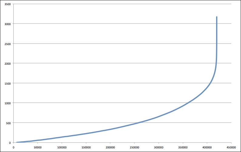
            histogram[value] = 1

This finally gives us a histogram of the heights across New Zealand. You could create a graph using this data if you wished. For example, the following chart shows the total number of pixels at or below a given height: