Table of Contents for
Python Geospatial Development - Third Edition
 Python Geospatial Development - Third Edition
Published by
Packt Publishing, 2016
Python Geospatial Development - Third Edition
Published by
Packt Publishing, 2016
- Cover
- Table of Contents
- Python Geospatial Development Third Edition
- Python Geospatial Development Third Edition
- Credits
- About the Author
- About the Reviewer
- www.PacktPub.com
- Preface
- What you need for this book
- Who this book is for
- Conventions
- Reader feedback
- Customer support
- 1. Geospatial Development Using Python
- Geospatial development
- Applications of geospatial development
- Recent developments
- Summary
- 2. GIS
- GIS data formats
- Working with GIS data manually
- Summary
- 3. Python Libraries for Geospatial Development
- Dealing with projections
- Analyzing and manipulating Geospatial data
- Visualizing geospatial data
- Summary
- 4. Sources of Geospatial Data
- Sources of geospatial data in raster format
- Sources of other types of geospatial data
- Choosing your geospatial data source
- Summary
- 5. Working with Geospatial Data in Python
- Working with geospatial data
- Changing datums and projections
- Performing geospatial calculations
- Converting and standardizing units of geometry and distance
- Exercises
- Summary
- 6. Spatial Databases
- Spatial indexes
- Introducing PostGIS
- Setting up a database
- Using PostGIS
- Recommended best practices
- Summary
- 7. Using Python and Mapnik to Generate Maps
- Creating an example map
- Mapnik concepts
- Summary
- 8. Working with Spatial Data
- Designing and building the database
- Downloading and importing the data
- Implementing the DISTAL application
- Using DISTAL
- Summary
- 9. Improving the DISTAL Application
- Dealing with the scale problem
- Performance
- Summary
- 10. Tools for Web-based Geospatial Development
- A closer look at three specific tools and techniques
- Summary
- 11. Putting It All Together – a Complete Mapping System
- Designing the ShapeEditor
- Prerequisites
- Setting up the database
- Setting up the ShapeEditor project
- Defining the ShapeEditor's applications
- Creating the shared application
- Defining the data models
- Playing with the admin system
- Summary
- 12. ShapeEditor – Importing and Exporting Shapefiles
- Importing shapefiles
- Exporting shapefiles
- Summary
- 13. ShapeEditor – Selecting and Editing Features
- Editing features
- Adding features
- Deleting features
- Deleting shapefiles
- Using the ShapeEditor
- Further improvements and enhancements
- Summary
- Index
In Chapter 2, GIS, we saw that a datum is a mathematical model of the earth's shape, while a projection is a way of translating points on the earth's surface into points on a two-dimensional map. There are a large number of available datums and projections—whenever you are working with geospatial data, you must know which datum and which projection (if any) your data uses. If you are combining data from multiple sources, you will often have to change your geospatial data from one datum to another or from one projection to another.
In this recipe, we will work with two shapefiles that have different projections. We haven't yet encountered any geospatial data that uses a projection—all the data we've seen so far used geographic (unprojected) latitude and longitude values. So, let's start by downloading some geospatial data in the Universal Transverse Mercator (UTM) projection.
The WebGIS web site (http://www.webgis.com) provides shapefiles describing land use and land cover, called LULC data files. For this example, we will download a shapefile for southern Florida (Dade County, to be exact), which uses the UTM projection.
You can download this shapefile from http://www.webgis.com/MAPS/fl/lulcutm/miami.zip.
The decompressed directory contains the shapefile, miami.shp, along with a datum_reference.txt file describing the shapefile's coordinate system. This file tells us the following:
The LULC shape file was generated from the original USGS GIRAS LULC file by Lakes Environmental Software.
Datum: NAD83
Projection: UTM
Zone: 17
Data collection date by U.S.G.S.: 1972
Reference: http://edcwww.cr.usgs.gov/products/landcover/lulc.html
So, this particular shapefile uses UTM zone 17 projection and a datum of NAD83.
Let's take a second shapefile, this time in geographic coordinates. We'll use the GSHHS shoreline database, which uses the WGS84 datum and geographic (latitude/longitude) coordinates.
Tip
You don't need to download the GSHHS database for this example; while we will display a map overlaying the LULC data over the top of the GSHHS data, you only need the LULC shapefile to complete this recipe. Drawing maps such as the one shown in this recipe will be covered in Chapter 7, Using Python and Mapnik to Generate Maps.
We can't directly compare the coordinates in these two shapefiles; the LULC shapefile has coordinates measured in UTM (that is, in meters from a given reference line), while the GSHHS shapefile has coordinates in latitude and longitude values (in decimal degrees):
LULC:  x=485719.47, y=2783420.62
       x=485779.49, y=2783380.63
       x=486129.65, y=2783010.66
       ...

GSHHS: x=180.0000, y=68.9938
       x=180.0000, y=65.0338
       x=179.9984, y=65.0337
Before we can combine these two shapefiles, we first have to convert them to use the same projection. We'll do this by converting the LULC shapefile from UTM-17 to geographic (latitude/longitude) coordinates. Doing this requires us to define an OGR coordinate transformation and then apply that transformation to each of the features in the shapefile.
Here is how you can define a coordinate transformation using OGR:
from osgeo import osr

srcProjection = osr.SpatialReference()
srcProjection.SetUTM(17)

dstProjection = osr.SpatialReference()
dstProjection.SetWellKnownGeogCS('WGS84') # Lat/long.

transform = osr.CoordinateTransformation(srcProjection,
                                         dstProjection)
Using this transformation, we can transform each of the features in the shapefile from UTM projections back into geographic coordinates:
for i in range(layer.GetFeatureCount()):
    feature = layer.GetFeature(i)
    geometry = feature.GetGeometryRef()
    geometry.Transform(transform)
Putting all this together with the techniques we explored earlier for copying the features from one shapefile to another, we end up with the following complete program:
# changeProjection.py

import os, os.path, shutil
from osgeo import ogr
from osgeo import osr
from osgeo import gdal

# Define the source and destination projections, and a
# transformation object to convert from one to the other.

srcProjection = osr.SpatialReference()
srcProjection.SetUTM(17)

dstProjection = osr.SpatialReference()
dstProjection.SetWellKnownGeogCS('WGS84') # Lat/long.

transform = osr.CoordinateTransformation(srcProjection,
                                         dstProjection)

# Open the source shapefile.

srcFile = ogr.Open("miami/miami.shp")
srcLayer = srcFile.GetLayer(0)

# Create the dest shapefile, and give it the new projection.

if os.path.exists("miami-reprojected"):
    shutil.rmtree("miami-reprojected")
os.mkdir("miami-reprojected")

driver = ogr.GetDriverByName("ESRI Shapefile")
dstPath = os.path.join("miami-reprojected", "miami.shp")
dstFile = driver.CreateDataSource(dstPath)
dstLayer = dstFile.CreateLayer("layer", dstProjection)

# Reproject each feature in turn.

for i in range(srcLayer.GetFeatureCount()):
    feature = srcLayer.GetFeature(i)
    geometry = feature.GetGeometryRef()

    newGeometry = geometry.Clone()
    newGeometry.Transform(transform)

    feature = ogr.Feature(dstLayer.GetLayerDefn())
    feature.SetGeometry(newGeometry)
    dstLayer.CreateFeature(feature)
Note
Note that this example doesn't copy field values into the new shapefile; if your shapefile has metadata, you will want to copy the fields across as you create each new feature. Also, the preceding code assumes that the miami.shp shapefile has been placed into a miami subdirectory; you'll need to change the ogr.Open() statement to use the appropriate path name if you've stored this shapefile in a different place.
After running this program over the miami.shp shapefile, the coordinates for all the features in the shapefile will have been converted from UTM-17 to geographic coordinates:
Before reprojection:  x=485719.47, y=2783420.62
                      x=485779.49, y=2783380.63
                      x=486129.65, y=2783010.66
                      ...

  After reprojection: x=-81.1417, y=25.1668
                      x=-81.1411, y=25.1664
                      x=-81.1376, y=25.1631
To see whether this worked, let's draw a map showing the reprojected LULC data overlaid on top of the GSHHS shoreline data:
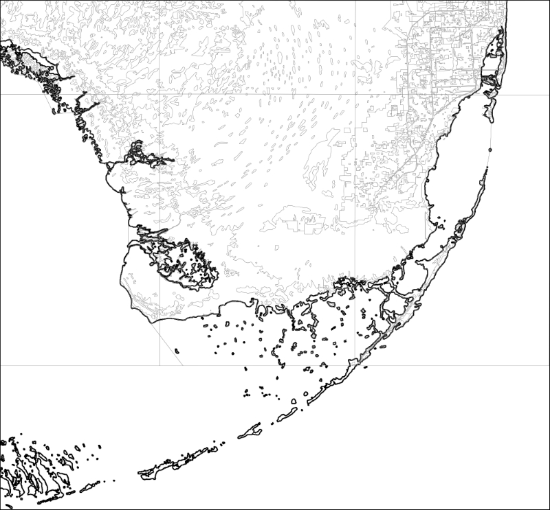
The light gray outlines show the various polygons within the LULC shapefile, while the black outline shows the shoreline as defined by the GLOBE shapefile. Both of these shapefiles now use geographic coordinates and, as you can see, the coastlines match exactly.
For this example, we will need to obtain some geospatial data that uses the NAD27 datum. This datum dates back to 1927 and was commonly used for North American geospatial analysis up until the 1980s, when it was replaced by NAD83.
The US Geological Survey makes available a set of road data that uses the older NAD27 datum. To obtain this data, go to http://pubs.usgs.gov/dds/dds-81/TopographicData/Roads and download the files named roads.dbf, roads.prj, roads.shp, and roads.shx. These four files together make up the "roads" shapefile. Place them into a directory named roads.
This sample shapefile covers an area of the Sierra Nevada mountains in the United States, including a portion of both California and Nevada. The town of Bridgeport, CA, is covered by this shapefile.
Using the ogrinfo command-line tool, we can see that this shapefile does indeed use the older NAD27 datum:
% ogrinfo -so roads.shp roads
INFO: Open of `roads.shp'
      using driver `ESRI Shapefile' successful.

Layer name: roads
Geometry: Line String
Feature Count: 10050
Extent: (-119.637220, 37.462695) - (-117.834877, 38.705226)
Layer SRS WKT:
GEOGCS["GCS_North_American_1927",
    DATUM["North_American_Datum_1927",
        SPHEROID["Clarke_1866",6378206.4,294.9786982]],
    PRIMEM["Greenwich",0],
    UNIT["Degree",0.0174532925199433]]
...
If we were to assume that this shapefile uses the more common WGS84 datum, all the features would appear in the wrong places:
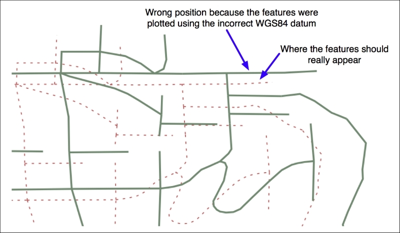
To make the features appear in the correct places and to be able to combine these features with other data that uses the WGS84 datum, we need to convert the shapefile to use WGS84. Changing a shapefile from one datum to another requires the same basic process we used earlier to change a shapefile from one projection to another.
First, you choose the source and destination datums and define a coordinate transformation to convert from one to the other:
srcDatum = osr.SpatialReference()
srcDatum.SetWellKnownGeogCS('NAD27')

dstDatum = osr.SpatialReference()
dstDatum.SetWellKnownGeogCS('WGS84')

transform = osr.CoordinateTransformation(srcDatum, dstDatum)
You then process each feature in the shapefile, transforming the feature's geometry using the coordinate transformation:
for i in range(srcLayer.GetFeatureCount()):
    feature = srcLayer.GetFeature(i)
    geometry = feature.GetGeometryRef()
    geometry.Transform(transform)
Here is the complete Python program to convert the roads shapefile from the NAD27 datum to WGS84:
# changeDatum.py

import os, os.path, shutil
from osgeo import ogr
from osgeo import osr
from osgeo import gdal

# Define the source and destination datums, and a
# transformation object to convert from one to the other.

srcDatum = osr.SpatialReference()
srcDatum.SetWellKnownGeogCS('NAD27')

dstDatum = osr.SpatialReference()
dstDatum.SetWellKnownGeogCS('WGS84')

transform = osr.CoordinateTransformation(srcDatum, dstDatum)

# Open the source shapefile.

srcFile = ogr.Open("roads/roads.shp")
srcLayer = srcFile.GetLayer(0)

# Create the dest shapefile, and give it the new projection.

if os.path.exists("roads-reprojected"):
    shutil.rmtree("roads-reprojected")
os.mkdir("roads-reprojected")

driver = ogr.GetDriverByName("ESRI Shapefile")
dstPath = os.path.join("roads-reprojected", "roads.shp")
dstFile = driver.CreateDataSource(dstPath)
dstLayer = dstFile.CreateLayer("layer", dstDatum)

# Reproject each feature in turn.

for i in range(srcLayer.GetFeatureCount()):
    feature = srcLayer.GetFeature(i)
    geometry = feature.GetGeometryRef()

    newGeometry = geometry.Clone()
    newGeometry.Transform(transform)

    feature = ogr.Feature(dstLayer.GetLayerDefn())
    feature.SetGeometry(newGeometry)
    dstLayer.CreateFeature(feature)
The preceding code assumes that the roads folder is in the same directory as the Python script itself; if you placed this folder somewhere else, you'll need to change the ogr.Open() statement to use the appropriate directory path.
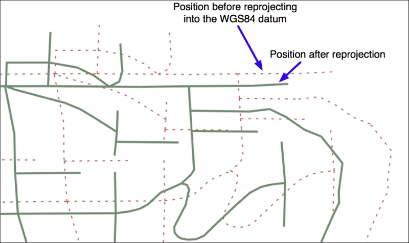
If we now plot the reprojected features using the WGS84 datum, the features will appear in the correct places: