Table of Contents for
Python Geospatial Development - Third Edition
 Python Geospatial Development - Third Edition
Published by
Packt Publishing, 2016
Python Geospatial Development - Third Edition
Published by
Packt Publishing, 2016
- Cover
- Table of Contents
- Python Geospatial Development Third Edition
- Python Geospatial Development Third Edition
- Credits
- About the Author
- About the Reviewer
- www.PacktPub.com
- Preface
- What you need for this book
- Who this book is for
- Conventions
- Reader feedback
- Customer support
- 1. Geospatial Development Using Python
- Geospatial development
- Applications of geospatial development
- Recent developments
- Summary
- 2. GIS
- GIS data formats
- Working with GIS data manually
- Summary
- 3. Python Libraries for Geospatial Development
- Dealing with projections
- Analyzing and manipulating Geospatial data
- Visualizing geospatial data
- Summary
- 4. Sources of Geospatial Data
- Sources of geospatial data in raster format
- Sources of other types of geospatial data
- Choosing your geospatial data source
- Summary
- 5. Working with Geospatial Data in Python
- Working with geospatial data
- Changing datums and projections
- Performing geospatial calculations
- Converting and standardizing units of geometry and distance
- Exercises
- Summary
- 6. Spatial Databases
- Spatial indexes
- Introducing PostGIS
- Setting up a database
- Using PostGIS
- Recommended best practices
- Summary
- 7. Using Python and Mapnik to Generate Maps
- Creating an example map
- Mapnik concepts
- Summary
- 8. Working with Spatial Data
- Designing and building the database
- Downloading and importing the data
- Implementing the DISTAL application
- Using DISTAL
- Summary
- 9. Improving the DISTAL Application
- Dealing with the scale problem
- Performance
- Summary
- 10. Tools for Web-based Geospatial Development
- A closer look at three specific tools and techniques
- Summary
- 11. Putting It All Together – a Complete Mapping System
- Designing the ShapeEditor
- Prerequisites
- Setting up the database
- Setting up the ShapeEditor project
- Defining the ShapeEditor's applications
- Creating the shared application
- Defining the data models
- Playing with the admin system
- Summary
- 12. ShapeEditor – Importing and Exporting Shapefiles
- Importing shapefiles
- Exporting shapefiles
- Summary
- 13. ShapeEditor – Selecting and Editing Features
- Editing features
- Adding features
- Deleting features
- Deleting shapefiles
- Using the ShapeEditor
- Further improvements and enhancements
- Summary
- Index
One of the most enthralling aspects of programs such as Google Earth is the ability to "see" the Earth as you appear to fly above it. This is achieved by displaying satellite and aerial photographs carefully stitched together to provide the illusion that you are viewing the Earth's surface from above.
While writing your own version of Google Earth would be an almost impossible task, it is possible to obtain free satellite imagery in the form of raster-format geospatial data, which you can then use in your own geospatial applications.
Raster data is not just limited to images of the Earth's surface, however; other useful information can be found in raster format—for example, digital elevation maps (DEMs) contain the height of each point on the Earth's surface, which can then be used to calculate the elevation of any desired point. DEM data can also be used to generate two-dimensional images that represent different heights using different shades or colors or to simulate the shading effect of hills using a technique called shaded relief imagery.
In this section, we will look at the world's most comprehensive source of satellite imagery, Landsat, as well as the raster-format data available on the Natural Earth site and some freely-available sources of digital elevation data.
Landsat is an ongoing effort to collect images of the Earth's surface. The name is derived from land and satellite. A group of dedicated satellites have been continuously gathering images since 1972. Landsat imagery includes black and white and traditional red/green/blue (RGB) color images as well as infrared and thermal imaging. The color images are typically at a resolution of 30 meters per pixel, while the black and white images from Landsat 7 are at a resolution of 15 meters per pixel.
The following image shows color-corrected Landsat satellite imagery for the city of Rotorua, New Zealand. The city itself is on the southern (bottom) edge of a lake:
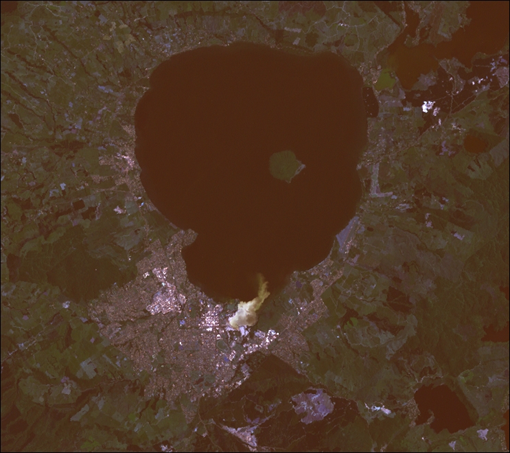
Landsat images are typically available in the form of GeoTIFF files. GeoTIFF is a geospatially tagged TIFF image file format, allowing images to be georeferenced onto the Earth's surface. Most GIS software and tools, including GDAL, are able to read GeoTIFF-formatted files.
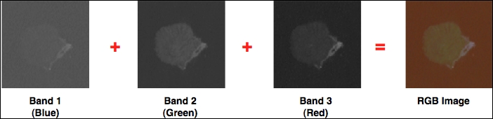
Because the images come directly from a satellite, the files you can download typically store separate bands of data in separate files. Depending on the satellite the data came from, there can be up to eight different bands of data—for example, Landsat 7 generates separate red, green, and blue bands as well as three different infrared bands, a thermal band, and a high-resolution "panchromatic" (black-and-white) band.
To understand how this works, let's take a closer look at the process required to create the preceding image. The raw satellite data consists of eight separate GeoTIFF files, one for each band. band 1 contains the blue color data, band 2 contains the green color data, and band 3 contains the red color data. These separate files can then be combined using GDAL to produce a single color image, as follows:
Another complication with the Landsat data is that the images produced by the satellites are distorted by various factors, including the ellipsoid shape of the Earth, the elevation of the terrain being photographed, and the orientation of the satellite as the image is taken. The raw data is therefore not a completely accurate representation of the features being photographed. Fortunately, a process known as orthorectification can be used to correct these distortions. In most cases, orthorectified versions of the satellite images can be downloaded directly.
The easiest way to access Landsat imagery is to make use of the University of Maryland's Global Land Cover Faci lity web site (http://glcf.umd.edu/data/landsat). Click on the Download via Search and Preview Tool (ESDI) link, and then click on Map Search. Select ETM+ from the Landsat Imagery list, and if you zoom in on the desired part of the Earth, you will see the areas covered by various Landsat images:
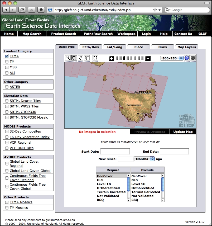
If you choose the selection tool ( ), you will be able to click on a desired area and then select Preview & Download to choose the image to download.
Alternatively, if you know the path and row number of the desired area of the Earth, you can directly access the files via FTP. The path and row number (as well as the world reference system (WRS) number used by the data) can be found on the Preview & Download page:
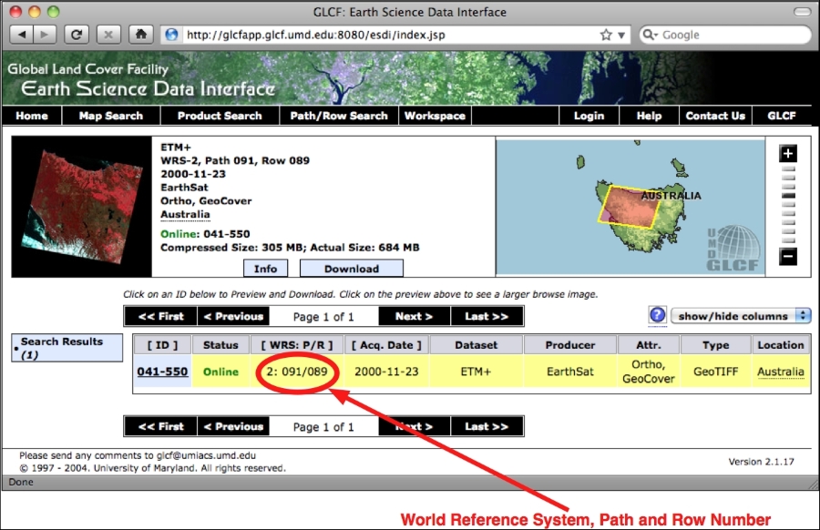
If you want to download the image files via FTP, the main FTP site is at ftp://ftp.glcf.umd.edu/glcf/Landsat.
The directories and files have complex names that include the WRS, the path and row number, the satellite number, the date at which the image was taken, and the band number. For example, a file named p091r089_7t20001123_z55_nn10.tif.gz refers to path 091 and row 089, which happens to be the portion of Tasmania highlighted in the preceding screen snapshot. The 7 refers to the number of the Landsat satellite that took the image, and 20001123 is a datestamp indicating when the image was taken. The final part of the filename, nn10, tells us that the file is for band 1.
By interpreting the filename in this way, you can download the correct files and match the files against the desired bands. For more information on what all these different satellites and bands mean, refer to the documentation links in the Landsat Imagery section in the upper right-hand corner of the Global Land Cover Facility web site (http://glcf.umd.edu/data/landsat).
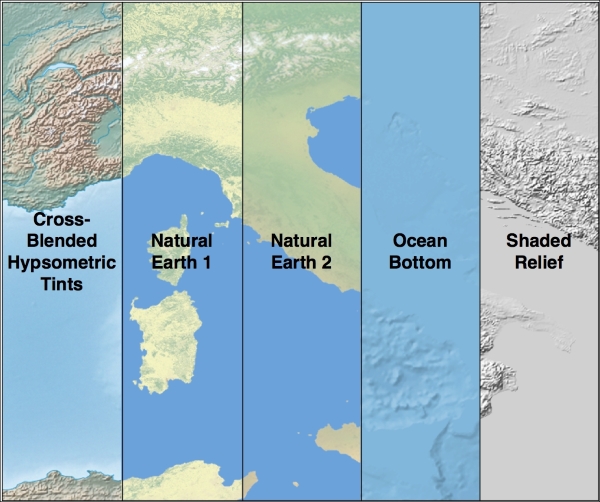
In addition to providing vector map data, the Natural Earth web site (http://www.naturalearthdata.com) makes available five different types of raster maps at both a 1:10-million and 1:50-million scale:
- The rather esoterically-named Cross-Blended Hypsometric Tints provide visualizations where the color is selected based on both elevation and climate. These images are then often combined with shaded-relief images to produce a realistic-looking view of the Earth's surface.
- Natural Earth 1 and Natural Earth 2 are more idealized views of the Earth's surface; they use a light palette and softly blended colors, providing an excellent backdrop for drawing your own geospatial data.
- The Ocean Bottom dataset uses a combination of shaded relief imagery and depth-based coloring to provide a visualization of the ocean floor.
- The Shaded Relief imagery uses greyscale to "shade" the surface of the Earth based on high-resolution elevation data.
The following diagram shows what these raster maps look like:
An additional raster dataset is available that provides bathymetry (underwater depth) visualizations at a 1:50-million scale. The following diagram is an example of the bathymetry data for the oceans surrounding New Zealand:
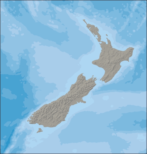
Most of the raster-format data on the Natural Earth site is in the standard TIFF image format. The one exception is the bathymetry data, which is provided in the form of a layered Adobe Photoshop file with differing shades of blue associated with each depth band.
In all cases, the raster data is in geographic (latitude/longitude) projection and uses the standard WGS84 datum, making it easy to translate between latitude and longitude coordinates and pixel coordinates within the raster image.
As with the vector data, the raster-format data on the Natural Earth site is easy to download: simply go to the web site (http://www.naturalearthdata.com) and follow the Get the Data link to download the raster-format data. You can choose to download the data at either a 1:10-million scale or a 1:50-million scale, and you can also choose to download the large- or small-size version of each file.
Once you have downloaded the TIFF format data, you can open the file in an image editor or use a command-line utility such as gdal_translate to manipulate the image. For the bathymetry data, you can open the file directly in Adobe Photoshop or use a cheaper alternative such as GIMP or Flying Meat's Acorn. Each depth band is a separate layer in the file and is associated with a specific shade of blue by default. You can choose different colors if you prefer and select which layers to show or hide. When you are finished, you can flatten the image and save it as a TIFF file for use in your programs.
GLOBE is an international effort to produce high-quality, medium-resolution digital elevation model (DEM) data for the entire world. The result is a set of freely-available DEM files, which can be used for many types of geospatial analysis and development.
The following diagram shows GLOBE DEM data for northern Chile, converted to a grayscale image:
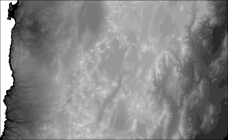
Like all DEM data, GLOBE uses raster values to represent the elevation at a given point on the Earth's surface. In the case of GLOBE, this data consists of 32-bit signed integers representing the height above (or below) sea level, in meters. Each cell or "pixel" within the raster data represents the elevation of a square on the Earth's surface that is 30 arc-seconds of longitude wide and 30 arc-seconds of latitude high:
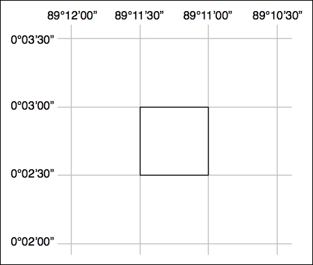
Note that 30 arc-seconds equal approximately 0.00833 degrees of latitude or longitude, which equates to a square roughly one kilometer wide and high. This means that the GLOBE data has a resolution of approximately 1 kilometer per cell or "pixel".
The raw GLOBE data is simply a long list of 32-bit integers in big-endian format, where the cells are read left to right and then top to bottom, like this:
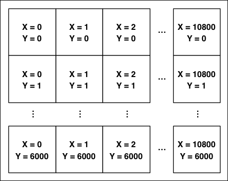
A separate header (.hdr) file provides more detailed information about the DEM data, including the width and height and its georeferenced location. Tools such as GDAL are able to read the raw data as long as the header file is provided.
The main web site for the GLOBE project can be found at http://www.ngdc.noaa.gov/mgg/topo/globe.html, and you can download a detailed manual describing the GLOBE dataset at http://www.ngdc.noaa.gov/mgg/topo/report/globedocumentationmanual.pdf.
The GLOBE elevation data is made available as a series of 16 "tiles" covering the entire Earth's surface. You can download any of the tiles that you wish by clicking on the Get Data Online link from the main page.
Unfortunately, the tile data you download only includes the raw elevation data itself. There is no information provided for georeferencing the elevation data onto the surface of the Earth or to tell GDAL what format the data is in. If you don't want to calculate this information yourself, you will need to download a .hdr file corresponding to each tile. These .hdr files can be found at http://www.ngdc.noaa.gov/mgg/topo/elev/esri/hdr.
Once you have downloaded the data, simply place the raw DEM file into the same directory as the .hdr file. You can then open the file directly using GDAL, like this:
import osgeo.gdal
dataset = osgeo.gdal.Open("j10g.bil")
The dataset will consist of a single band of raster data, which you can then read using GDAL.
Note
To see an example of using GDAL to process DEM data, please refer to the GDAL section in Chapter 3, Python Libraries for Geospatial Development.
The National Elevation Dataset (NED) is a high-resolution digital elevation model provided by the US Geological Survey. It covers the continental United States, Alaska, Hawaii, and other US territories. Most of the United States is covered by elevation data at a resolution of either 30 or 10 meters per cell, with selected areas available at 3 meters per cell. Alaska is generally only available at a resolution of 60 meters per cell.
The following shaded relief image was generated using NED elevation data for the Marin Headlands in San Francisco:
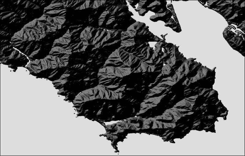
NED data can be downloaded in various formats, including IMG, GeoTIFF, and ArcGRID, all of which can be processed using GDAL.
As with other DEM data, each cell in the raster image represents the height of a given area on the Earth's surface. For NED data, the height is in meters above or below a reference height known as the North American Vertical Datum of 1988. This roughly equates to the height above sea level, allowing for tidal and other variations.
The main web site for the National Elevation Dataset can be found at: http://ned.usgs.gov.
This site describes the NED dataset; to download the data, you'll have to use the National Map Viewer, which is available at http://viewer.nationalmap.gov/viewer/.
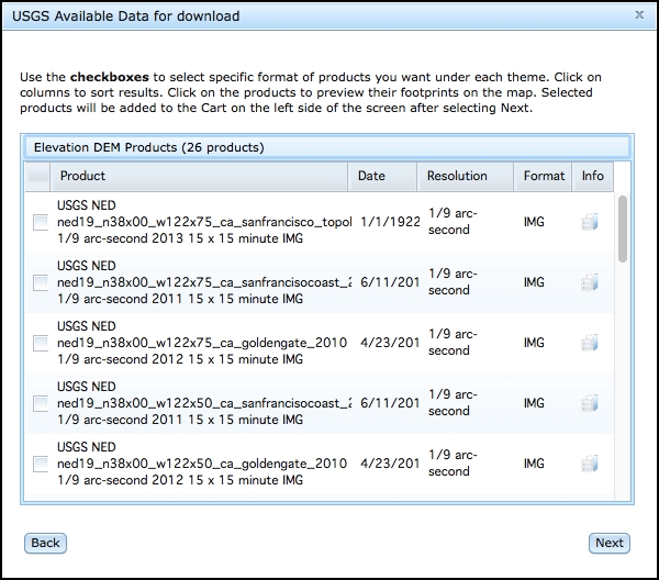
To use the viewer, zoom in to the area you are interested in, and then click on the Download Data link at the top of the page:
Click on the option to download by the current map extent, and then select the Elevation DEM Products option from the provided list. When you click on the Next button, you will be presented with a list of the available DEM datasets that cover the visible portion of the map:
Choose the dataset you are interested in and click on the Info icon beside the dataset.
When you click on the Info icon, a new tab will be opened in your browser, giving you lots of information about the selected dataset. In particular, you will see a map showing the area covered by this dataset:
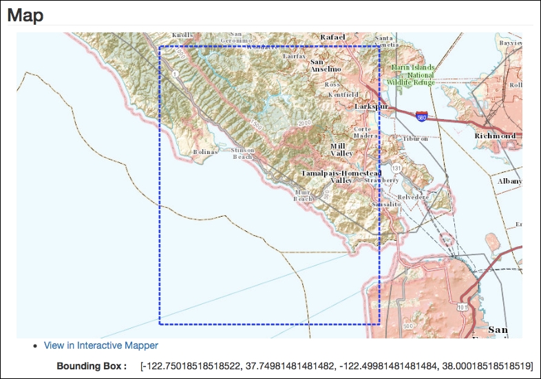
If you scroll down to the Links (External Sources) section of the page, you will see a direct download link for the dataset. Clicking on this will immediately download the file.
You will end up with a compressed .zip format file containing the data you want, along with a large number of metadata files and documentation about the dataset. Once you have decompressed the .zip archive, you can open the dataset in GDAL just like you would open any other raster dataset:
import osgeo.gdal
dataset = osgeo.gdal.Open("dem.tif")
Finally, if you are working with DEM data, you might like to check out the gdaldem utility, which is included as a part of the GDAL download. This program makes it easy to view and manipulate DEM raster data. The preceding shaded relief image was created using this utility, like this:
gdaldem hillshade dem.tif image.tiff