Table of Contents for
Python Geospatial Development - Third Edition
 Python Geospatial Development - Third Edition
Published by
Packt Publishing, 2016
Python Geospatial Development - Third Edition
Published by
Packt Publishing, 2016
- Cover
- Table of Contents
- Python Geospatial Development Third Edition
- Python Geospatial Development Third Edition
- Credits
- About the Author
- About the Reviewer
- www.PacktPub.com
- Preface
- What you need for this book
- Who this book is for
- Conventions
- Reader feedback
- Customer support
- 1. Geospatial Development Using Python
- Geospatial development
- Applications of geospatial development
- Recent developments
- Summary
- 2. GIS
- GIS data formats
- Working with GIS data manually
- Summary
- 3. Python Libraries for Geospatial Development
- Dealing with projections
- Analyzing and manipulating Geospatial data
- Visualizing geospatial data
- Summary
- 4. Sources of Geospatial Data
- Sources of geospatial data in raster format
- Sources of other types of geospatial data
- Choosing your geospatial data source
- Summary
- 5. Working with Geospatial Data in Python
- Working with geospatial data
- Changing datums and projections
- Performing geospatial calculations
- Converting and standardizing units of geometry and distance
- Exercises
- Summary
- 6. Spatial Databases
- Spatial indexes
- Introducing PostGIS
- Setting up a database
- Using PostGIS
- Recommended best practices
- Summary
- 7. Using Python and Mapnik to Generate Maps
- Creating an example map
- Mapnik concepts
- Summary
- 8. Working with Spatial Data
- Designing and building the database
- Downloading and importing the data
- Implementing the DISTAL application
- Using DISTAL
- Summary
- 9. Improving the DISTAL Application
- Dealing with the scale problem
- Performance
- Summary
- 10. Tools for Web-based Geospatial Development
- A closer look at three specific tools and techniques
- Summary
- 11. Putting It All Together – a Complete Mapping System
- Designing the ShapeEditor
- Prerequisites
- Setting up the database
- Setting up the ShapeEditor project
- Defining the ShapeEditor's applications
- Creating the shared application
- Defining the data models
- Playing with the admin system
- Summary
- 12. ShapeEditor – Importing and Exporting Shapefiles
- Importing shapefiles
- Exporting shapefiles
- Summary
- 13. ShapeEditor – Selecting and Editing Features
- Editing features
- Adding features
- Deleting features
- Deleting shapefiles
- Using the ShapeEditor
- Further improvements and enhancements
- Summary
- Index
Shapely is a very capable library for performing various calculations on geospatial data. Let's put it through its paces with a complex, real-world problem.
The US Census Bureau makes available a shapefile containing something called Core Based Statistical Areas (CBSAs), which are polygons defining urban areas with a population of 10,000 or more. At the same time, the GNIS web site provides lists of place names and other details. Using these two data sources, we will identify any parks within or close to an urban area.
Because of the volume of data we are dealing with, we will limit our search to California. It would take a very long time to check all the CBSA polygon/place name combinations for the entire United States; it's possible to optimize the program to do this quickly, but this would make the example too complex for our current purposes.
Let's start by downloading the necessary data. We'll start by downloading a shapefile containing all the core-based statistical areas in the USA. Go to the TIGER web site:
http://census.gov/geo/www/tiger
Click on the TIGER/Line Shapefiles link, then follow the Download option for the latest version of the TIGER/Line shapefiles (as of this writing, it is the 2015 version). Select the FTP Interface option, and your computer will open an FTP session to the appropriate directory. Sign in as a guest, switch to the CBSA directory, and download the appropriate file you find there.
The file you want to download will have a name like tl_XXXX_us_cbsa.zip, where XXXX is the year the data file was created. Once the file has been downloaded, decompress it and place the resulting shapefile into a convenient location so that you can work with it.
You now need to download the GNIS place name data. Go to the GNIS web site, http://geonames.usgs.gov/domestic, and click on the Download Domestic Names hyperlink. Because we only need the data for California, choose this state from the Select state for download popup menu beneath the States, Territories, Associated Areas of the United States section of this page. This will download a file with a name like CA_Features_XXX.txt, where XXX is the date when the file was created. Place this file somewhere convenient, alongside the CBSA shapefile you downloaded earlier.
We're now ready to start writing our code. Let's start by reading through the CBSA urban area shapefile and extracting the polygons that define the outline of each urban area, as a Shapely geometry object:
shapefile = ogr.Open("tl_2015_us_cbsa.shp")
layer = shapefile.GetLayer(0)

for i in range(layer.GetFeatureCount()):
    feature = layer.GetFeature(i)
    geometry = feature.GetGeometryRef()
    wkt = geometry.ExportToWkt()
    outline = shapely.wkt.loads(wkt)
Next, we need to scan through the CA_Features_XXX.txt file to identify the features marked as parks. For each of these features, we want to extract the name of the feature and its associated latitude and longitude. Here's how we might do this:
f = open("CA_Features_XXX.txt", "r")
for line in f.readlines():
    chunks = line.rstrip().split("|")
    if chunks[2] == "Park":
        name = chunks[1]
        latitude = float(chunks[9])
        longitude = float(chunks[10])
Remember that the GNIS place name database is a "pipe-delimited" text file. That's why we have to split the line up using line.rstrip().split("|").
Now comes the fun part: we need to figure out which parks are within or close to each urban area. There are two ways we could do this, either of which will work:
- We could use the
outline.distance()method to calculate the distance between the outline and aPointobject representing the park's location: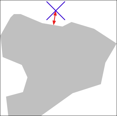
- We could dilate the polygon using the
outline.buffer()method, and then see whether the resulting polygon contained the desired point: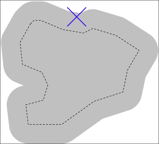
The second option is faster when dealing with a large number of points, as we can pre-calculate the dilated polygons and then use them to compare against each point in turn. Let's take this option:
# findNearbyParks.py

from osgeo import ogr
import shapely.geometry
import shapely.wkt

MAX_DISTANCE = 0.1 # Angular distance; approx 10 km.

print("Loading urban areas...")

urbanAreas = {} # Maps area name to Shapely polygon.

shapefile = ogr.Open("tl_2015_us_cbsa.shp")
layer = shapefile.GetLayer(0)

for i in range(layer.GetFeatureCount()):
    print("Dilating feature {} of {}"
          .format(i, layer.GetFeatureCount()))
    feature = layer.GetFeature(i)
    name = feature.GetField("NAME")
    geometry = feature.GetGeometryRef()
    outline = shapely.wkt.loads(geometry.ExportToWkt())
    dilatedOutline = outline.buffer(MAX_DISTANCE)
    urbanAreas[name] = dilatedOutline

print("Checking parks...")

f = open("CA_Features_XXX.txt", "r")
for line in f.readlines():
    chunks = line.rstrip().split("|")
    if chunks[2] == "Park":
        parkName = chunks[1]
        latitude = float(chunks[9])
        longitude = float(chunks[10])

        pt = shapely.geometry.Point(longitude, latitude)

        for urbanName,urbanArea in urbanAreas.items():
            if urbanArea.contains(pt):
                print("{} is in or near {}"
                      .format(parkName, urbanName))
f.close()It will take a few minutes to run this program, after which you will get a complete list of all the parks that are in or close to an urban area:
% python findNearbyParks.py
Loading urban areas...
Checking parks...
Imperial National Wildlife Refuge is in or near El Centro, CA
Imperial National Wildlife Refuge is in or near Yuma, AZ
Cibola National Wildlife Refuge is in or near El Centro, CA
Twin Lakes State Beach is in or near Santa Cruz-Watsonville, CA
Admiral William Standley State Recreation Area is in or near Ukiah, CA
...
Note that our program uses angular distances to decide whether a park is in or near a given urban area. As we mentioned in Chapter 2, GIS, an angular distance is the angle between two lines going out from the center of the earth to its surface:
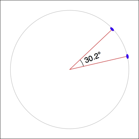
Because we are dealing with data for California, where one degree of angular measurement roughly equals 100 kilometers on the earth's surface, an angular measurement of 0.1 roughly equals a real-world distance of 10 km.
Using angular measurements makes the distance calculation easy and quick to calculate, though it doesn't give an exact distance on the earth's surface. If your application requires exact distances, you could start by using an angular distance to filter out the features obviously too far away and then obtain an exact result for the remaining features by calculating the point on the polygon's boundary that is closest to the desired point and calculating the linear distance between the two points. You would then discard the points that exceed your desired exact linear distance. Implementing this would be an interesting challenge, though not one we will examine in this book.