Recommended best practices

In this section, we will look at a number of practical things you can do to ensure that your geospatial databases work as efficiently and effectively as possible.

Best practice: use the database to keep track of spatial references

As we've seen in earlier chapters, different sets of geospatial data use different coordinate systems, datums, and projections. Consider, for example, the following two geometry objects:

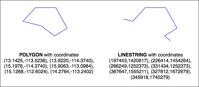
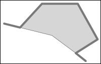
The geometries are represented as a series of coordinates, which are nothing more than numbers. By themselves, these numbers aren't particularly useful—you need to position these coordinates onto the earth's surface by identifying the spatial reference (coordinate system, datum, and projection) used by the geometry. In this case, the Polygon is using unprojected lat/long coordinates in the WGS84 datum, while the LineString is using coordinates defined in meters using the UTM zone 12N projection. Once you know the spatial reference, you can place the two geometries onto the earth's surface. This reveals that the two geometries actually overlap, even though the numbers they use are completely different:

In all but the simplest databases, it is recommended that you store the spatial reference for each feature directly in the database itself. This makes it easy to keep track of which spatial reference is used by each feature. It also allows the queries and database commands you write to be aware of the spatial reference and enables you to transform geometries from one spatial reference to another as necessary in your spatial queries.

Spatial references are generally referred to using a simple integer value called a spatial reference identifier (SRID). While you could choose arbitrary SRID values to represent various spatial references, it is strongly recommended that you use the European Petroleum Survey Group (EPSG) numbers as standard SRID values. Using this internationally recognized standard makes your data interchangeable with other databases and allows tools such as OGR and Mapnik to identify the spatial reference used by your data.

To learn more about EPSG numbers, and SRID values in general, refer to http://epsg-registry.org.

PostGIS automatically creates a table named spatial_ref_sys to hold the available set of SRID values. This table comes preloaded with a list of over 3,000 commonly used spatial references, all identified by EPSG number. Because the SRID value is the primary key for this table, tools that access the database can refer to this table to perform on-the-fly coordinate transformations using the PROJ.4 library.

When you create a table, you can specify both the type of geometry (or geography) data to store and the SRID value to use for this data. Here's an example:

CREATE TABLE test (outline GEOMETRY(LINESTRING, 2193))

When defined in this way, the table will only accept geometries of the given type and with the given spatial reference.

When inserting a record into the table, you can also specify the SRID, like this:

INSERT INTO test (outline) VALUES (ST_GeometryFromText(wkt, 2193))

While the SRID value is optional, you should use this wherever possible to tell the database which spatial reference your geometry is using. In fact, PostGIS requires you to use the correct SRID value if a column has been set up to use a particular SRID. This prevents you from accidentally mixing spatial references within a table.

Best practice: use the appropriate spatial reference for your data

Whenever you import spatial data into your database, it will be in a particular spatial reference. This doesn't mean, though, that it has to stay in that spatial reference. In many cases, it will be more efficient and accurate to transform your data into the most appropriate spatial reference for your particular needs. Of course, what you consider appropriate depends on what you want to achieve.

When you use the GEOMETRY field type, PostGIS assumes that your coordinates are projected onto a Cartesian plane. If you use this field type to store unprojected coordinates (latitude and longitude values) in the database, you will be limited in what you can do. Certainly, you can use unprojected geographic coordinates in a database to compare two features (for example, to see whether one feature intersects with another), and you will be able to store and retrieve geospatial data quickly. However, any calculation that involves area or distance will be all but meaningless.

Consider, for example, what would happen if you asked PostGIS to calculate the length of a LineString geometry stored in a GEOMETRY field:

# SELECT ST_Length(geom) FROM roads WHERE id=9513;
 ST_Length(geom)
-----------------
0.364491142657260

This "length" value is in decimal degrees, which isn't very useful. If you do need to perform length and area calculations on your geospatial data (and it is likely that you will need to do this at some stage), you have three options:

Use a GEOGRAPHY field to store the data
Transform the features into projected coordinates before performing the length or distance calculation
Store your geometries in projected coordinates from the outset

Let's consider each of these options in more detail.

Option 1: Using GEOGRAPHY fields

While the GEOGRAPHY field type is extremely useful and allows you to work directly with unprojected coordinates, it does have some serious disadvantages. In particular:

Performing calculations on unprojected coordinates takes approximately an order of magnitude longer than performing the same calculations using projected (Cartesian) coordinates
The GEOGRAPHY type only supports lat/long values on the WGS84 datum (SRID 4326)
Many of the functions available for projected coordinates are not yet supported by the GEOGRAPHY type

Despite this, using GEOGRAPHY fields is an option you may want to consider.

Option 2: Transforming features as required

Another possibility is to store your data in unprojected lat/long coordinates and transform the coordinates into a projected coordinate system before you calculate the distance or area. While this will work, and will give you accurate results, you should beware of doing this because you may well forget to transform the data to a projected coordinate system before making the calculation. In addition, performing on-the-fly transformations of large numbers of geometries is very time consuming. Despite these problems, there are situations where storing unprojected coordinates makes sense. We will look at this shortly.

Option 3: Transforming features from the outset

Because transforming features from one spatial reference to another is rather time consuming, it often makes sense to do this once, at the time you import your data, and store it in the database already converted to a projected coordinate system.

By doing this, you will be able to perform your desired spatial calculations quickly and accurately. However, there are situations where this is not the best option, as we will see in the next section.

When to use unprojected coordinates

As we saw in Chapter 2, GIS, projecting features from the three-dimensional surface of the earth onto a two-dimensional Cartesian plane can never be done perfectly. It is a mathematical truism that there will always be errors in any projection.

Different map projections are generally chosen to preserve values such as distance or area for a particular portion of the earth's surface. For example, the Mercator projection is accurate at the tropics but distorts features closer to the poles.

Because of this inevitable distortion, projected coordinates work best when your geospatial data only covers a part of the earth's surface. If you are only dealing with data for Austria, then a projected coordinate system will work very well indeed. But if your data includes features in both Austria and Australia, then using the same projected coordinates for both sets of features will once again produce inaccurate results.

For this reason, it is generally best to use a projected coordinate system for data that covers only a part of the earth's surface, but unprojected coordinates will work best if you need to store data covering large parts of the earth.

Of course, using unprojected coordinates leads to problems of its own, as we discussed earlier. This is why it is recommended that you use the appropriate spatial reference for your particular needs; what is appropriate for you depends on what data you need to store and how you intend to use it.

Tip

The best way to find out what is appropriate would be to experiment: try importing your data in both spatial references, and write some test programs to work with the imported data. That will tell you which is the faster and easier spatial reference to work with, rather than having to guess.

Best practice: avoid on-the-fly transformations within a query

Imagine that you have a cities table with a geom column containing POLYGON geometries in UTM 12N projection (EPSG number 32612). Being a competent geospatial developer, you have set up a spatial index on this column.

Now, imagine that you have a variable named pt that holds a POINT geometry in unprojected WGS84 coordinates (EPSG number 4326). You might want to find the city that contains this point, so you issue the following reasonable-looking query:

SELECT * FROM cities WHERE
    ST_Contains(ST_Transform(geom, 4326), pt);

This will give you the right answer, but it will take an extremely long time. Why? Because the ST_Transform(geom, 4326) expression is converting every polygon geometry in the table from UTM 12N to long/lat WGS84 coordinates before the database can check to see whether the point is inside the geometry. The spatial index is completely ignored, as it is in the wrong coordinate system.

Compare this with the following query:

SELECT * FROM cities WHERE
    Contains(geom, Transform(pt, 32612));

A very minor change, but a dramatically different result. Instead of taking hours, the answer should come back almost immediately. Can you see why? Since the pt variable does not change from one record to the next, the ST_Transform(pt, 32612) expression is being called just once, and the ST_Contains() call can then make use of your spatial index to quickly find the matching city.

The lesson here is simple: be aware of what you are asking the database to do, and make sure you structure your queries to avoid on-the-fly transformations of large numbers of geometries.

Best practice: don't create geometries within a query

While we are discussing database queries that can cause the database to perform a huge amount of work, consider the following (where poly is a polygon):

SELECT * FROM cities WHERE
    NOT ST_IsEmpty(ST_Intersection(outline, poly));

In a sense, this is perfectly reasonable: identify all cities that have a non-empty intersection between the city's outline and the given polygon. And the database will indeed be able to answer this query—it will just take an extremely long time to do so. Hopefully, you can see why: the ST_Intersection() function creates a new geometry out of two existing geometries. This means that for every row in the database table, a new geometry is created and is then passed to ST_IsEmpty(). As you can imagine, these types of operations are extremely inefficient. To avoid creating a new geometry each time, you can rephrase your query like this:

SELECT * FROM cities WHERE ST_Intersects(outline, poly);

While this example may seem obvious, there are many cases where spatial developers have forgotten this rule and have wondered why their queries were taking so long to complete. A common example is using the ST_Buffer() function to see whether a point is within a given distance of a polygon, like this:

SELECT * FROM cities WHERE
    ST_Contains(ST_Buffer(outline, 100), pt);

Once again, this query will work, but it will be painfully slow. A much better approach would be to use the ST_DWithin() function:

SELECT * FROM cities WHERE ST_DWithin(outline, pt, 100);

As a general rule, remember that you never want to call any function that returns a GEOMETRY or GEOGRAPHY object within the WHERE portion of a SELECT statement.

Best practice: use spatial indexes appropriately

Just like ordinary database indexes can make an immense difference to the speed and efficiency of your database, spatial indexes are also an extremely powerful tool for speeding up your database queries. Like all powerful tools, though, they have their limits:

If you don't explicitly define a spatial index, the database can't use it. Conversely, if you have too many spatial indexes, the database will slow down because each index needs to be updated every time a record is added, updated, or deleted. Thus, it is crucial that you define the right set of spatial indexes: index the information you are going to search on, and nothing more.
Because spatial indexes work on the geometries' bounding boxes, they can only tell you which bounding boxes actually overlap or intersect; they can't tell you whether the underlying points, lines, or polygons have this relationship. Thus, they are really only the first step in searching for the information you want. Once the possible matches have been found, the database still needs to check the geometries one at a time.
Spatial indexes are most efficient when dealing with lots of relatively small geometries. If you have large polygons consisting of many thousands of vertices, a polygon's bounding box is going to be so large that it will intersect with lots of other geometries, and the database will have to revert to doing full polygon calculations rather than just using the bounding box. If your geometries are huge, these calculations can be very slow indeed—the entire polygon will have to be loaded into memory and processed one vertex at a time. If possible, it is generally better to split large geometries (and in particular, large Polygons and MultiPolygons) into smaller pieces so that the spatial index can work with them more efficiently.

Best practice: know the limits of your database's query optimizer

When you send a query to the database, it automatically attempts to optimize the query to avoid unnecessary calculations and make use of any available indexes. For example, if you issued the following (non-spatial) query, the database would know that Concat("John ","Doe") yields a constant, and so would only calculate it once before issuing the query. It would also look for a database index on the name column and use it to speed up the operation.

SELECT * FROM people WHERE name=Concat("John ","Doe");

This type of query optimization is very powerful, and the logic behind it is extremely complex. In a similar way, spatial databases have a spatial query optimizer that looks for ways to precalculate values and make use of spatial indexes to speed up the query. For example, consider this spatial query from the previous section:

select * from cities where ST_DWithin(outline, pt, 12.5);

In this case, the PostGIS function ST_DWithin() is given one geometry taken from a table (outline) and a second geometry that is specified as a fixed value (pt), along with a desired distance (12.5 "units", whatever that means in the geometry's spatial reference). The query optimizer knows how to handle this efficiently, by first precalculating the bounding box for the fixed geometry plus the desired distance (pt ±12.5) and then using a spatial index to quickly identify the records that may have their outline geometry within that extended bounding box.

While there are times when the database's query optimizer seems to be capable of magic, there are many other times when it is incredibly stupid. Part of the art of being a good database developer is to have a keen sense of how your database's query optimizer works, when it doesn't, and what to do about it.

The PostGIS query optimizer looks at both the query itself and at the contents of the database to see how the query can be optimized. In order to work well, the PostGIS query optimizer needs to have up-to-date statistics on the databases' contents. It then uses a sophisticated genetic algorithm to determine the most effective way to run a particular query.

Because of this approach, you need to regularly run the VACUUM ANALYZE command, which gathers statistics on the database so that the query optimizer can work as effectively as possible. If you don't run VACUUM ANALYZE, the optimizer simply won't be able to work.

Here is how you can run this command from Python:

import psycopg2

connection = psycopg2.connect("dbname=... user=...")
cursor = connection.cursor()

old_level = connection.isolation_level
connection.set_isolation_level(0)
cursor.execute("VACUUM ANALYZE")
connection.set_isolation_level(old_level)

Don't worry about the isolation_level logic here; it just allows you to run the VACUUM ANALYZE command from Python using the transaction-based psycopg2 adapter.

Tip

It is possible to set up an "autovacuum daemon" that runs automatically after a given period of time or after a table's contents have changed enough to warrant another vacuum. Setting up an autovacuum daemon is beyond the scope of this book.

Once you have run the VACUUM ANALYZE command, the query optimizer will be able to start optimizing your queries. To see how the query optimizer works, you can use the EXPLAIN SELECT command. For example:

psql> EXPLAIN SELECT * FROM cities
          WHERE ST_Contains(geom,pt);

                    QUERY PLAN
--------------------------------------------------------
 Seq Scan on cities  (cost=0.00..7.51 rows=1 width=2619)
   Filter: ((geom && '010100000000000000000000000000000000000000'::geometry) AND _st_contains(geom, '010100000000000000000000000000000000000000'::geometry))
(2 rows)

Don't worry about the Seq Scan part; there are only a few records in this table, so PostGIS knows that it can scan the entire table faster than it can read through an index. When the database gets bigger, it will automatically start using the index to quickly identify the desired records.

The cost= part is an indication of how much this query will cost, measured in arbitrary units that by default are relative to how long it takes to read a page of data from disk. The two numbers represent the start up cost (how long it takes before the first row can be processed) and the estimated total cost (how long it would take to process every record in the table). Since reading a page of data from disk is quite fast, a total cost of 7.51 is very quick indeed.

The most interesting part of this explanation is the Filter. Let's take a closer look at what the EXPLAIN SELECT command tells us about how PostGIS will filter this query. Consider the first part:

(geom && '010100000000000000000000000000000000000000'::geometry)

This makes use of the && operator, which searches for matching records using the bounding box defined in the spatial index. Now consider the second part of the filter condition:

_st_contains(geom, '010100000000000000000000000000000000000000'::geometry)

This uses the ST_Contains() function to identify the exact geometries that contain the desired point. This two-step process (first filtering by bounding box, then by the geometry itself) allows the database to use the spatial index to identify records based on their bounding boxes and then check the potential matches by doing an exact scan on the geometry itself. This is extremely efficient, and as you can see, PostGIS does this for us automatically, resulting in a quick but also accurate search for geometries that contain a given point.