Table of Contents for
Python Geospatial Development - Third Edition
 Python Geospatial Development - Third Edition
Published by
Packt Publishing, 2016
Python Geospatial Development - Third Edition
Published by
Packt Publishing, 2016
- Cover
- Table of Contents
- Python Geospatial Development Third Edition
- Python Geospatial Development Third Edition
- Credits
- About the Author
- About the Reviewer
- www.PacktPub.com
- Preface
- What you need for this book
- Who this book is for
- Conventions
- Reader feedback
- Customer support
- 1. Geospatial Development Using Python
- Geospatial development
- Applications of geospatial development
- Recent developments
- Summary
- 2. GIS
- GIS data formats
- Working with GIS data manually
- Summary
- 3. Python Libraries for Geospatial Development
- Dealing with projections
- Analyzing and manipulating Geospatial data
- Visualizing geospatial data
- Summary
- 4. Sources of Geospatial Data
- Sources of geospatial data in raster format
- Sources of other types of geospatial data
- Choosing your geospatial data source
- Summary
- 5. Working with Geospatial Data in Python
- Working with geospatial data
- Changing datums and projections
- Performing geospatial calculations
- Converting and standardizing units of geometry and distance
- Exercises
- Summary
- 6. Spatial Databases
- Spatial indexes
- Introducing PostGIS
- Setting up a database
- Using PostGIS
- Recommended best practices
- Summary
- 7. Using Python and Mapnik to Generate Maps
- Creating an example map
- Mapnik concepts
- Summary
- 8. Working with Spatial Data
- Designing and building the database
- Downloading and importing the data
- Implementing the DISTAL application
- Using DISTAL
- Summary
- 9. Improving the DISTAL Application
- Dealing with the scale problem
- Performance
- Summary
- 10. Tools for Web-based Geospatial Development
- A closer look at three specific tools and techniques
- Summary
- 11. Putting It All Together – a Complete Mapping System
- Designing the ShapeEditor
- Prerequisites
- Setting up the database
- Setting up the ShapeEditor project
- Defining the ShapeEditor's applications
- Creating the shared application
- Defining the data models
- Playing with the admin system
- Summary
- 12. ShapeEditor – Importing and Exporting Shapefiles
- Importing shapefiles
- Exporting shapefiles
- Summary
- 13. ShapeEditor – Selecting and Editing Features
- Editing features
- Adding features
- Deleting features
- Deleting shapefiles
- Using the ShapeEditor
- Further improvements and enhancements
- Summary
- Index
When creating a geospatial application, the data you use will be just as important as the code you write. High-quality geospatial data, and in particular base maps and imagery, will be the cornerstone of your application. If your maps don't look good, then your application will be treated as the work of an amateur, no matter how well you write the rest of your program.
Traditionally, geospatial data has been treated as a valuable and scarce resource, being sold commercially for many thousands of dollars and with strict licensing constraints. Fortunately, with the trend towards "democratizing" geospatial tools, geospatial data is now increasingly becoming available for free and with little or no restriction on its use. There are still situations where you may have to pay for data, for example, to guarantee the quality of the data or if you need something that isn't available elsewhere. In general, however, you can simply download the data you need for free from a suitable server.
This chapter provides an overview of some of these major sources of freely available geospatial data. This is not intended to be an exhaustive list, but rather to provide information on the sources that are likely to be most useful to the Python geospatial developer.
In this chapter, we will cover the following:
- Some of the major freely available sources of vector-format geospatial data
- Some of the main freely available sources of raster geospatial data
- Sources of other types of freely available geospatial data, concentrating on databases of cities and other place names
Vector-based geospatial data represents physical features as collections of points, lines, and polygons. Often, these features will have metadata associated with them. In this section, we will look at some of the major sources of free vector-format geospatial data.
OpenStreetMap (http://openstreetmap.org) is a site where people can collaborate to create and edit geospatial data. It is described as a "free, editable map of the whole world that is being built by volunteers largely from scratch and released with an open-content license."
The following screen snapshot shows a portion of a street map for Onchan, Isle of Man, based on data from OpenStreetMap:
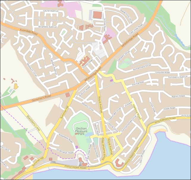
OpenStreetMap does not use a standard format such as shapefiles to store its data. Instead, it has developed its own XML-based format for representing geospatial data in the form of nodes (single points), ways (sequences of points that define a line), areas (closed ways that represent polygons), and relations (collections of other elements). Any element (node, way, or relation) can have a number of tags associated with it that provide additional information about that element.
The following is an example of what the OpenStreetMap XML data looks like:
<osm>
  <node id="603279517" lat="-38.1456457"
   lon="176.2441646".../>
  <node id="603279518" lat="-38.1456583"
   lon="176.2406726".../>
  <node id="603279519" lat="-38.1456540"
   lon="176.2380553".../>
  ...
  <way id="47390936"...>
    <nd ref="603279517"/>
    <nd ref="603279518"/>
    <nd ref="603279519"/>
    <tag k="highway" v="residential"/>
    <tag k="name" v="York Street"/>
  </way>
  ...
  <relation id="126207"...>
    <member type="way" ref="22930719" role=""/>
    <member type="way" ref="23963573" role=""/>
    <member type="way" ref="28562757" role=""/>
    <member type="way" ref="23963609" role=""/>
    <member type="way" ref="47475844" role=""/>
    <tag k="name" v="State Highway 30A"/>
    <tag k="ref" v="30A"/>
    <tag k="route" v="road"/>
    <tag k="type" v="route"/>
  </relation>
</osm>You can obtain geospatial data from OpenStreetMap in one of three ways:
- You can use the OpenStreetMap API to download a subset of the data you are interested in.
- You can download the entire OpenStreetMap database, called
Planet.osm, and process it locally. Note that this is a multi-gigabyte download. - You can make use of one of the mirror sites that provide OpenStreetMap data nicely packaged into smaller chunks and converted into other data formats. For example, you can download the data for North America on a state-by-state basis and in various formats, including shapefiles.
Let's take a closer look at each of these three options.
OpenStreetMap provides two APIs you can use:
- The Editing API (http://wiki.openstreetmap.org/wiki/API) can be used to retrieve and make changes to the OpenStreetMap dataset
- The Overpass API (http://wiki.openstreetmap.org/wiki/Overpass_API) provides a read-only interface to OpenStreetMap data
The Overpass API is most useful for retrieving data. It provides a sophisticated query language that you can use to obtain OpenStreetMap XML data based on the search criteria you specify. For example, you can retrieve a list of primary roads within a given bounding box using the following query:
way[highway=primary](-38.18, 176.13, -38.03, 176.38);out;
Using the python-overpy library (https://github.com/DinoTools/python-overpy), you can directly call the Overpass API from within your Python programs.
If you wish to download all of OpenStreetMap for processing on your computer, you will need to download the entire Planet.osm database. This database is available in two formats: a compressed XML-format file containing all the nodes, ways, and relations in the OpenStreetMap database, or a special binary format called PBF that contains the same information but is smaller and faster to read.
The Planet.osm database is currently 44 GB if you download it in compressed XML format or 29 GB if you download it in PBF format. Both formats can be downloaded from http://planet.openstreetmap.org.
The entire dump of the Planet.osm database is updated weekly, but diff files are created every week, day, hour, and minute. You can use these to update your existing copy of the Planet.osm database without having to download everything again.
Because of the size of the download, OpenStreetMap recommends that you use a mirror site rather than downloading Planet.osm directly from their servers. Extracts are also provided, which allow you to download the data for a given area rather than the entire world. These mirror sites and extracts are maintained by third parties; for a list of the URLs, refer to http://wiki.openstreetmap.org/wiki/Planet.osm.
Note that these mirrors and extracts are often available in alternative formats, including shapefiles and direct database dumps.
When you download Planet.osm, you will end up with an enormous file on your hard disk—currently, it is 576 GB if you download the data in XML format. You have two main options for processing this file using Python:
- You could use a Python library such as
imposm.parser(http://imposm.org/docs/imposm.parser/latest) to read through the file and extract the information you want - You could import the data into a database and then access that database from Python
In most cases, you will want to import the data into a database before you attempt to work with it. To do this, use the excellent
osm2pgsql tool, which is available at http://wiki.openstreetmap.org/wiki/Osm2pgsql. osm2pgsql was created to import the entire Planet.osm data into a PostgreSQL database and is therefore highly optimized for this task.
Once you have imported the Planet.osm data into a database on your computer, you can use the psycopg2 library, as described in Chapter 6, Spatial Databases, to access the OpenStreetMap data from your Python programs.
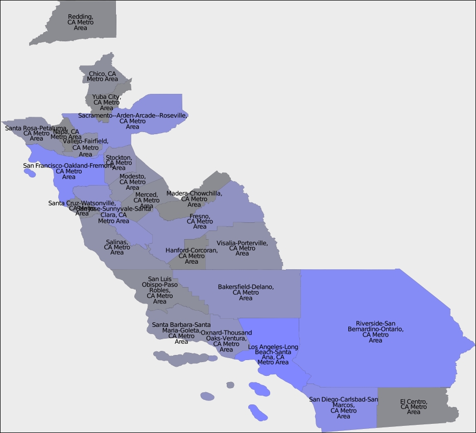
The United States Census Bureau have made available a large amount of geospatial data under the name TIGER (short for Topologically Integrated Geographic Encoding and Referencing System). The TIGER data includes information on streets, railways, rivers, lakes, geographic boundaries, legal and statistical areas such as school districts, and urban regions. Separate cartographic boundary and demographic files are also available for download.
The following diagram shows state and urban area outlines for California, based on data downloaded from the TIGER web site:
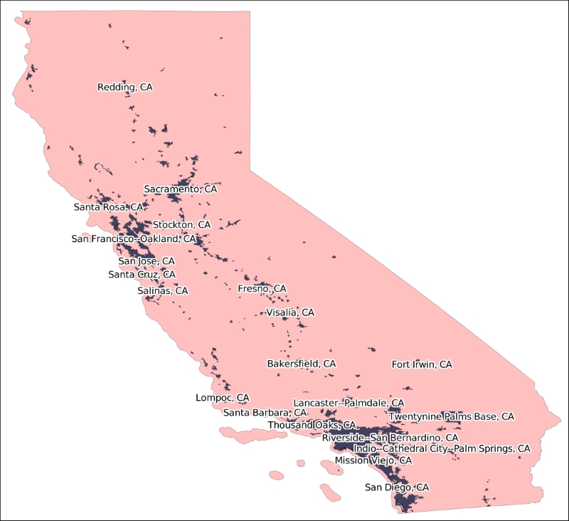
Because it is produced by the US government, TIGER only includes information for the United States and its protectorates (Puerto Rico, American Samoa, the Northern Mariana Islands, Guam, and the US Virgin Islands). For these areas, TIGER is an excellent source of geospatial data.
Up until 2006, the US Census Bureau provided TIGER data in a custom text-based format called TIGER/Line. TIGER/Line files stored each type of record in a separate file and required custom tools to process. Fortunately, OGR supports TIGER/Line files, should you need to read them.
Since 2007, all TIGER data has been produced in the form of shapefiles, which are (somewhat confusingly) called TIGER/Line shapefiles.
You can download up-to-date shapefiles containing geospatial data such as street address ranges, landmarks, census blocks, metropolitan statistical areas, and school districts. For example, the Core Based Statistical Area shapefile contains the outline of each metropolitan and micropolitan area in the US:
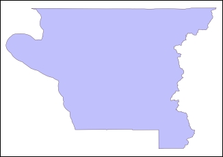
This particular feature has the following metadata associated with it:
|
Attribute name |
Value |
|---|---|
|
ALAND |
2606282680.0 |
|
AWATER |
578761025.0 |
|
CBSAFP |
18860 |
|
CSAFP |
None |
|
GEOID |
18860 |
|
INTPTLAT |
+41.7499033 |
|
INTPTLON |
-123.9809983 |
|
LSAD |
M2 |
|
MEMI |
2 |
|
MTFCC |
G3110 |
|
NAME |
Crescent City, CA |
|
NAMELSAD |
Crescent City, CA Micro Area |
Information on these various attributes can be found in the extensive documentation available on the TIGER web site.
You can also download shapefiles that include demographic data, such as population, number of houses, median age, and racial breakdown. For example, the following map tints each metropolitan area in California according to its total population as recorded in the latest (2010) census:
The TIGER data files can be downloaded from http://www.census.gov/geo/maps-data/data/tiger.html.
Make sure that you download the technical documentation, as it describes the various files you can download and all the attributes associated with each feature. For example, if you want to download the current set of urban areas for the US, the shapefile you are looking for is in a ZIP archive named tl_2015_us_uac10.zip and includes information such as the city or town name and the size of the urban area in square meters.
Natural Earth (http://www.naturalearthdata.com) is a web site that provides public-domain vector and raster map data at high, medium, and low resolutions. Two types of vector map data are provided:
- Cultural map data: This includes polygons for country, state or province, urban areas, and park outlines as well as point and line data for populated places, roads, and railways:
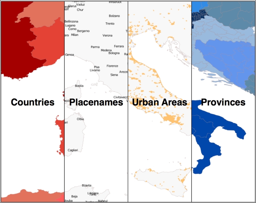
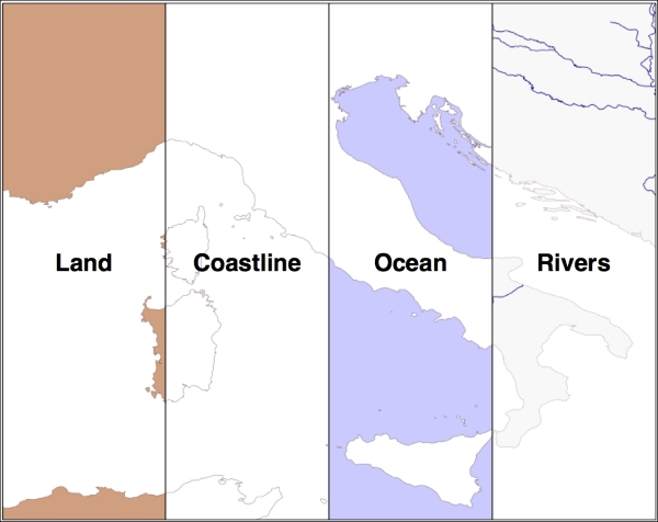
- Physical map data: This includes polygons and linestrings for land masses, coastlines, oceans, minor islands, reefs, rivers, lakes, and so on
All of this can be downloaded and used freely in your geospatial programs, making the Natural Earth site an excellent source of data for your application.
All the vector-format data on the Natural Earth web site is provided in the form of shapefiles. All the data is in geographic (latitude and longitude) coordinates, using the standard WGS84 datum, making it very easy to use these files in your own application.
The Natural Earth site is uniformly excellent, and downloading the files you want is easy: simply click on the Get the Data link on the main page. You can then choose the resolution and type of data you are looking for. You can also choose to download either a single shapefile or a number of shapefiles all bundled together. Once they have been downloaded, you can use the Python libraries discussed in the previous chapter to work with the contents of those shapefiles.
The Natural Earth web site is very comprehensive; it includes detailed information about the geospatial data you can download and a forum where you can ask questions and discuss any problems you may have.
The US National Geophysical Data Center (part of the NOAA) provides high-quality vector shoreline data for the entire world in the form of a database called the Global Self-consistent, Hierarchical, High-resolution Geography Database (GSHHG). This database includes detailed vector data for shorelines, lakes, and rivers in five different resolutions. The data has been broken out into four different levels: ocean boundaries, lake boundaries, island-in-lake boundaries, and pond-on-island-in-lake boundaries.
The following image shows European shorelines, lakes, and islands, taken from the GSHHG database:
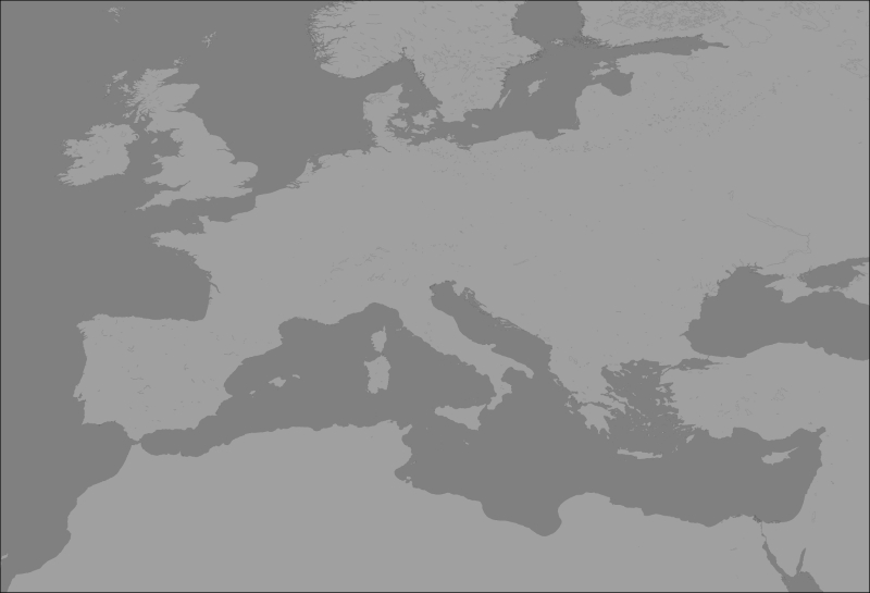
The GSHHG database has been constructed out of two public-domain geospatial databases: the World Data Bank II database includes data on coastlines, lakes, and rivers, while the World Vector Shorelines database only provides coastline data. Because the World Vector Shorelines database has more accurate data but lacks information on rivers and lakes, the two databases were combined to provide the most accurate information possible. After merging the databases, the author manually edited the data to make it consistent and remove a number of errors. The result is a high-quality database of land and water boundaries worldwide.
Note
More information about the process used to create the GSHHG database can be found at http://www.soest.hawaii.edu/pwessel/papers/1996/JGR_96/jgr_96.html
The GSHHG database can be downloaded in Shapefile format, among others. If you download the data in Shapefile format, you will end up with a total of twenty separate shapefiles, one for every combination of resolution and level:
- The resolution represents the amount of detail in the map:
Value
Resolution
Includes
cCrude
Features greater than 500 sq. km.
lLow
Features greater than 100 sq. km.
iIntermediate
Features greater than 20 sq. km.
hHigh
Features greater than 1 sq. km.
fFull
Every feature
- The level indicates the type of boundaries that are included in the shapefile:
Value
Includes
1Ocean boundaries
2Lake boundaries
3Island-in-lake boundaries
4Pond-on-island-in-lake boundaries
The name of the shapefile tells you the resolution and level of the included data. For example, the shapefile for ocean boundaries at full resolution would be named GSHHS_f_L1.shp.
Each shapefile consists of a single layer containing the various polygon features making up the given type of boundary.
The main GSHHG web site can be found at http://www.ngdc.noaa.gov/mgg/shorelines/gshhs.html.
Follow the download link on this page to see the list of files you can download. To download the data in shapefile format, you will want a file with a name like gshhg-shp-2.3.4.zip, where 2.3.4 is the version number of the database you are downloading.
Once you have downloaded and decompressed the file, you can extract the data from the individual shapefiles using OGR, as described in the previous chapter.
Many of the data sources we have examined so far are rather complex. If all you are looking for is some simple vector data covering the entire world, the World Borders Dataset may be all you need. While some of the country borders are apparently disputed, the simplicity of the World Borders Dataset makes it an attractive choice for many basic geospatial applications.
The following map was generated using the World Borders Dataset:
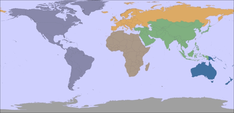
The World Borders Dataset will be used extensively throughout this book. Indeed, you have already seen an example program in Chapter 3, Python Libraries for Geospatial Development, where we used Mapnik to generate a world map using the World Borders Dataset shapefile.
The World Borders Dataset is available in the form of a shapefile with a single layer, with one feature for each country. For each country, the corresponding feature has one or more polygons that define the country's boundary along with useful attributes, including the name of the country or area; various ISO, FIPS, and UN codes identifying the country; a region and subregion classification; and the country's population, land area, and latitude/longitude.
The various codes make it easy to match the features against your own country-specific data, and you can also use information such as the population and area to highlight different countries on the map. For example, the preceding map used the region field to draw each geographic region in a different color.
The World Borders Dataset can be downloaded from http://thematicmapping.org/downloads/world_borders.php.
This web site also provides more details about the contents of the dataset, including links to the United Nations' site where the region and subregion codes are listed.