One of the older techniques designed to frustrate the disassembly process involves the creative use of instructions and data to prevent the disassembly from finding the correct starting address for one or more instructions. Forcing the disassembler to lose track of itself in this manner usually results in a failed or, at a minimum, incorrect disassembly listing.

The following listing shows IDA’s efforts to disassemble a portion of the Shiva^[149] anti–reverse engineering tool:

LOAD:0A04B0D1                 call  near ptr loc_A04B0D6+1
  LOAD:0A04B0D6
  LOAD:0A04B0D6 loc_A04B0D6:                      ; CODE XREF: start+11↓p
 LOAD:0A04B0D6                 mov     dword ptr [eax-73h], 0FFEB0A40h
  LOAD:0A04B0D6 start           endp
  LOAD:0A04B0D6
  LOAD:0A04B0DD
  LOAD:0A04B0DD loc_A04B0DD:                      ; CODE XREF: LOAD:0A04B14C↓j
  LOAD:0A04B0DD                 loopne  loc_A04B06F
  LOAD:0A04B0DF                 mov     dword ptr [eax+56h], 5CDAB950h
 LOAD:0A04B0E6                 iret
  LOAD:0A04B0E6 ;---------------------------------------------------------------
 LOAD:0A04B0E7                 db 47h
  LOAD:0A04B0E8                 db 31h, 0FFh, 66h
    LOAD:0A04B0EB ;---------------------------------------------------------------
  LOAD:0A04B0EB
  LOAD:0A04B0EB loc_A04B0EB:                      ; CODE XREF: LOAD:0A04B098↑j
  LOAD:0A04B0EB                 mov     edi, 0C7810D98h

This example executes a call (a jump can just as easily be used) into the middle of an existing instruction . Since the function call is assumed to return, the succeeding instruction at address 0A04B0D6 is disassembled (incorrectly). The actual target of the call instruction, loc_A04B0D6+1 (0A04B0D7), cannot be disassembled because the associated bytes have already been incorporated into the 5-byte instruction at 0A04B0D6. Assuming we notice that this is taking place, the remainder of the disassembly must be considered suspect. Evidence of this fact shows up in the form of unexpected user-space instructions (in this case an iret^[150]) and miscellaneous databytes .

Note that this type of behavior is not restricted to IDA. Virtually all disassemblers, whether they utilize a recursive descent algorithm or a linear sweep algorithm, fall victim to this technique.

The proper way to deal with this situation in IDA is to undefine the instruction that contains the bytes that are the target of the call and then define an instruction at the call target address in an attempt to resynchronize the disassembly. Of course, the use of an interactive disassembler greatly simplifies this process. Using IDA, a quick Edit ▸ Undefine (hotkey U) with the cursor positioned at followed by an Edit ▸ Code (hotkey C) with the cursor repositioned on address 0A04B0D7 results in the listing shown here:

LOAD:0A04B0D1                 call    loc_A04B0D7
  LOAD:0A04B0D1 ;------------------------------------------------------------
 LOAD:0A04B0D6                 db 0C7h ; ¦
  LOAD:0A04B0D7 ;------------------------------------------------------------
  LOAD:0A04B0D7
  LOAD:0A04B0D7 loc_A04B0D7:                   ; CODE XREF: start+11↑p
 LOAD:0A04B0D7                 pop     eax
  LOAD:0A04B0D8                 lea     eax, [eax+0Ah]
  LOAD:0A04B0DB
  LOAD:0A04B0DB loc_A04B0DB:                   ; CODE XREF: start:loc_A04B0DB↑j
 LOAD:0A04B0DB                 jmp     short near ptr loc_A04B0DB+1
  LOAD:0A04B0DB start           endp
  LOAD:0A04B0DB
  LOAD:0A04B0DB ;------------------------------------------------------------
  LOAD:0A04B0DD                 db 0E0h ; a

At this point, it is somewhat more obvious that the byte at address 0A04B0D6 is never executed. The instruction at 0A04B0D7 (the target of the call) is used to clear the return address (from the bogus call) off the stack, and execution continues. Note that is does not take long before the technique is used again, this time using a 2-byte jump instruction at address 0A04B0DB , which actually jumps into the middle of itself. Here again, we are obligated to undefine an instruction in order to get to the start of the next instruction. One more application of the undefine (at 0A04B0DB) and redefine (at 0A04B0DC) processes yields the following disassembly:

 LOAD:0A04B0D7                 pop     eax
 LOAD:0A04B0D8                 lea     eax, [eax+0Ah]
  LOAD:0A04B0D8 ; --------------------------------------------------------------
  LOAD:0A04B0DB                 db 0EBh ; d
  LOAD:0A04B0DC ; --------------------------------------------------------------
 LOAD:0A04B0DC                 jmp     eax
  LOAD:0A04B0DC start           endp

The target of the jump instruction turns out to be yet another jump instruction . In this case, however, the jump is impossible for a disassembler (and potentially confusing to the human analyst) to follow, as the target of the jump is contained in a register (EAX) and computed at runtime. This is an example of another type of anti–static analysis technique, discussed in Dynamically Computed Target Addresses in Dynamically Computed Target Addresses. In this case the value contained in the EAX register is not difficult to determine given the relatively simple instruction sequence that precedes the jump. The pop instruction at loads the return address from the call instruction in the previous example (0A04B0D6) into the EAX register, while the following instruction has the effect of adding 10 to EAX. Thus the target of the jump instruction is 0A04B0E0, and this is the address at which we must resume the disassembly process.

The final example of desynchronization taken from a different binary demonstrates how processor flags may be utilized to turn conditional jumps into absolute jumps. The following disassembly demonstrates the use of the x86 Z flag for just such a purpose:

 .text:00401000                 xor     eax, eax
 .text:00401002                 jz      short near ptr loc_401009+1
 .text:00401004                 mov     ebx, [eax]
 .text:00401006                 mov     [ecx-4], ebx
  .text:00401009
  .text:00401009 loc_401009:                     ; CODE XREF: .text:00401002↑j
 .text:00401009                 call    near ptr 0ADFEFFC6h
  .text:0040100E                 ficom   word ptr [eax+59h]

Here, the xor instruction is used to zero the EAX register and set the x86 Z flag. The programmer, knowing that the Z flag is set, utilizes a jump-on-zero (jz) instruction , which will always be taken, to attain the effect of an unconditional jump. As a result, the instructions and between the jump and the jump target will never be executed and serve only to confuse any analyst who fails to realize this fact. Note that, once again, this example obscures the actual jump target by jumping into the middle of an instruction . Properly disassembled, the code should read as follows:

.text:00401000                 xor     eax, eax
  .text:00401002                 jz      short loc_40100A
  .text:00401004                 mov     ebx, [eax]
  .text:00401006                 mov     [ecx-4], ebx
  .text:00401006 ; -------------------------------------------------------------
 .text:00401009                 db 0E8h ; F
  .text:0040100A ; -------------------------------------------------------------
  .text:0040100A
  .text:0040100A loc_40100A:                     ; CODE XREF: .text:00401002↑j
 .text:0040100A                 mov     eax, 0DEADBEEFh
  .text:0040100F                 push    eax
  .text:00401010                 pop     ecx

The actual target of the jump has been revealed, as has the extra byte that caused the desynchronization in the first place. It is certainly possible to use far more roundabout ways of setting and testing flags prior to executing a conditional jump. The level of difficulty for analyzing such code increases with the number of operations that may affect the CPU flag bits prior to testing their value.

Do not confuse the title of this section with an anti–dynamic analysis technique. The phrase dynamically computed simply means that an address to which execution will flow is computed at runtime. In this section we discuss several ways in which such an address can be derived. The intent of such techniques is to hide (obfuscate) the actual control flow path that a binary will follow from the prying eyes of the static analysis process.

One example of this technique was shown in the preceding section. The example used a call statement to place a return address on the stack. The return address was popped directly off the stack into a register, and a constant value was added to the register to derive the final target address, which was ultimately reached by performing a jump to the location specified by the register contents.

An infinite number of similar code sequences can be developed for deriving a target address and transferring control to that address. The following code, which wraps up the initial startup sequence in Shiva, demonstrates an alternate method for dynamically computing target addresses:

LOAD:0A04B3BE                 mov     ecx, 7F131760h  ; ecx = 7F131760
  LOAD:0A04B3C3                 xor     edi, edi        ; edi = 00000000
  LOAD:0A04B3C5                 mov     di, 1156h       ; edi = 00001156
  LOAD:0A04B3C9                 add     edi, 133AC000h  ; edi = 133AD156
  LOAD:0A04B3CF                 xor     ecx, edi        ; ecx = 6C29C636
    LOAD:0A04B3D1                 sub     ecx, 622545CEh  ; ecx = 0A048068
  LOAD:0A04B3D7                 mov     edi, ecx        ; edi = 0A048068
  LOAD:0A04B3D9                 pop     eax
  LOAD:0A04B3DA                 pop     esi
  LOAD:0A04B3DB                 pop     ebx
  LOAD:0A04B3DC                 pop     edx
  LOAD:0A04B3DD                 pop     ecx
 LOAD:0A04B3DE                 xchg    edi, [esp]      ; TOS = 0A048068
  LOAD:0A04B3E1                 retn                    ; return to 0A048068

The comments in the right-hand margin document the changes being made to various CPU registers at each instruction. The process culminates in a derived value being moved into the top position of the stack (TOS) , which causes the return instruction to transfer control to the computed location (0A048068 in this case). Code sequences such as these can significantly increase the amount of work that must be performed during static analysis, as the analyst must essentially run the code by hand to determine the actual control flow path taken in the program.

Much more complex types of control flow hiding have been developed and utilized in recent years. In the most complex cases, a program will use multiple threads or child processes to compute control flow information and receive that information via some form of interprocess communication (for child processes) or synchronization primitives (for multiple threads). In such cases, static analysis can become extremely difficult, as it becomes necessary to understand not only the behavior of multiple executable entities but also the exact manner by which those entities exchange information. For example, one thread may wait on a shared semaphore^[151] object, while a second thread computes values or modifies code that the first thread will make use of once the second thread signals its completion via the semaphore.

Another technique, frequently used within Windows-oriented malware, involves configuring an exception handler,^[152] intentionally triggering an exception, and then manipulating the state of the process’s registers while handling the exception. The following example is used by the tElock anti–reverse engineering tool to obscure the program’s actual control flow:

 .shrink:0041D07A        call    $+5
 .shrink:0041D07F        pop     ebp
 .shrink:0041D080        lea     eax, [ebp+46h]  ; eax holds 0041D07F + 46h
  .shrink:0041D081        inc     ebp
 .shrink:0041D083        push    eax
  .shrink:0041D084        xor     eax, eax
 .shrink:0041D086        push    dword ptr fs:[eax]
 .shrink:0041D089        mov     fs:[eax], esp
 .shrink:0041D08C        int     3               ; Trap to Debugger
  .shrink:0041D08D        nop
  .shrink:0041D08E        mov     eax, eax
  .shrink:0041D090        stc
  .shrink:0041D091        nop
  .shrink:0041D092        lea     eax, ds:1234h[ebx*2]
  .shrink:0041D099        clc
  .shrink:0041D09A        nop
  .shrink:0041D09B        shr     ebx, 5
  .shrink:0041D09E        cld
  .shrink:0041D09F        nop
  .shrink:0041D0A0        rol     eax, 7
  .shrink:0041D0A3        nop
  .shrink:0041D0A4        nop
 .shrink:0041D0A5        xor     ebx, ebx
 .shrink:0041D0A7        div     ebx             ; Divide by zero
  .shrink:0041D0A9        pop     dword ptr fs:0

The sequence begins by using a call to the next instruction ; the call instruction pushes 0041D07F onto the stack as a return address, which is promptly popped off the stack into the EBP register . Next , the EAX register is set to the sum of EBP and 46h, or 0041D0C5, and this address is pushed onto the stack as the address of an exception handler function. The remainder of the exception handler setup takes place at and , which complete the process of linking the new exception handler into the existing chain of exception handlers referenced by fs:[0].^[153] The next step is to intentionally generate an exception , in this case an int 3, which is a software trap (interrupt) to the debugger. In x86 programs, the int 3 instruction is used by debuggers to implement a software breakpoint. Normally at this point, an attached debugger would gain control; in fact, if a debugger is attached, it will have the first opportunity to handle the exception, thinking that it is a breakpoint. In this case, the program fully expects to handle the exception, so any attached debugger must be instructed to pass the exception along to the program. Failing to allow the program to handle the exception may result in an incorrect operation and possibly a crash of the program. Without understanding how the int 3 exception is handled, it is impossible to know what may happen next in this program. If we assume that execution simply resumes following the int 3, then it appears that a divide-by-zero exception will eventually be triggered by instructions and .

The exception handler associated with the preceding code begins at address 0041D0C5. The first portion of this function is shown here:

.shrink:0041D0C5 sub_41D0C5      proc near     ; DATA XREF: .stack:0012FF9C↑o
  .shrink:0041D0C5
  .shrink:0041D0C5 pEXCEPTION_RECORD  = dword ptr  4
  .shrink:0041D0C5 arg_4               = dword ptr  8
 .shrink:0041D0C5 pCONTEXT            = dword ptr  0Ch
    .shrink:0041D0C5
 .shrink:0041D0C5        mov     eax, [esp+pEXCEPTION_RECORD]
 .shrink:0041D0C9        mov     ecx, [esp+pCONTEXT]  ; Address of SEH CONTEXT
 .shrink:0041D0CD        inc     [ecx+CONTEXT._Eip]   ; Modify saved eip
 .shrink:0041D0D3        mov     eax, [eax]           ; Obtain exception type
 .shrink:0041D0D5        cmp     eax, EXCEPTION_INT_DIVIDE_BY_ZERO
  .shrink:0041D0DA        jnz     short loc_41D100
  .shrink:0041D0DC        inc     [ecx+CONTEXT._Eip]   ; Modify eip again
 .shrink:0041D0E2
        xor     eax, eax             ; Zero x86 debug registers
  .shrink:0041D0E4        and     [ecx+CONTEXT.Dr0], eax
  .shrink:0041D0E7        and     [ecx+CONTEXT.Dr1], eax
  .shrink:0041D0EA        and     [ecx+CONTEXT.Dr2], eax
  .shrink:0041D0ED        and     [ecx+CONTEXT.Dr3], eax
  .shrink:0041D0F0        and     [ecx+CONTEXT.Dr6], 0FFFF0FF0h
  .shrink:0041D0F7        and     [ecx+CONTEXT.Dr7], 0DC00h
  .shrink:0041D0FE        jmp     short locret_41D160

The third argument to the exception handler function is a pointer to a Windows CONTEXT structure (defined in the Windows API header file winnt.h). The CONTEXT structure is initialized with the contents of all CPU registers as they existed at the time of the exception. An exception handler has the opportunity to inspect and, if desired, modify the contents of the CONTEXT structure. If the exception handler feels that it has corrected the problem that led to the exception, it can notify the operating system that the offending thread should be allowed to continue. At this point the operating system reloads the CPU registers for the thread from the CONTEXT structure that was provided to the exception handler, and execution of the thread resumes as if nothing had ever happened.

In the preceding example, the exception handler begins by accessing the thread’s CONTEXT in order to increment the instruction pointer , thus moving beyond the instruction that generated the exception. Next, the exception’s type code (a field within the provided EXCEPTION_RECORD ) is retrieved in order to determine the nature of the exception. This portion of the exception handler deals with the divide-by-zero error , generated in the previous example, by zeroing all of the x86 hardware debugging registers.^[154] Without examining the remainder of the tElock code, it is not immediately apparent why the debug registers are being cleared. In this case, tElock is clearing values from a previous operation in which it used the debug registers to set four breakpoints in addition to the int 3 seen previously. In addition to obfuscating the true flow of the program, clearing or modifying the x86 debug registers can wreak havoc with software debuggers such as OllyDbg or IDA’s own internal debugger. Such anti-debugging techniques are discussed in Anti–Dynamic Analysis Techniques in Anti–Dynamic Analysis Techniques.

Opcode Obfuscation

While the techniques described to this point may provide—in fact, are intended to provide—a hindrance to understanding a program’s control flow, none prevent you from observing the correct disassembled form of a program you are analyzing. Desynchronization had the greatest impact on the disassembly, but it was easily defeated by reformatting the disassembly to reflect the correct instruction flow.

A more effective technique for preventing correct disassembly is to encode or encrypt the actual instructions when the executable file is being created. The obfuscated instructions are useless to the CPU and must be de-obfuscated back to their original form before they are fetched for execution by the CPU. Therefore, at least some portion of the program must remain unencrypted in order to serve as the startup routine, which, in the case of an obfuscated program, is usually responsible for de-obfuscating some or all of the remainder of the program. A very generic overview of the obfuscation process is shown in Figure 21-1.

Figure 21-1. Generic obfuscation process

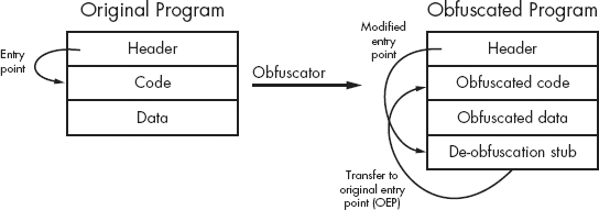
As shown, the input to the process is a program that a user wishes to obfuscate for some reason. In many cases, the input program is written using standard programming languages and build tools (editors, compilers, and the like) with little thought required about the obfuscation to come. The resulting executable file is fed into an obfuscation utility, which transforms the binary into a functionally equivalent, yet obfuscated, binary. As depicted, the obfuscation utility is responsible for obfuscating the original program’s code and data sections and adding additional code (a de-obfuscation stub) that performs the task of de-obfuscating the code and data before the original functionality can be accessed at runtime. The obfuscation utility also modifies the program headers to redirect the program entry point to the de-obfuscation stub, ensuring that execution begins with the de-obfuscation process. Following de-obfuscation, execution typically transfers to the entry point of the original program, which begins execution as if it had never been obfuscated at all.

This oversimplified process varies widely based on the obfuscation utility that is used to create the obfuscated binary. An ever-increasing number of utilities are available to handle the obfuscation process. Such utilities offer features ranging from compression to anti-disassembly and anti-debugging techniques. Examples include programs such as UPX^[155] (compressor, also works with ELF), ASPack^[156] (compressor), ASProtect (anti–reverse engineering by the makers of ASPack), and tElock^[157] (compression and anti–reverse engineering) for Windows PE files, and Burneye^[158] (encryption) and Shiva^[159] (encryption and anti-debugging) for Linux ELF binaries. The capabilities of obfuscation utilities have advanced to the point that some anti–reverse engineering tools such as WinLicense^[160] provide more integration throughout the entire build process, allowing programmers to integrate anti–reverse engineering features at every step, from source code through post-processing the compiled binary file.

A more recent evolution in the world of obfuscation programs involves wrapping the original executable with a virtual machine execution engine. Depending on the sophistication of the virtualizing obfuscator, the original machine code may never execute directly; instead that code is interpreted by a byte code–oriented virtual machine. Very sophisticated virtualizers are capable of generating unique virtual machine instances each time they run, making it difficult to create an all-purpose de-obfuscation algorithm to defeat them. VMProtect^[161] is one example of a virtualizing obfuscator. VMProtect was used to obfuscate the Clampi^[162] trojan.

As with any offensive technology, defensive measures have been developed to counter many anti–reverse engineering tools. In most cases the goal of such tools is to recover the original, unprotected executable file (or a reasonable facsimile), which can then be analyzed using more traditional tools such as disassemblers and debuggers. One such tool designed to de-obfuscate Windows executables is called QuickUnpack.^[163] QuickUnpack, like many other automated unpackers, operates by functioning as a debugger and allowing an obfuscated binary to execute through its de-obfuscation phase and then capturing the process image from memory. Beware that this type of tool actually runs potentially malicious programs in the hope of intercepting the execution of those programs after they have unpacked or de-obfuscated themselves but before they have a chance to do anything malicious. Thus, you should always execute such programs in a sandbox-type environment.

Using a purely static analysis environment to analyze obfuscated code is a challenging task at best. Without being able to execute the de-obfuscation stub, some means of unpacking or decrypting the obfuscated portions of the binary must be employed before disassembly of the obfuscated code can begin. Figure 21-2 shows the layout of an executable that has been packed using the UPX packer. The only portion of the address space that IDA has identified as code is the thin stripe at , which happens to be the UPX decompression stub.

Figure 21-2. IDA navigation band for a binary packed using UPX

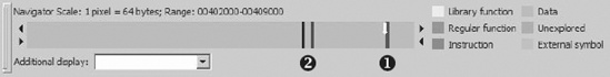
Examination of the contents of the address space would reveal empty space to the left of and apparently random data in the region between and . The random data is the result of the UPX compression process, and the job of the decompression stub is to unpack that data into the empty region at the left of the navigation band before finally transferring control to the unpacked code. Note that the unusual appearance of the navigation band is a potential tip-off that this binary has been obfuscated in some manner. In fact, a number of things typically stand out when viewing an obfuscated binary with IDA. Some potential tip-offs that a binary is obfuscated include the following:

• Very little code is highlighted in the navigation band.

• Very few functions are listed in the Functions window. Often only the start function will appear.

• Very few imported functions are listed in the Imports window.

• Very few legible strings appear in the Strings window (not opened by default). Often only the names of the few imported libraries and functions will be visible.

• One or more program sections will be both writable and executable.

• Nonstandard section names such as UPX0 or .shrink are used.

SANDBOX ENVIRONMENTS

The purpose of a sandbox environment for reverse engineering is to allow you to execute a program in a manner that allows observation of the program’s behavior without allowing that behavior to adversely impact critical components of your reverse engineering platform. Sandbox environments are commonly constructed using platform virtualization software such asd VMware,^[164] but they may be constructed on dedicated systems that are capable of being restored to a known good state following the execution of any malware.

A common feature of sandbox systems is the fact that they are typically heavily instrumented in order to observe and collect information on the behavior of programs run within the sandbox. Collected data may include information on the file system activity of a program, on the registry activity of a (Windows) program, and about any networking activity generated by the program.

The information presented in the navigation band can be correlated with the properties of each segment within the binary to determine whether the information presented in each display is consistent. The segments listing for this binary is shown here:

Name   Start    End      R W X D L Align Base Type   Class
 UPX0   00401000 00407000 R W X . L para  0001 public CODE
 UPX1   00407000 00409000 R W X . L para  0002 public CODE
  UPX2   00409000 0040908C R W . . L para  0003 public DATA
  .idata 0040908C 004090C0 R W . . L para  0003 public XTRN
  UPX2   004090C0 0040A000 R W . . L para  0003 public DATA

In this case, the entire range of addresses comprising segment UPX0 and segment UPX1 (00401000-00409000) is marked as executable (the X flag is set). Given this fact, we should expect to see the entire navigation band colorized to represent code. The fact that we do not, coupled with the fact that inspection reveals the entire range of UPX0 to be empty, should be considered highly suspicious. Within IDA, the section header for UPX0 contains the following lines:

UPX0:00401000 ;  Section 1. (virtual address 00001000)
UPX0:00401000 ;  Virtual size                  : 00006000 (  24576.)
UPX0:00401000 ;Section size in file          : 00000000 (      0.)
UPX0:00401000 ;  Offset to raw data for section: 00000200
UPX0:00401000 ;Flags E0000080: Bss Executable Readable Writable

Techniques for using IDA to perform the decompression operation in a static context (without actually executing the binary) are discussed in Static De-obfuscation of Binaries Using IDA in Static De-obfuscation of Binaries Using IDA.

In order to avoid leaking information about potential actions that a binary may perform, an additional anti–static analysis technique is aimed at making it difficult to determine which shared libraries and library functions are used within an obfuscated binary. In most cases, it is possible to render tools such as dumpbin, ldd, and objdump ineffective for the purposes of listing library dependencies.

The effect of such obfuscations on IDA is most obvious in the Imports window. The entire content of the Imports window for our earlier tElock example is shown here:

Address   Ordinal   Name                  Library
0041EC2E            GetModuleHandleA      kernel32
0041EC36            MessageBoxA           user32

Only two external functions are referenced, GetModulehandleA (from kernel32.dll) and MessageBoxA (from user32.dll). Virtually nothing about the behavior of the program can be inferred from this short list. How then does such a program get anything useful accomplished? Here again the techniques are varied, but they essentially boil down to the fact that the program itself must load any additional libraries that it depends on, and once the libraries are loaded, the program must locate any required functions within those libraries. In most cases, these tasks are performed by the de-obfuscation stub prior to transferring control to the de-obfuscated program. The end goal is for the program’s import table to have been properly initialized, just as if the process had been performed by the operating system’s own loader.

For Windows binaries, a simple approach is to use the LoadLibrary function to load required libraries by name and then perform function address lookups within each library using the GetProcAddress function. In order to use these functions, a program must be either explicitly linked to them or have an alternate means of looking them up. The Names listing for the tElock example does not include either of these functions, while the Names listing for the UPX example shown here includes both.

Address   Ordinal   Name                  Library
0040908C            LoadLibraryA          KERNEL32
00409090            GetProcAddress        KERNEL32
00409094            ExitProcess           KERNEL32
0040909C            RegCloseKey           ADVAPI32
004090A4            atoi                  CRTDLL
004090AC            ExitWindowsEx         USER32
004090B4            InternetOpenA         WININET
004090BC            recv                  wsock32

The actual UPX code responsible for rebuilding the import table is shown in Example 21-1.

UPX1:0040886C loc_40886C:                       ; CODE XREF: start+12E↓j
  UPX1:0040886C        mov     eax, [edi]
  UPX1:0040886E        or      eax, eax
  UPX1:00408870        jz      short loc_4088AE
  UPX1:00408872        mov     ebx, [edi+4]
  UPX1:00408875        lea     eax, [eax+esi+8000h]
  UPX1:0040887C        add     ebx, esi
  UPX1:0040887E        push    eax
  UPX1:0040887F        add     edi, 8
 UPX1:00408882        call    dword ptr [esi+808Ch] ; LoadLibraryA
  UPX1:00408888        xchg    eax, ebp
  UPX1:00408889
  UPX1:00408889 loc_408889:                       ; CODE XREF: start+146↓j
  UPX1:00408889        mov     al, [edi]
  UPX1:0040888B        inc     edi
  UPX1:0040888C        or      al, al
  UPX1:0040888E        jz      short loc_40886C
  UPX1:00408890        mov     ecx, edi
  UPX1:00408892        push    edi
  UPX1:00408893        dec     eax
  UPX1:00408894        repne scasb
  UPX1:00408896        push    ebp
 UPX1:00408897        call    dword ptr [esi+8090h] ; GetProcAddress
    UPX1:0040889D        or      eax, eax
  UPX1:0040889F        jz      short loc_4088A8
 UPX1:004088A1        mov     [ebx], eax            ; Save to import table
  UPX1:004088A3        add     ebx, 4
  UPX1:004088A6        jmp     short loc_408889

This example contains an outer loop responsible for calling LoadLibraryA^[165] and an inner loop responsible for calling GetProcAddress . Following each successful call to GetProcAddress, the newly retrieved function address is stored into the reconstructed import table .

These loops are executed as the last portion of the UPX de-obfuscation stub, because each function takes string pointer parameters that point to either a library name or a function name, and the associated strings are held within the compressed data region to avoid detection by the strings utility. As a result, library loading in UPX cannot take place until the required strings have been decompressed.

Returning to the tElock example, a different problem presents itself. With only two imported functions, neither of which is LoadLibraryA or GetProcAddress, how can the tElock utility perform the function-resolution tasks that were performed by UPX? All Windows processes depend on kernel32.dll, which means that it is present in memory for all processes. If a program can locate kernel32.dll, a relatively straightforward process may be followed to locate any function within the DLL, including LoadLibraryA and GetProcAddress. As shown previously, with these two functions in hand, it is possible to load any additional libraries required by the process and locate all required functions within those libraries. In his paper “Understanding Windows Shellcode,”^[166] Skape discusses techniques for doing exactly this. While tElock does not use the exact techniques detailed by Skape, there are many parallels, and the net effect is to obscure the details of the loading and linking process. Without carefully tracing the program’s instructions, it is extremely easy to overlook the loading of a library or the lookup of a function address. The following small code fragment illustrates the manner in which tElock attempts to locate the address of LoadLibraryA:

.shrink:0041D1E4                 cmp     dword ptr [eax], 64616F4Ch
.shrink:0041D1EA                 jnz     short loc_41D226
.shrink:0041D1EC                 cmp     dword ptr [eax+4], 7262694Ch
.shrink:0041D1F3                 jnz     short loc_41D226
.shrink:0041D1F5                 cmp     dword ptr [eax+8], 41797261h
.shrink:0041D1FC                 jnz     short loc_41D226

It is immediately obvious that several comparisons are taking place in rapid succession. What may not be immediately clear is the purpose of these comparisons. Reformatting the operands used in each comparison sheds a little light on the code, as seen here:

.shrink:0041D1E4                 cmp     dword ptr [eax], 'daoL'
.shrink:0041D1EA                 jnz     short loc_41D226
.shrink:0041D1EC                 cmp     dword ptr [eax+4], 'rbiL'
.shrink:0041D1F3                 jnz     short loc_41D226
.shrink:0041D1F5                 cmp     dword ptr [eax+8], 'Ayra'
.shrink:0041D1FC                 jnz     short loc_41D226

Each hexadecimal constant is actually a sequence of four ASCII characters, which taken in order (recall that the x86 is a little-endian processor and we need to read the characters in reverse order) spell LoadLibraryA. If the three comparisons succeed, then tElock has located the export table entry for LoadLibraryA, and in a few short operations, the address of this function will be obtained and available for use in loading additional libraries. An interesting characteristic of tElock’s approach to function lookup is that it is somewhat resistant to strings analysis because the 4-byte constants embedded directly in the program’s instructions do not look like more standard, null-terminated strings and thus do not get included in strings lists generated by IDA.

Manually reconstructing a program’s import table through careful analysis of the program’s code is made easier in the case of UPX and tElock because, ultimately, they both contain ASCII character data that we can use to determine exactly which libraries and which functions are being referenced. Skape’s paper details a function-resolution process in which no strings at all appear within the code. The basic idea discussed in the paper is to precompute a unique hash^[167] value for the name of each function that you need to resolve. To resolve each function, a search is conducted through a library’s exported names table. Each name in the table is hashed, and the resulting hash is compared against the precomputed hash value for the desired function. If the hashes match, the desired function has been located, and you can easily find its address in the library’s export address table. In order to statically analyze binaries obfuscated in this manner, you need to understand the hashing algorithm used for each function name and apply that algorithm to all of the names exported by the library that the program is searching. With a complete table of hashes in hand, you will be able to do a simple lookup of each hash that you encounter in the program to determine which function the hash references.^[168] A portion of such a table, generated for kernel32.dll, might look like this:

 GetProcAddress : 8A0FB5E2
  GetProcessAffinityMask : B9756EFE
  GetProcessHandleCount : B50EB87C
  GetProcessHeap : C246DA44
  GetProcessHeaps : A18AAB23
  GetProcessId : BE05ED07

Note that the hash values are specific to the hash function being used within a particular binary and are likely to vary from one binary to another. Using this particular table, if the hash value 8A0FB5E2 was encountered within a program, we could quickly determine that the program was attempting to look up the address of the GetProcAddress function.

Skape’s use of hash values to resolve function names was originally developed and documented for use in exploit payloads for Windows vulnerabilities; however, hash values have been adopted for use in obfuscated programs as well. The WinLicense obfuscation utility is one example that makes use of such hashing techniques to disguise its behavior.

A final note on import tables is that, interestingly, IDA is sometimes able to offer you a clue that something is not quite right with a program’s import table. Obfuscated Windows binaries often have sufficiently altered import tables that IDA will notify you that something seems out of the ordinary with such a binary. Figure 21-3 shows the warning dialog that IDA displays in such cases.

Figure 21-3. Mangled imports segment warning dialog

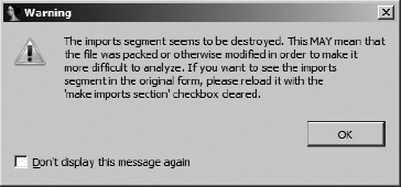
This dialog provides one of the earliest indications that a binary may have been obfuscated in some manner and should serve as a warning that the binary may be difficult to analyze. Thus, you should take care while analyzing the binary.

This category of anti–reverse engineering capability is mentioned only because of its unique potential to hinder reverse engineering efforts. Most reverse engineering tools can be viewed as highly specialized parsers that process input data to provide some sort of summary information or detail display. As software, these tools are not immune to the same types of vulnerabilities that affect all other software. Specifically, incorrect handling of user-supplied data may, in some cases, lead to exploitable conditions.

In addition to the techniques we have discussed thus far, programmers intent on preventing analysis of their software may opt for a more active form of anti–reverse engineering. By properly crafting input files, it may be possible to create a program that is both valid enough to execute properly and mal-formed enough to exploit a vulnerability in a reverse engineering tool. Such vulnerabilities, while uncommon, have been documented to include vulnerabilities in IDA.^[169] The goal of the attacker is to exploit the fact that a piece of malware is likely to get loaded into IDA at some point. At a minimum, the attacker may achieve a denial of service in which IDA always crashes before a database can be created; alternatively, the attacker may gain access to the analyst’s computer and associated network. Users concerned with this type of attack should consider performing all initial analysis tasks in a sandbox environment. For example, you might run a copy of IDA in a sandbox to create the initial database for all binaries. The initial database (which in theory is free from any malicious capability) can then be distributed to additional analysts, who need never touch the original binary file.