When you can find documentation on the format utilized by a particular file, your life will be significantly easier as you attempt to map the file into an IDA database. Example 18-1 shows the first few lines of a PE file loaded into IDA as a binary file. With no help from IDA, we turn to the PE specification,^[129] which states that a valid PE file will begin with a valid MS-DOS header structure. A valid MS-DOS header structure in turn begins with the 2-byte signature 4Dh 5Ah (MZ), which we see in the first two lines of Example 18-1.

At this point an understanding of the layout of an MS-DOS header is required. The PE specification would tell us that the 4-byte value located at offset 0x3C in the file indicates the offset to the next header we need to find—the PE header. Two strategies for breaking down the fields of the MS-DOS header are (1) to define appropriately sized data values for each field in the MS-DOS header or (2) to use IDA’s structure-creation facilities to define and apply an IMAGE_DOS_HEADER structure in accordance with the PE file specification.^[130] Using the latter approach would yield the following modified display:

seg000:00000000                 dw 5A4Dh                ; e_magic
seg000:00000000                 dw 90h                  ; e_cblp
seg000:00000000                 dw 3                    ; e_cp
seg000:00000000                 dw 0                    ; e_crlc
seg000:00000000                 dw 4                    ; e_cparhdr
seg000:00000000                 dw 0                    ; e_minalloc
seg000:00000000                 dw 0FFFFh               ; e_maxalloc
seg000:00000000                 dw 0                    ; e_ss
seg000:00000000                 dw 0B8h                 ; e_sp
seg000:00000000                 dw 0                    ; e_csum
seg000:00000000                 dw 0                    ; e_ip
seg000:00000000                 dw 0                    ; e_cs
seg000:00000000                 dw 40h                  ; e_lfarlc
seg000:00000000                 dw 0                    ; e_ovno
seg000:00000000                 dw 4 dup(0)             ; e_res
seg000:00000000                 dw 0                    ; e_oemid
seg000:00000000                 dw 0                    ; e_oeminfo
seg000:00000000                 dw 0Ah dup(0)           ; e_res2
seg000:00000000                 dd 80h                ; e_lfanew

The e_lfanew field has a value of 80h, indicating that a PE header should be found at offset 80h (128 bytes) into the database. Examining the bytes at offset 80h should reveal the magic number for a PE header, 50h 45h (PE), and allow us to build (based on our reading of the PE specification) and apply an IMAGE_NT_HEADERS structure at offset 80h into the database. A portion of the resulting IDA listing might look like the following:

seg000:00000080        dd 4550h        ; Signature
seg000:00000080        dw 14Ch       ; FileHeader.Machine
seg000:00000080        dw 4          ; FileHeader.NumberOfSections
seg000:00000080        dd 47826AB4h    ; FileHeader.TimeDateStamp
seg000:00000080        dd 0E00h        ; FileHeader.PointerToSymbolTable
seg000:00000080        dd 0FBh         ; FileHeader.NumberOfSymbols
seg000:00000080        dw 0E0h         ; FileHeader.SizeOfOptionalHeader
seg000:00000080        dw 307h         ; FileHeader.Characteristics
seg000:00000080        dw 10Bh         ; OptionalHeader.Magic
seg000:00000080        db 2            ; OptionalHeader.MajorLinkerVersion
seg000:00000080        db 38h          ; OptionalHeader.MinorLinkerVersion
seg000:00000080        dd 600h         ; OptionalHeader.SizeOfCode
seg000:00000080        dd 400h         ; OptionalHeader.SizeOfInitializedData
seg000:00000080        dd 200h         ; OptionalHeader.SizeOfUninitializedData
seg000:00000080        dd 1000h      ; OptionalHeader.AddressOfEntryPoint
seg000:00000080        dd 1000h        ; OptionalHeader.BaseOfCode
seg000:00000080        dd 0            ; OptionalHeader.BaseOfData
seg000:00000080        dd 400000h    ; OptionalHeader.ImageBase
seg000:00000080        dd 1000h      ; OptionalHeader.SectionAlignment
seg000:00000080        dd 200h       ; OptionalHeader.FileAlignment

The preceding listings and discussion bear many similarities to the exploration of MS-DOS and PE header structures conducted in Chapter 8. In this case, however, the file has been loaded into IDA without the benefit of the PE loader, and rather than being a curiosity as they were in Chapter 8, the header structures are essential to a successful understanding of the remainder of the database.

At this point, we have revealed a number of interesting pieces of information that will help us to further refine our database layout. First, the Machine field in a PE header indicates the target CPU type for which the file was built. In this example the value 14Ch indicates that the file is for use with x86 processor types. Had the machine type been something else, such as 1C0h (ARM), we would actually need to close the database and restart our analysis, making certain that we select the correct processor type in the initial loading dialog. Once a database has been loaded, it is not possible to change the processor type in use with that database.

The ImageBase field indicates the base virtual address for the loaded file image. Using this information, we can finally begin to incorporate some virtual address information into the database. Using the Edit ▸ Segments ▸ Rebase Program menu option, we can specify a new base address for the first segment of the program, as shown in Figure 18-2.

Figure 18-2. Specifying a new base address for a program

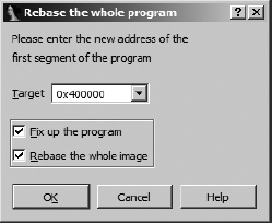
In the current example, only one segment exists, because IDA creates only one segment to hold the entire file when a file is loaded in binary mode. The two checkbox options shown in the dialog determine how IDA handles relocation entries when segments are moved and whether IDA should move every segment present in the database, respectively. For a file loaded in binary mode, IDA will not be aware of any relocation information. Similarly, with only one segment present in the program, the entire image will be rebased by default.

The AddressOfEntryPoint field specifies the relative virtual address (RVA) of the program entry point. An RVA is a relative offset from the program’s base virtual address, while the program entry point represents the address of the first instruction within the program that will be executed. In this case an entry point RVA of 1000h indicates that the program will begin execution at virtual address 401000h (400000h + 1000h). This is an important piece of information, because it is our first indication of where we should begin looking for code within the database. Before we can do that, however, we need to properly map the remainder of the database to appropriate virtual addresses.

The PE format makes use of sections to describe the mapping of file content to memory ranges. By parsing the section headers for each section in the file, we can complete the basic virtual memory layout of the database. The NumberOfSections field indicates the number of sections contained in a PE file; in this case there are four. Referring once again to the PE specification, we would learn that an array of section header structures immediately follows the IMAGE_NT_HEADERS structure. Individual elements in the array are IMAGE_SECTION_HEADER structures, which we could define in IDA’s Structures window and apply (four times in this case) to the bytes following the IMAGE_NT_HEADERS structure.

Before we discuss segment creation, two additional fields worth pointing out are FileAlignment and SectionAlignment . These fields indicate how the data for each section is aligned^[131] within the file and how that same data will be aligned when mapped into memory, respectively. In our example, each section is aligned to a 200h byte offset within the file; however, when loaded into memory, those same sections will be aligned on addresses that are multiples of 1000h. The smaller FileAlignment value offers a means of saving space when an executable image is stored in a file, while the larger SectionAlignment value typically corresponds to the operating system’s virtual memory page size. Understanding how sections are aligned can help us avoid errors when we manually create sections within our database.

After structuring each of the section headers, we finally have enough information to begin creating additional segments within the database. Applying an IMAGE_SECTION_HEADER template to the bytes immediately following the IMAGE_NT_HEADERS structure yields the first section header and results in the following data displayed in our example database:

seg000:00400178                 db '.text',0,0,0      ; Name
seg000:00400178                 dd 440h                 ; VirtualSize
seg000:00400178                 dd 1000h              ; VirtualAddress
seg000:00400178                 dd 600h               ; SizeOfRawData
seg000:00400178                 dd 400h               ; PointerToRawData
seg000:00400178                 dd 0                    ; PointerToRelocations
seg000:00400178                 dd 0                    ; PointerToLinenumbers
seg000:00400178                 dw 0                    ; NumberOfRelocations
seg000:00400178                 dw 0                    ; NumberOfLinenumbers
seg000:00400178                 dd 60000020h            ; Characteristics

The Name field informs us that this header describes the .text section. All of the remaining fields are potentially useful in formatting the database, but we will focus on the three that describe the layout of the section. The PointerToRawData field (400h) indicates the file offset at which the content of the section can be found. Note that this value is a multiple of the file alignment value, 200h. Sections within a PE file are arranged in increasing file offset (and virtual address) order. Since this section begins at file offset 400h, we can conclude that the first 400h bytes of the file contain file header data. Therefore, even though they do not, strictly speaking, constitute a section, we can highlight the fact that they are logically related by grouping them into a section in the database.

The Edit ▸ Segments ▸ Create Segment command is used to manually create segments in a database. Figure 18-3 shows the segment-creation dialog.

Figure 18-3. The segment-creation dialog

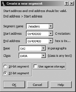
When creating a segment, you may specify any name you wish. Here we choose .headers, because it is unlikely to be used as an actual section name in the file and it adequately describes the section’s content. You may manually enter the section’s start (inclusive) and end (exclusive) addresses, or they will be filled in automatically if you have highlighted the range of addresses that make up the section prior to opening the dialog. The section base value is described in the SDK’s segment.hpp file. In a nutshell, for x86 binaries, IDA computes the virtual address of a byte by shifting the segment base left four bits and adding the offset to the byte (virtual = (base << 4) + offset). A base value of zero should be used when segmentation is not used. The segment class can be used to describe the content of the segment. Several predefined class names such as CODE, DATA, and BSS are recognized. Predefined segment classes are also described in segment.hpp.

An unfortunate side effect of creating a new segment is that any data that had been defined within the bounds of the segment (such as the headers that we previously formatted) will be undefined. After reapplying all of the header structures discussed previously, we return to the header for the .text section to note that the VirtualAddress field (1000h) is an RVA that specifies the memory address at which the section content should be loaded and the SizeOfRawData field (600h) indicates how many bytes of data are present in the file. In other words, this particular section header tells us that the .text section is created by mapping the 600h bytes from file offsets 400h-9FFh to virtual addresses 401000h-4015FFh.

Because our example file was loaded in binary mode, all of the bytes of the .text section are present in the database; we simply need to shift them into their proper locations. Following creation of the .headers section, we might have a display similar to the following at the end of the .headers section:

.headers:004003FF                 db    0
.headers:004003FF _headers        ends
.headers:004003FF
seg001:00400400 ; ===========================================================
seg001:00400400
seg001:00400400 ; Segment type: Pure code
seg001:00400400 seg001          segment byte public 'CODE' use32
seg001:00400400                 assume cs:seg001
seg001:00400400                 ;org 400400h
seg001:00400400                 assume es:_headers, ss:_headers, ds:_headers
seg001:00400400                 db  55h ; U

When the .headers section was created, IDA split the original seg000 to form the .headers section as we specified and a new seg001 to hold the remaining bytes from seg000. The content for the .text section is resident in the database as the first 600h bytes of seg001. We simply need to move the section to the proper location and size the .text section correctly.

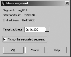
The first step in creating the .text section involves moving seg001 to virtual address 401000h. Using the Edit ▸ Segments ▸ Move Current Segment command, we specify a new start address for seg001, as shown in Figure 18-4.

Figure 18-4. Moving a segment

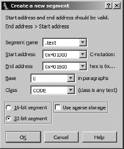
The next step is to carve the .text section from the first 600h bytes of the newly moved seg001 using Edit ▸ Segments ▸ Create Segment. Figure 18-5 shows the parameters, derived from the section header values, used to create the new section.

Keep in mind that the end address is exclusive. Creation of the .text section splits seg001 into the new .text section and all remaining bytes of the original file into a new section named seg002, which immediately follows the .text section.

Figure 18-5. Manual creation of the .text section

Returning to the section headers, we now look at the second section, which appears as follows once it has been structured as an IMAGE_SECTION_HEADER:

.headers:004001A0                 db '.rdata',0,0         ; Name
.headers:004001A0                 dd 60h                  ; VirtualSize
.headers:004001A0                 dd 2000h                ; VirtualAddress
.headers:004001A0                 dd 200h                 ; SizeOfRawData
.headers:004001A0                 dd 0A00h                ; PointerToRawData
.headers:004001A0                 dd 0                    ; PointerToRelocations
.headers:004001A0                 dd 0                    ; PointerToLinenumbers
.headers:004001A0                 dw 0                    ; NumberOfRelocations
.headers:004001A0                 dw 0                    ; NumberOfLinenumbers
.headers:004001A0                 dd 40000040h            ; Characteristics

Using the same data fields we examined for the .text section, we note that this section is named .rdata, occupies 200h bytes in the file beginning at file offset 0A00h, and maps to RVA 2000h (virtual address 402000h). It is important to note at this point that since we moved the .text segment, we can no longer easily map the PointerToRawData field to an offset within the database. Instead, we rely on the fact that the content for the .rdata section immediately follows the content for the .text section. In other words, the .rdata section currently resides in the first 200h bytes of seg002. An alternative approach would be to create the sections in reverse order, beginning with the last section defined in the headers and working our way backwards until we finally create the .text section. This approach leaves sections positioned at their proper file offsets until they are moved to their corresponding virtual addresses.

The creation of the .rdata section proceeds in a manner similar to the creation of the .text section. In the first step, seg002 is moved to 402000h, and in the second step, the actual .rdata section is created to span the address range 402000h-402200h.

The next section defined in this particular binary is called the .bss section. A .bss section is typically generated by compilers as a place to group all statically allocated variables (such as globals) that need to be initialized to zero when the program starts. Static variables with nonzero initial values are typically allocated in a .data (nonconstant) or .rdata (constant) section. The advantage of a .bss section is that it typically requires zero space in the disk image, with space being allocated for the section when the memory image of the executable is created by the operating system loader. In this example, the .bss section is specified as follows:

.headers:004001C8                 db '.bss',0,0,0      ; Name
.headers:004001C8                 dd 40h             ; VirtualSize
.headers:004001C8                 dd 3000h             ; VirtualAddress
.headers:004001C8                 dd 0               ; SizeOfRawData
.headers:004001C8                 dd 0                 ; PointerToRawData
.headers:004001C8                 dd 0                 ; PointerToRelocations
.headers:004001C8                 dd 0                 ; PointerToLinenumbers
.headers:004001C8                 dw 0                 ; NumberOfRelocations
.headers:004001C8                 dw 0                 ; NumberOfLinenumbers
.headers:004001C8                 dd 0C0000080h        ; Characteristics

Here the section header indicates that the size of the section within the file, SizeOfRawData , is zero, while the VirtualSize of the section is 0x40 (64) bytes. In order to create this section in IDA, it is first necessary to create a gap (because we have no file content to populate the section) in the address space beginning at address 0x403000 and then define the .bss section to consume this gap. The easiest way to create this gap is to move the remaining sections of the binary into their proper places. When this task is complete, we might end up with a Segments window listing similar to the following:

Name     Start    End      R W X D L Align Base Type   Class
.headers 00400000 00400400 ? ? ? . . byte  0000 public DATA   ...
.text    00401000 00401600 ? ? ? . . byte  0000 public CODE   ...
.rdata   00402000 00402200 ? ? ? . . byte  0000 public DATA   ...
.bss     00403000 00403040 ? ? ? . . byte  0000 public BSS    ...
.idata   00404000 00404200 ? ? ? . . byte  0000 public IMPORT ...
seg005   00404200 004058DE ? ? ? . L byte  0001 public CODE   ...

The right-hand portion of the listing has been truncated for the sake of brevity. You may notice that the segment end addresses are not adjacent to their subsequent segment start addresses. This is a result of creating the segments using their file sizes rather than taking into account their virtual sizes and any required section alignment. In order to have our segments reflect the true layout of the executable image, we could edit each end address to consume any gaps between segments.

The question marks in the segments list represent unknown values for the permission bits on each section. For PE files, these values are specified via bits in the Characteristics field of each section header. There is no way to specify permissions for manually created sections other than by programmatically using a script or a plug-in. The following IDC statement sets the execute permission on the .text section in the previous listing:

SetSegmentAttr(0x401000, SEGATTR_PERM, 1);

Unfortunately, IDC does not define symbolic constants for each of the allowable permissions. Unix users may find it easy to remember that the section permission bits happen to correspond to the permission bits used in Unix file systems; thus read is 4, write is 2, and execute is 1. You may combine the values using a bitwise OR to set more than one permission in a single operation.

The last step that we will cover in the manual loading process is to finally get the x86 processor module to do some work for us. Once the binary has been properly mapped into various IDA sections, we can return to the program entry point that we found in the headers (RVA 1000h, or virtual address 401000h) and ask IDA to convert the bytes at that location to code. If we wish to have IDA list the address as an entry point in the Exports window, we must programmatically designate it as such. Here is a Python one-liner to do this:

AddEntryPoint(0x401000, 0x401000, 'start', 1);

Called in this manner, IDA will name the entry point 'start', add it as an exported symbol, and create code at the specified address, initiating a recursive descent to disassemble as much related code as possible. Please refer to IDA’s built-in help for more information on the AddEntryPoint function.

When a file is loaded in binary mode, IDA performs no automatic analysis of the file content. Among other things, no attempt is made to identify the compiler used to create the binary, no attempt is made to determine what libraries and functions the binary imports, and no type library or signature information is automatically loaded into the database. In all likelihood, we will need to do a substantial amount of work to produce a disassembly comparable to those we have seen IDA generate automatically. In fact, we have not even touched on other aspects of the PE headers and how we might incorporate such additional information into our manual loading process.

In rounding out our discussion of manual loading, consider that you would need to repeat each of the steps covered in this section every time you open a binary with the same format, one unknown to IDA. Along the way, you might choose to automate some of your actions by writing IDC scripts that perform some of the header parsing and segment creation for you. This is exactly the motivation behind and the purpose for IDA loader modules, which are covered in the next section.