The simplest way to modify a piece of data is to adjust its size. IDA offers a number of data size/type specifiers. The most commonly encountered specifiers are db, dw, and dd, representing 1-, 2-, and 4-byte data, respectively. The first way to change a data item’s size is via the Options ▸ Setup Data Types dialog shown in Figure 7-8.

There are two parts to this dialog. The left side of the dialog contains a column of buttons used to immediately change the data size of the currently selected item. The right side of the dialog contains a column of checkboxes used to configure what IDA terms the data carousel. Note that for each button on the left, there is a corresponding checkbox on the right. The data carousel is a revolving list of datatypes that contains only those types whose checkboxes are selected. Modifying the contents of the data carousel has no immediate impact on the IDA display. Instead, each type on the data carousel is listed on the context-sensitive menu that appears when you right-click a data item. Thus, it is easier to reformat data to a type listed in the data carousel than to a type not listed in the data carousel. Given the datatypes selected in Figure 7-8, right-clicking a data item would offer you the opportunity to reformat that item as byte, word, or double-word data.

Figure 7-8. The datatype setup dialog

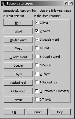
The name for the data carousel derives from the behavior of the associated data formatting hotkey: D. When you press D, the item at the currently selected address is reformatted to the next type in the data carousel list. With the three-item list specified previously, an item currently formatted as db toggles to dw, an item formatted as dw toggles to dd, and an item formatted as dd toggles back to db to complete the circuit around the carousel. Using the data hotkey on a nondata item such as code causes the item to be formatted as the first datatype in the carousel list (db in this case).

Toggling through datatypes causes data items to grow, shrink, or remain the same size. If an item’s size remains the same, then the only observable change is in the way the data is formatted. If you reduce an item’s size, from dd (4 bytes) to db (1 byte) for example, any extra bytes (3 in this case) become undefined. If you increase the size of an item, IDA complains if the bytes following the item are already defined and asks you, in a roundabout way, if you want IDA to undefine the next item in order to expand the current item. The message you encounter in such cases is “Directly convert to data?” This message generally means that IDA will undefine a sufficient number of succeeding items to satisfy your request. For example, when converting byte data (db) to double-word data (dd), 3 additional bytes must be consumed to form the new data item.

Datatypes and sizes can be specified for any location that describes data, including stack variables. To change the size of stack-allocated variables, open the detailed stack frame view by double-clicking the variable you wish to modify; then change the variable’s size as you would any other variable.

IDA recognizes a large number of string formats. By default, IDA searches for and formats C-style null-terminated strings. To force data to be converted to a string, utilize the options on the Edit ▸ Strings menu to select a specific string style. If the bytes beginning at the currently selected address form a string of the selected style, IDA groups those bytes together into a single-string variable. At any time, you can use the A hotkey to format the currently selected location in the default string style.

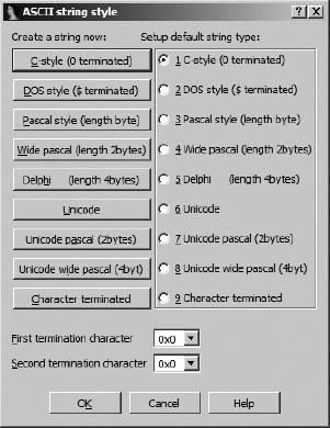
Two dialogs are responsible for the configuration of string data. The first, shown in Figure 7-9, is accessed via Options ▸ ASCII String Style, though ASCII in this case is a bit of a misnomer, as a much wider variety of string styles are understood.

Similar to the datatype configuration dialog, the buttons on the left are used to create a string of the specified style at the currently selected location. A string is created only if the data at the current location conforms to the specified string format. For Character terminated strings, up to two termination characters can be specified toward the bottom of the dialog. The radio buttons on the right of the dialog are used to specify the default string style associated with the use of the strings hotkey (A).

Figure 7-9. String data configuration

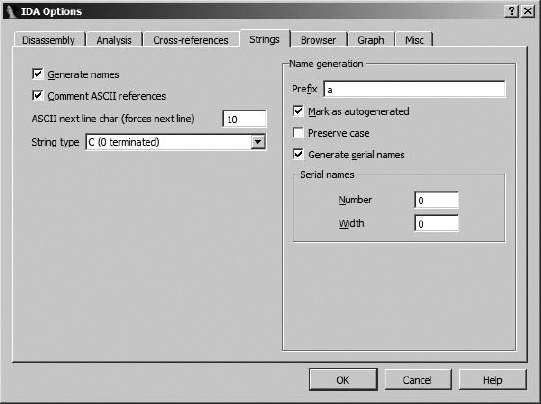
The second dialog used to configure string operations is the Options ▸ General dialog, shown in Figure 7-10, where the Strings tab allows configuration of additional strings-related options. While you can specify the default string type here as well using the available drop-down box, the majority of available options deal with the naming and display of string data, regardless of their type. The Name generation area on the right of the dialog is visible only when the Generate names option is selected. When name generation is turned off, string variables are given dummy names beginning with the asc_ prefix.

Figure 7-10. IDA Strings options

When name generation is enabled, the Name generation options control how IDA generates names for string variables. When Generate serial names is not selected (the default), the specified prefix is combined with characters taken from the string to generate a name that does not exceed the current maximum name length. An example of such a string appears here:

.rdata:00402069 aThisIsACharact db 'This is a Character array',0

Title case is used in the name, and any characters that are not legal to use within names (such as spaces) are omitted when forming the name. The Mark as autogenerated option causes generated names to appear in a different color (dark blue by default) than user-specified names (blue by default). Preserve case forces the name to use characters as they appear within the string rather than converting them to title case. Finally, Generate serial names causes IDA to serialize names by appending numeric suffixes (beginning with Number). The number of digits in generated suffixes is controlled by the Width field. As configured in Figure 7-10, the first three names to be generated would be a000, a001, and a002.

One of the drawbacks to disassembly listings derived from higher-level languages is that they provide very few clues regarding the size of arrays. In a disassembly listing, specifying an array can require a tremendous amount of space if each item in the array is specified on its own disassembly line. The following listing shows data declarations that follow the named variable unk_402060. The fact that only the first item in the listing is referenced by any instructions suggests that it may be the first element in an array. Rather than being referenced directly, additional elements within arrays are often referenced using more complex index computations to offset from the beginning of the array.

.rdata:00402060 unk_402060      db    0    ; DATA XREF: sub_401350+8↑o
.rdata:00402060                            ; sub_401350+18↑o
.rdata:00402061                 db    0
.rdata:00402062                 db    0
.rdata:00402063                 db    0
.rdata:00402064                 db    0
.rdata:00402065                 db    0
.rdata:00402066                 db    0
.rdata:00402067                 db    0
.rdata:00402068                 db    0
.rdata:00402069                 db    0
.rdata:0040206A                 db    0

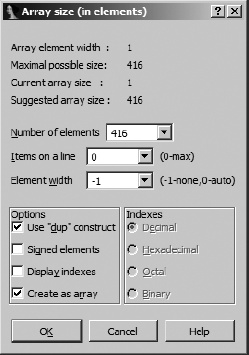
IDA provides facilities for grouping consecutive data definitions together into a single array definition. To create an array, select the first element of the array (we chose unk_402060) and use Edit ▸ Array to launch the array-creation dialog shown in Figure 7-11. If a data item has been defined at a given location, then an Array option will be available when you right-click the item. The type of array to be created is dictated by the datatype associated with the item selected as the first item in the array. In this case we are creating an array of bytes.

Figure 7-11. Array-creation dialog

Following are descriptions of useful fields for array creation:

Accepting the options specified in Figure 7-11 results in the following compact array declaration, which can be read as an array of bytes (db) named byte_402060 consisting of the value 0 repeated 416 (1A0h) times.

.rdata:00402060 byte_402060     db 1A0h dup(0)     ; DATA XREF: sub_401350+8↑o
.rdata:00402060                                    ; sub_401350+18↑o

The net effect is that 416 lines of disassembly have been condensed to a single line (largely due to the use of dup). In the next chapter we will discuss the creation of arrays within stack frames.