Chapter 7. Wrapping Our Heads Around Projections

When you look at a map, you are looking at a two-dimensional representation of a 3D object (the Earth). Because we are, essentially, 'losing' a dimension when we create a map, no map is a perfect representation of the Earth. All maps have some distortion.

The distortion depends on what projection (a method of representing the earth's surface on a two dimensional plane) you use. In this chapter, we'll talk more about what projections are, why they're important, and how we can use them in OpenLayers. We'll also cover some other fundamental geographic principles that will help make it easier to better understand OpenLayers.

In this chapter, we will cover the following topics:

Concept of map projections
Types of projections
Latitude, longitude, and other geographic concepts
The OpenLayers projection class
Transforming coordinates
Projections in context of raster layers
Projections using vector layers

Let's get started!

Map projections

No maps of the earth are truly perfect representations; all maps have some distortion. The reason for this, is because they are attempting to represent a 3D object (an ellipsoid: the Earth) in two dimensions (a plane: the map itself).

A projection is a representation of the entire, or parts of a surface of a 3D sphere (or more precisely, an ellipsoid) on a 2D plane (or other types of geometry).

Why on earth are projections used?

Every map has some sort of projection—it is an inherent attribute of maps. Imagine unpeeling an orange and then flattening the peel out. Some kind of distortion will occur, and if you try to fully fit the peel into a square or rectangle (like a flat, two-dimensional map), you'd have a very hard time.

To get the peel to fit perfectly onto a flat square or rectangle, you can try to stretch out certain parts of the peel or cut some pieces of the peel off and rearrange them. The same sort of idea applies while trying to create a map.

There are literally an infinite amount of possible map projections; an unlimited number of ways to represent a three-dimensional surface in two dimensions, but none of them are totally distortion free.

So, if there are so many different map projections, how do we decide on which one to use? Is there a best one? The answer is no. The 'best' projection to use depends on the context in which you use your map, what you're looking at, and what characteristics you wish to preserve.

Projection characteristics

As a two-dimensional representation is not without distortion, each projection makes a trade off between some characteristics. As we lose a dimension when projecting the earth onto a map, we must make some sort of trade off between the characteristics we want to preserve. There are numerous characteristics, but for now, let's focus on three of them.

Area

Area refers to the size of features on the map. Projections that preserve area are known as equal-area projections (also known as equiareal, equivalent, or homolographic). A projection preserves area if, for example, a meter measured at different places on the map covers the same area. Because area remains the same, angles, scales, and shapes are distorted. This is what an equal area projected map may look like:

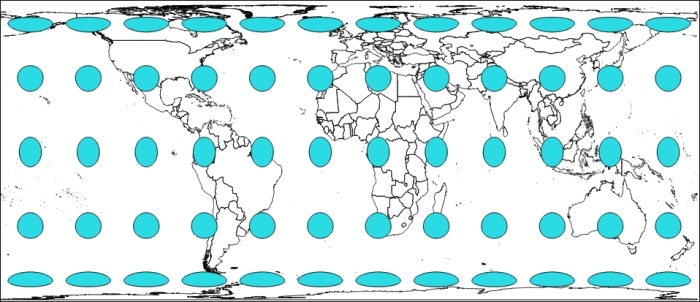
Here, we use Tissot indicatrix with EPSG:3410 NSIDC EASE-Grid Global, where the EPSG code helps define all existing projections. We will cover EPSG in detail, later in this chapter.

Without going into technical details, Tissot indicatrix is a way to display map projections deformation visually. In a perfect projection, we will keep area, distance, and shape, with circles with equal area and equal distance.

As you see, with this equal-area projection, we have circle and ellipse shapes but areas remain the same.

Scale

Scale is the ratio of the map's distance to the actual distance (for example, one centimeter on the map may be equal to one hundred actual meters). All map projections show scale incorrectly at some areas throughout the map; no map can show the same scale throughout the map. There are parts of the map, however, where scale remains correct—the placement of these locations mitigates scale errors elsewhere. The deformation of scale also depends on the area being mapped. Projections are referred to as equidistant if they contain true scale between a point and every other point on the map.

An example to illustrate can be the EPSG:32662 projection known as Plate Carree.

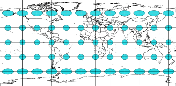
Here, we keep the distance between the center of the ellipse/circle. We overlay on top of the image of a grid so that you can better evaluate distance.

Shape

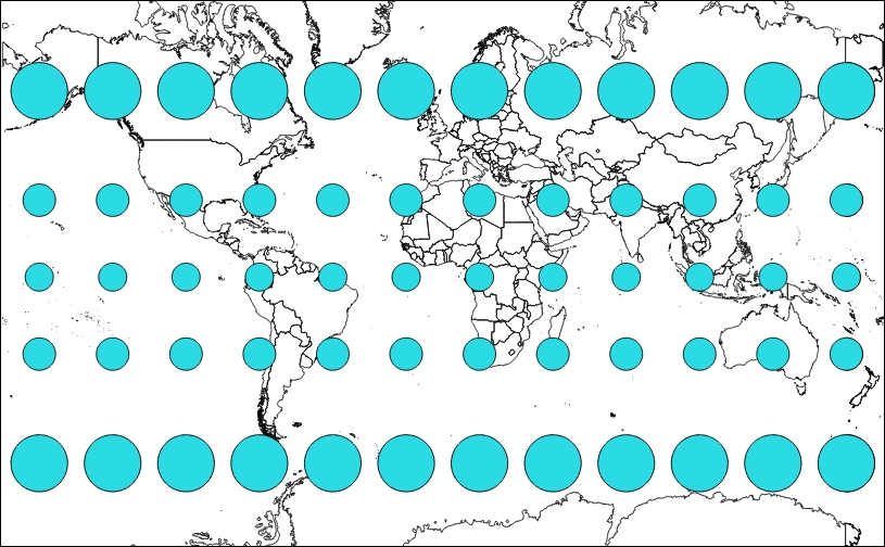
Maps that preserve shape are known as conformal or orthomorphic. Shape means that relative angles to all points on a map are correct. Most maps that show the entire earth are conformal, such as the Mercator projection (used by Google Earth and other common web maps). Depending on the specific projection, areas throughout the map are generally distorted but may be correct in certain places. Also, a map that is conformal cannot be equal-area.

To illustrate shape preservations, let's see the following example using EPSG code 3395 (WGS 84 - World Mercator), where all circles stay circles wherever they are:

Other characteristics

Projections have numerous other characteristics, such as bearing, distance, and direction. The key concept to take away here is that all projections preserve some characteristics at the expense of others. For instance, a map that preserves shape cannot completely preserve area.

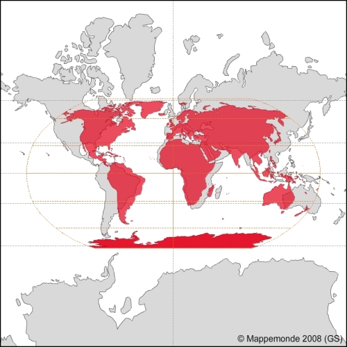
There is no perfect map projection. The usefulness of a projection depends on the context the map is being used in. A particular projection may excel at a certain task, for example, navigation, but can be a poor choice for other purposes. For example, when we do thematic mapping and respect representations rules, colors are related to areas of countries. When we look at a world thematic map with a wrong projection, our eyes see a country bigger than the others, whereas because of projections, this country can, in reality, have a calculated area identical to countries represented with a smaller size.

The following figure overlays an area preserving projection (Robinson) on top of a Spherical Mercator to show the difference and why it matters:

Have a go hero – projections' effects on scale

One of the simple ways to convince you that each projection has a reason to exist is to visit the OpenLayers 3 website examples.

We will compare the scale line example, http://openlayers.org/en/v3.0.0/examples/scale-, with the tiled WMS with the custom projection example, http://openlayers.org/en/v3.0.0/examples/wms-custom-proj.html.

Your instructions until now are:

To not look at the code but only the behavior of the scale line in the bottom-left corner of the map.
In both cases, to zoom in and at the same zoom level, pan up and down looking at the scale line.
How the scale line behaves.
How do you explain it?

Types of projections

Projections are projected onto a geometric surface, three of the most common ones being a plane, cone, or cylinder.

Imagine a cylinder being wrapped around the earth, with the center of the cylinder's circumference touching the equator. Now, the earth is projected onto the surface of this cylinder, and if you cut the cylinder from top to bottom vertically and unwrap it and lay it flat, you'd have a regular cylindrical projection:

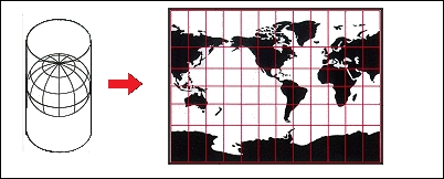
The Mercator projection is just one of these types of projections. If you've never worked with projections before, there is a good chance that most of the maps you've seen were in this projection.

Because of its nature, there is heavy distortion near the ends of the poles. Looking at the previous screenshot, you can see that the cells get progressively larger, the closer you get to the North and South poles. For example, Greenland looks larger than South America, but in reality, it is about the size of Mexico. For illustrating this problem visually, you can compare countries overlapping with http://overlapmaps.com. If area distortion is important in your map, you might consider using an equal area projection, as we mentioned earlier.

Note

More information about projections can be found at the USGS (US Geological Survey) website at http://pubs.er.usgs.gov/publication/pp1395, where you can download the reference book Map Projections: A Working Manual (U.S. Geological Survey Professional Paper 1395), John P. Snyder, 1987, 397 pages.

EPSG codes

As we mentioned, there are literally an infinite number of possible projections. So, it makes sense that there should be some universally agreed upon classification system that keeps track of projection information. There are many different classification systems, but OpenLayers uses EPSG codes. EPSG refers to the European Petroleum Survey Group, a scientific organization involved in oil exploration, which in 2005 was taken over by the OGP (International Association of Oil and Gas Producers).

For the purpose of OpenLayers, EPSG codes are referred to as EPSG:4326.

The numbers (4326, in this case) after EPSG: refer to the projection identification number. It uses the familiar longitude/latitude coordinate system, with coordinates that range from -180° to 180° (longitude) and -90° to 90° (latitude).

Previous Chapter

Summary

Next Chapter

Time for action – using different projection codes