In this section, we are going to implement the Fourier transformation and its backward transformation and then play around with it to transform some signals:
- First, we include all the headers and declare that we use the std namespace:
      #include <iostream>
      #include <complex>
      #include <vector>
      #include <algorithm>
      #include <iterator>
      #include <numeric>
      #include <valarray>
      #include <cmath>

      using namespace std;
- A data point of a signal is a complex number and shall be represented by std::complex, specialized on the double type. This way, the type alias cmplx stands for two coupled double values, which represent the real and the imaginary parts of a complex number. A whole signal is a vector of such items, which we alias to the csignal type:
      using cmplx   = complex<double>;
      using csignal = vector<cmplx>;
- In order to iterate over an up-counting numeric sequence, we take the numeric iterator from the numeric iterator recipe. The variables k and j in the formula shall iterate over such sequences:
      class num_iterator {
          size_t i;
      public:
          explicit num_iterator(size_t position) : i{position} {}

          size_t operator*() const { return i; }

          num_iterator& operator++() {
              ++i;
              return *this;
          }

          bool operator!=(const num_iterator &other) const {
              return i != other.i;
          }
      };
- The Fourier transformation function shall just take a signal and return a new signal. The returned signal represents the Fourier transformation of the input signal. As the back transformation from a Fourier transformed signal back to the original signal is very similar, we provide an optional bool parameter, which chooses the transformation direction. Note that bool parameters are generally bad practice, especially if we use multiple bool parameters in a function signature. Here we just have one for brevity.
The first thing we do is allocate a new signal vector with the size of the initial signal:
      csignal fourier_transform(const csignal &s, bool back = false)
      {
          csignal t (s.size());
- There are two factors in the formula, which always look the same. Let's pack them in their own variables:
          const double pol {2.0 * M_PI * (back ? -1.0 : 1.0)};
          const double div {back ? 1.0 : double(s.size())};
- The std::accumulate algorithm is a fitting choice for executing formulas that sum up items. We are going to use accumulate on a range of up-counting numeric values. From these values, we can form the individual summands of each step. The std::accumulate algorithm calls a binary function on every step. The first parameter of this function is the current value of the part of sum that was already calculated in the previous steps, and its second parameter is the next value from the range. We look up the value of signal s at the current position and multiply it with the complex factor, pol. Then, we return the new partly sum. The binary function is wrapped into another lambda expression because we are going to use different values of j for every accumulate call. Because this is a two-dimensional loop algorithm, the inner lambda is for the inner loop and the outer lambda is for the outer loop:
          auto sum_up ([=, &s] (size_t j) {
              return [=, &s] (cmplx c, size_t k) {
                  return c + s[k] *
                      polar(1.0, pol * k * j / double(s.size()));
              };
          });
- The inner loop part of the Fourier transform is now executed by std::accumulate. For every j position of the algorithm, we calculate the sum of all the summands for positions i = 0...N. This idea is wrapped into a lambda expression, which we will execute for every data point in the resulting Fourier transformation vector:
          auto to_ft ([=, &s](size_t j){
              return accumulate(num_iterator{0},
                                num_iterator{s.size()},
                                cmplx{},
                                sum_up(j))
                  / div;
          });
- None of the Fourier code has been executed until this point. We only prepared a lot of functional code, which we'll put to action now. An std::transform call will generate values j = 0...N, which is our outer loop. The transformed values all go to the vector t, which we then return to the caller:
          transform(num_iterator{0}, num_iterator{s.size()},
                    begin(t), to_ft);

          return t;
      }
- We are going to implement some functions that help us set up function objects for signal generation. The first one is a cosine signal generator. It returns a lambda expression that can generate a cosine signal with the period length that was provided as a parameter. The signal itself can be of arbitrary length, but it has a fixed period length. A period length of N means that the signal will repeat itself after N steps. The lambda expression does not accept any parameters. We can call it repeatedly, and for every call, it returns us the signal data point of the next point in time:
      static auto gen_cosine (size_t period_len){
          return [period_len, n{0}] () mutable {
              return cos(double(n++) * 2.0 * M_PI / period_len);
          };
      }
- Another signal we are going to generate is the square wave. It oscillates between the values -1 and +1 and has no other values than those. The formula looks complicated, but it simply transforms the linearly up-counting value n to +1 and -1, with an oscillating period length of period_len.
Note that we initialize n to a different value from 0 this time. This way, our square wave starts at the phase where its output values begin at +1:
      static auto gen_square_wave (size_t period_len)
      {
          return [period_len, n{period_len*7/4}] () mutable {
              return ((n++ * 2 / period_len) % 2) * 2 - 1.0;
          };
      }
- Generating an actual signal from such generators can be achieved by allocating a new vector and filling it with the values generated from repeating signal generator function calls. The std::generate does this job. It accepts a begin/end iterator pair and a generator function. For every valid iterator position, it does *it = gen(). By wrapping this code into a function, we can easily generate signal vectors:
      template <typename F>
      static csignal signal_from_generator(size_t len, F gen)
      {
          csignal r (len);
          generate(begin(r), end(r), gen);
          return r;
      }
- In the end, we need to print the resulting signals. We can simply print a signal by copying its values into an output stream iterator, but we need to transform the data first because the data points of our signals are complex value pairs. At this point, we are only interested in the real value part of every data point; hence, we throw it through an std::transform call, which extracts only this part:
      static void print_signal (const csignal &s)
      {
          auto real_val ([](cmplx c) { return c.real(); });
          transform(begin(s), end(s),
                    ostream_iterator<double>{cout, " "}, real_val);
          cout << 'n';
      }
- The Fourier formula is now implemented, but we have no signals to transform yet. That is what we do in the main function. Let's first define a standard signal length to which all the signals comply.
      int main()
      {
          const size_t sig_len {100};
- Let's now generate signals, transform them, and print them, which happens in the next three steps. The first step is to generate a cosine signal and a square wave signal. Both have the same total signal length and period length:
          auto cosine      (signal_from_generator(sig_len,
                 gen_cosine(     sig_len / 2)));
          auto square_wave (signal_from_generator(sig_len,
                 gen_square_wave(sig_len / 2)));
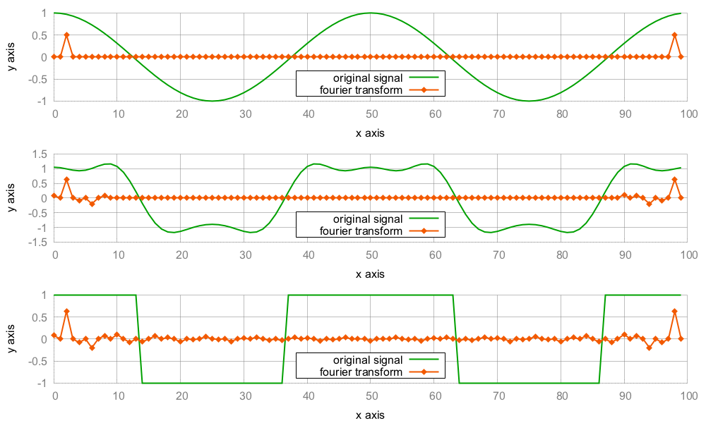
- We have a cosine function and a square wave signal now. In order to generate a third one in the middle between them, we take the square wave signal and calculate its Fourier transform (saved in the trans_sqw vector). The Fourier transform of a square wave has a specific form, and we are going to manipulate it a bit. All items from index 10 till (signal_length - 10) are set to 0.0. The rest remains untouched. Transforming this altered Fourier transformation back to the signal time representation will give us a different signal. We will see how that looks in the end:
          auto trans_sqw (fourier_transform(square_wave));

          fill (next(begin(trans_sqw), 10), prev(end(trans_sqw), 10), 0);
          auto mid (fourier_transform(trans_sqw, true));
- Now we have three signals: cosine, mid, and square_wave. For every signal, we print the signal itself and its Fourier transformation. The output of the whole program will consist of six very long lines of printed double value lists:
          print_signal(cosine);
          print_signal(fourier_transform(cosine));

          print_signal(mid);
          print_signal(trans_sqw);

          print_signal(square_wave);
          print_signal(fourier_transform(square_wave));
      }
- Compiling and running the program leads to the terminal getting filled with lots of numeric values. If we plot the output, we get the following image: