sudo apt install ruby-dev
Expert C++ Programming
Leveraging the power of modern C++ to build scalable modular applications
A learning path in three sections

BIRMINGHAM - MUMBAI

Copyright © 2018 Packt Publishing
All rights reserved. No part of this learning path may be reproduced, stored in a retrieval system, or transmitted in any form or by any means, without the prior written permission of the publisher, except in the case of brief quotations embedded in critical articles or reviews.
Every effort has been made in the preparation of this learning path to ensure the accuracy of the information presented. However, the information contained in this learning path is sold without warranty, either express or implied. Neither the authors, nor Packt Publishing or its dealers and distributors, will be held liable for any damages caused or alleged to have been caused directly or indirectly by this learning path.
Packt Publishing has endeavored to provide trademark information about all of the companies and products mentioned in this learning path by the appropriate use of capitals. However, Packt Publishing cannot guarantee the accuracy of this information.
Authors: Jeganathan Swaminathan, Maya Posch, Jacek Galowicz
Reviewer: Brandon James, Louis E. Mauget, Arne Mertz
Content Development Editor: Priyanka Sawant
Graphics: Jisha Chirayal
Production Coordinator: Nilesh Mohite
Published on: April 2018
Production reference: 1060418
Published by Packt Publishing Ltd.
Livery Place
35 Livery Street
Birmingham
B3 2PB, UK.
ISBN 978-1-78883-139-0

Mapt is an online digital library that gives you full access to over 5,000 books and videos, as well as industry leading tools to help you plan your personal development and advance your career. For more information, please visit our website.
Spend less time learning and more time coding with practical eBooks and Videos from over 4,000 industry professionals
Improve your learning with Skill Plans built especially for you
Get a free eBook or video every month
Mapt is fully searchable
Copy and paste, print, and bookmark content
Did you know that Packt offers eBook versions of every book published, with PDF and ePub files available? You can upgrade to the eBook version at www.PacktPub.com and as a print book customer, you are entitled to a discount on the eBook copy. Get in touch with us at service@packtpub.com for more details.
At www.PacktPub.com, you can also read a collection of free technical articles, sign up for a range of free newsletters, and receive exclusive discounts and offers on Packt books and eBooks.
C++ has come a long way and has now been adopted in several contexts. Its key strengths are its software infrastructure and resource-constrained applications. The C++ 17 release will change the way developers write code, and this course will help you master your developing skills with C++. With real-world, practical examples explaining each concept, the course is divided into three modules where will begin by introducing you to the latest features in C++ 17. It encourages clean code practices in C++ in general and demonstrates the GUI app-development options in C++. You’ll get tips on avoiding memory leaks using smart-pointers.
In the next module, you’ll see how multi-threaded programming can help you achieve concurrency in your applications. We start with a brief introduction to the fundamentals of multithreading and concurrency concepts. We then take an in-depth look at how these concepts work at the hardware-level as well as how both operating systems and frameworks use these low-level functions.
You will learn about the native multithreading and concurrency support available in C++ since the 2011 revision, synchronization and communication between threads, debugging concurrent C++ applications, and the best programming practices in C++.
Moving on, you’ll get an in-depth understanding of the C++ Standard Template Library. Where we show implementation-specific, problem-solution approach that will help you quickly overcome hurdles. You will learn the core STL concepts, such as containers, algorithms, utility classes, lambda expressions, iterators, and more while working on practical real-world recipes. These recipes will help you get the most from the STL and show you how to program in a better way.
This course is for intermediate to advanced level C++ developers who want to get the most out of C++ to build concurrent and scalable application.
Section 1, Mastering C++ Programming, introducing you to the latest features in C++ 17 and STL. It encourages clean code practices in C++ in general and demonstrates the GUI app-development options in C++. You’ll get tips on avoiding memory leaks using smart-pointers.
Section 2, Mastering C++ Multithreading, you’ll see how multi-threaded programming can help you achieve concurrency in your applications. We start with a brief introduction to the fundamentals of multithreading and concurrency concepts. We then take an in-depth look at how these concepts work at the hardware-level as well as how both operating systems and frameworks use these low-level functions. You will learn about the native multithreading and concurrency support available in C++ since the 2011 revision, synchronization and communication between threads, debugging concurrent C++ applications, and the best programming practices in C++.
Section 3, C++17 STL Cookbook, you’ll get an in-depth understanding of the C++ Standard Template Library; we show implementation-specific, problem-solution approaches that will help you quickly overcome hurdles. You will learn the core STL concepts, such as containers, algorithms, utility classes, lambda expressions, iterators, and more while working on practical real-world recipes. These recipes will help you get the most from the STL and show you how to program in a better way.
A strong understanding of C++ language is highly recommended as the book is for the experienced developers. You will need any OS (Windows, Linux, or macOS) and any C++ compiler installed on your systems in order to get started.
You can download the example code files for this learning path from your account at www.packtpub.com. If you purchased this learning path elsewhere, you can visit www.packtpub.com/support and register to have the files emailed directly to you.
You can download the code files by following these steps:
Once the file is downloaded, please make sure that you unzip or extract the folder using the latest version of:
The code bundle for the learning path is also hosted on GitHub at https://github.com/PacktPublishing/Expert-Cpp-Programming. We also have other code bundles from our rich catalog of books and videos available at https://github.com/PacktPublishing/. Check them out!
There are a number of text conventions used throughout this book.
CodeInText: Indicates code words in text, database table names, folder names, filenames, file extensions, pathnames, dummy URLs, user input, and Twitter handles. Here is an example: "Mount the downloaded WebStorm-10*.dmg disk image file as another disk in your system."
A block of code is set as follows:
html, body, #map {
 height: 100%;
 margin: 0;
 padding: 0
}
When we wish to draw your attention to a particular part of a code block, the relevant lines or items are set in bold:
[default]
exten => s,1,Dial(Zap/1|30)
exten => s,2,Voicemail(u100)
exten => s,102,Voicemail(b100)
exten => i,1,Voicemail(s0)
Any command-line input or output is written as follows:
$ mkdir css
$ cd css
Bold: Indicates a new term, an important word, or words that you see onscreen. For example, words in menus or dialog boxes appear in the text like this. Here is an example: "Select System info from the Administration panel."
Feedback from our readers is always welcome.
General feedback: Email feedback@packtpub.com and mention the learning path title in the subject of your message. If you have questions about any aspect of this learning path, please email us at questions@packtpub.com.
Errata: Although we have taken every care to ensure the accuracy of our content, mistakes do happen. If you have found a mistake in this learning path, we would be grateful if you would report this to us. Please visit www.packtpub.com/submit-errata, selecting your learning path, clicking on the Errata Submission Form link, and entering the details.
Piracy: If you come across any illegal copies of our works in any form on the Internet, we would be grateful if you would provide us with the location address or website name. Please contact us at copyright@packtpub.com with a link to the material.
If you are interested in becoming an author: If there is a topic that you have expertise in and you are interested in either writing or contributing to a book, please visit authors.packtpub.com.
Please leave a review. Once you have read and used this learning path, why not leave a review on the site that you purchased it from? Potential readers can then see and use your unbiased opinion to make purchase decisions, we at Packt can understand what you think about our products, and our authors can see your feedback on their book. Thank you!
For more information about Packt, please visit packtpub.com.
As you know, the C++ language is the brain child of Bjarne Stroustrup, who developed C++ in 1979. The C++ programming language is standardized by International Organization for Standardization (ISO). The initial standardization was published in 1998, commonly referred to as C++98, and the next standardization C++03 was published in 2003, which was primarily a bug fix release with just one language feature for value initialization. In August 2011, the C++11 standard was published with several additions to the core language, including several significant interesting changes to the Standard Template Library (STL); C++11 basically replaced the C++03 standard. C++14 was published in December, 2014 with some new features, and later, the C++17 standard was published on July 31, 2017. At the time of writing this book, C++17 is the latest revision of the ISO/IEC standard for the C++ programming language.
This chapter requires a compiler that supports C++17 features: gcc version 7 or later. As gcc version 7 is the latest version at the time of writing this book, I'll be using gcc version 7.1.0 in this chapter.
This chapter will cover the following topics:
Let's look into the STL topics one by one in the following sections.
The C++ Standard Template Library (STL) offers ready-made generic containers, algorithms that can be applied to the containers, and iterators to navigate the containers. The STL is implemented with C++ templates, and templates allow generic programming in C++.
The STL encourages a C++ developer to focus on the task at hand by freeing up the developer from writing low-level data structures and algorithms. The STL is a time-tested library that allows rapid application development.
The STL is an interesting piece of work and architecture. Its secret formula is compile-time polymorphism. To get better performance, the STL avoids dynamic polymorphism, saying goodbye to virtual functions. Broadly, the STL has the following four components:
The STL architecture stitches all the aforementioned four components together. It has many commonly used algorithms with performance guarantees. The interesting part about STL algorithms is that they work seamlessly without any knowledge about the containers that hold the data. This is made possible due to the iterators that offer high-level traversal APIs, which completely abstracts the underlying data structure used within a container. The STL makes use of operator overloading quite extensively. Let's understand the major components of STL one by one to get a good grasp of the STL conceptually.
The STL algorithms are powered by C++ templates; hence, the same algorithm works irrespective of what data type it deals with or independently of how the data is organized by a container. Interestingly, the STL algorithms are generic enough to support built-in and user-defined data types using templates. As a matter of fact, the algorithms interact with the containers via iterators. Hence, what matters to the algorithms is the iterator supported by the container. Having said that, the performance of an algorithm depends on the underlying data structure used within a container. Hence, certain algorithms work only on selective containers, as each algorithm supported by the STL expects a certain type of iterator.
An iterator is a design pattern, but interestingly, the STL work started much before
Gang of Four published their design patterns-related work to the software community. Iterators themselves are objects that allow traversing the containers to access, modify, and manipulate the data stored in the containers. Iterators do this so magically that we don't realize or need to know where and how the data is stored and retrieved.
The following image visually represents an iterator:
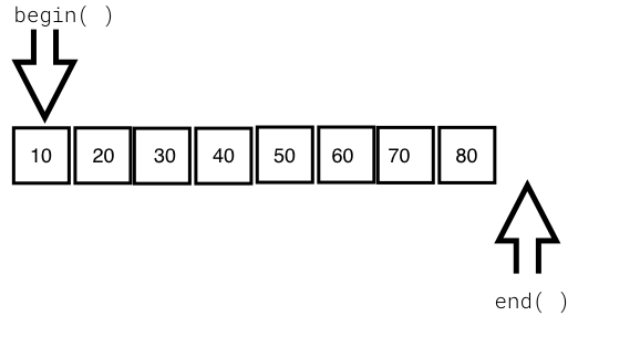
From the preceding image, you can understand that every iterator supports the begin() API, which returns the first element position, and the end() API returns one position past the last element in the container.
The STL broadly supports the following five types of iterators:
The container implements the iterator to let us easily retrieve and manipulate the data, without delving much into the technical details of a container.
The following table explains each of the five iterators:
|
The type of iterator |
Description |
|
Input iterator |
|
|
Output iterator |
|
|
Forward iterator |
|
|
Bidirectional iterator |
|
|
Random-access iterator |
|
STL containers are objects that typically grow and shrink dynamically. Containers use complex data structures to store the data under the hood and offer high-level functions to access the data without us delving into the complex internal implementation details of the data structure. STL containers are highly efficient and time-tested.
Every container uses different types of data structures to store, organize, and manipulate data in an efficient way. Though many containers may seem similar, they behave differently under the hood. Hence, the wrong choice of containers leads to application performance issues and unnecessary complexities.
Containers come in the following flavors:
The objects stored in the containers are copied or moved, and not referenced. We will explore every type of container in the upcoming sections with simple yet interesting examples.
Functors are objects that behave like regular functions. The beauty is that functors can be substituted in the place of function pointers. Functors are handy objects that let you extend or complement the behavior of an STL function without compromising the object-oriented coding principles.
Functors are easy to implement; all you need to do is overload the function operator. Functors are also referred to as functionoids.
The following code will demonstrate the way a simple functor can be implemented:
#include <iostream>
#include <vector>
#include <iterator>
#include <algorithm>
using namespace std;

template <typename T>
class Printer {
public:
  void operator() ( const T& element ) {
    cout << element << "t";
  }
};

int main () {
  vector<int> v = { 10, 20, 30, 40, 50 };

  cout << "nPrint the vector entries using Functor" << endl;

  for_each ( v.begin(), v.end(), Printer<int>() );

  cout << endl;

  return 0;
}
Let's quickly compile the program using the following command:
g++ main.cpp -std=c++17
./a.out
Let's check the output of the program:
Print the vector entries using Functor
10  20  30  40  50
We hope you realize how easy and cool a functor is.
The STL supports quite an interesting variety of sequence containers. Sequence containers store homogeneous data types in a linear fashion, which can be accessed sequentially. The STL supports the following sequence containers:
As the objects stored in an STL container are nothing but copies of the values, the STL expects certain basic requirements from the user-defined data types in order to hold those objects inside a container. Every object stored in an STL container must provide the following as a minimum requirement:
Let's explore the sequence containers one by one in the following subsections.
The STL array container is a fixed-size sequence container, just like a C/C++ built-in array, except that the STL array is size-aware and a bit smarter than the built-in C/C++ array. Let's understand an STL array with an example:
#include <iostream>
#include <array>
using namespace std;
int main () {
  array<int,5> a = { 1, 5, 2, 4, 3 };

  cout << "nSize of array is " << a.size() << endl;

  auto pos = a.begin();

  cout << endl;
  while ( pos != a.end() )
    cout << *pos++ << "t";
  cout << endl;

  return 0;
}
The preceding code can be compiled and the output can be viewed with the following commands:
g++ main.cpp -std=c++17
./a.out
The output of the program is as follows:
Size of array is 5
1     5     2     4     3
The following line declares an array of a fixed size (5) and initializes the array with five elements:
array<int,5> a = { 1, 5, 2, 4, 3 };
The size mentioned can't be changed once declared, just like a C/C++ built-in array. The array::size() method returns the size of the array, irrespective of how many integers are initialized in the initializer list. The auto pos = a.begin() method declares an iterator of array<int,5> and assigns the starting position of the array. The array::end() method points to one position after the last element in the array. The iterator behaves like or mimics a C++ pointer, and dereferencing the iterator returns the value pointed by the iterator. The iterator position can be moved forward and backwards with ++pos and --pos, respectively.
The following table shows some commonly used array APIs:
|
API |
Description |
|
at( int index ) |
This returns the value stored at the position referred to by the index. The index is a zero-based index. This API will throw an std::out_of_range exception if the index is outside the index range of the array. |
|
operator [ int index ] |
This is an unsafe method, as it won't throw any exception if the index falls outside the valid range of the array. This tends to be slightly faster than at, as this API doesn't perform bounds checking. |
|
front() |
This returns the first element in the array. |
|
back() |
This returns the last element in the array. |
|
begin() |
This returns the position of the first element in the array |
|
end() |
This returns one position past the last element in the array |
|
rbegin() |
This returns the reverse beginning position, that is, it returns the position of the last element in the array |
|
rend() |
This returns the reverse end position, that is, it returns one position before the first element in the array |
|
size() |
This returns the size of the array |
The array container supports random access; hence, given an index, the array container can fetch a value with a runtime complexity of O(1) or constant time.
The array container elements can be accessed in a reverse fashion using the reverse iterator:
#include <iostream>
#include <array>
using namespace std;

int main () {

    array<int, 6> a;
    int size = a.size();
    for (int index=0; index < size; ++index)
         a[index] = (index+1) * 100;

    cout << "nPrint values in original order ..." << endl;

    auto pos = a.begin();
    while ( pos != a.end() )
        cout << *pos++ << "t";
    cout << endl;

    cout << "nPrint values in reverse order ..." << endl;

    auto rpos = a.rbegin();
    while ( rpos != a.rend() )
    cout << *rpos++ << "t";
    cout << endl;

    return 0;
}
We will use the following command to get the output:
./a.out
The output is as follows:
Print values in original order ...
100   200   300   400   500   600

Print values in reverse order ...
600   500   400   300   200   100
Vector is a quite useful sequence container, and it works exactly as an array, except that the vector can grow and shrink at runtime while an array is of a fixed size. However, the data structure used under the hood in an array and vector is a plain simple built-in C/C++ style array.
Let's look at the following example to understand vectors better:
#include <iostream>
#include <vector>
#include <algorithm>
using namespace std;

int main () {
  vector<int> v = { 1, 5, 2, 4, 3 };

  cout << "nSize of vector is " << v.size() << endl;

  auto pos = v.begin();

  cout << "nPrint vector elements before sorting" << endl;
  while ( pos != v.end() )
    cout << *pos++ << "t";
  cout << endl;

  sort( v.begin(), v.end() );

  pos = v.begin();

  cout << "nPrint vector elements after sorting" << endl;

  while ( pos != v.end() )
    cout << *pos++ << "t";
  cout << endl;

  return 0;
}
The preceding code can be compiled and the output can be viewed with the following commands:
g++ main.cpp -std=c++17
./a.out
The output of the program is as follows:
Size of vector is 5

Print vector elements before sorting
1     5     2     4     3

Print vector elements after sorting
1     2     3     4     5
The following line declares a vector and initializes the vector with five elements:
vector<int> v = { 1, 5, 2, 4, 3 };
However, a vector also allows appending values to the end of the vector by using the vector::push_back<data_type>( value ) API. The sort() algorithm takes two random access iterators that represent a range of data that must be sorted. As the vector internally uses a built-in C/C++ array, just like the STL array container, a vector also supports random access iterators; hence the sort() function is a highly efficient algorithm whose runtime complexity is logarithmic, that is, O(N log2 (N)).
The following table shows some commonly used vector APIs:
|
API |
Description |
|
at ( int index ) |
This returns the value stored at the indexed position. It throws the std::out_of_range exception if the index is invalid. |
|
operator [ int index ] |
This returns the value stored at the indexed position. It is faster than at( int index ), since no bounds checking is performed by this function. |
|
front() |
This returns the first value stored in the vector. |
|
back() |
This returns the last value stored in the vector. |
|
empty() |
This returns true if the vector is empty, and false otherwise. |
|
size() |
This returns the number of values stored in the vector. |
|
reserve( int size ) |
This reserves the initial size of the vector. When the vector size has reached its capacity, an attempt to insert new values requires vector resizing. This makes the insertion consume O(N) runtime complexity. The reserve() method is a workaround for the issue described. |
|
capacity() |
This returns the total capacity of the vector, while the size is the actual value stored in the vector. |
|
clear() |
This clears all the values. |
|
push_back<data_type>( value ) |
This adds a new value at the end of the vector. |
It would be really fun and convenient to read and print to/from the vector using istream_iterator and ostream_iterator. The following code demonstrates the use of a vector:
#include <iostream>
#include <vector>
#include <algorithm>
#include <iterator>
using namespace std;

int main () {
    vector<int> v;

    cout << "nType empty string to end the input once you are done feeding the vector" << endl;
    cout << "nEnter some numbers to feed the vector ..." << endl;


    istream_iterator<int> start_input(cin);
    istream_iterator<int> end_input;

    copy ( start_input, end_input, back_inserter( v ) );


    cout << "nPrint the vector ..." << endl;
    copy ( v.begin(), v.end(), ostream_iterator<int>(cout, "t") );
    cout << endl;


    return 0;
}
Basically, the copy algorithm accepts a range of iterators, where the first two arguments represent the source and the third argument represents the destination, which happens to be the vector:
istream_iterator<int> start_input(cin);
istream_iterator<int> end_input;

copy ( start_input, end_input, back_inserter( v ) );
The start_input iterator instance defines an istream_iterator iterator that receives input from istream and cin, and the end_input iterator instance defines an end-of-file delimiter, which is an empty string by default (""). Hence, the input can be terminated by typing "" in the command-line input terminal.
Similarly, let's understand the following code snippet:
cout << "nPrint the vector ..." << endl;
copy ( v.begin(), v.end(), ostream_iterator<int>(cout, "t") );
cout << endl;
The copy algorithm is used to copy the values from a vector, one element at a time, to ostream, separating the output with a tab character (t).
Every STL container has its own advantages and disadvantages. There is no single STL container that works better in all the scenarios. A vector internally uses an array data structure, and arrays are fixed in size in C/C++. Hence, when you attempt to add new values to the vector at the time the vector size has already reached its maximum capacity, then the vector will allocate new consecutive locations that can accommodate the old values and the new value in a contiguous location. It then starts copying the old values into the new locations. Once all the data elements are copied, the vector will invalidate the old location.
Whenever this happens, the vector insertion will take O(N) runtime complexity. As the size of the vector grows over time, on demand, the O(N) runtime complexity will show up a pretty bad performance. If you know the maximum size required, you could reserve so much initial size upfront in order to overcome this issue. However, not in all scenarios do you need to use a vector. Of course, a vector supports dynamic size and random access, which has performance benefits in some scenarios, but it is possible that the feature you are working on may not really need random access, in which case a list, deque, or some other container may work better for you.
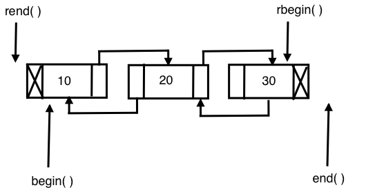
The list STL container makes use of a doubly linked list data structure internally. Hence, a list supports only sequential access, and searching a random value in a list in the worst case may take O(N) runtime complexity. However, if you know for sure that you only need sequential access, the list does offer its own benefits. The list STL container lets you insert data elements at the end, in the front, or in the middle with a constant time complexity, that is, O(1) runtime complexity in the best, average, and worst case scenarios.
The following image demonstrates the internal data structure used by the list STL:
Let's write a simple program to get first-hand experience of using the list STL:
#include <iostream>
#include <list>
#include <iterator>
#include <algorithm>
using namespace std;

int main () {

  list<int> l;

  for (int count=0; count<5; ++count)
    l.push_back( (count+1) * 100 );

  auto pos = l.begin();

  cout << "nPrint the list ..." << endl;
  while ( pos != l.end() )
    cout << *pos++ << "-->";
  cout << " X" << endl;

  return 0;
}
I'm sure that by now you have got a taste of the C++ STL, its elegance, and its power. Isn't it cool to observe that the syntax remains the same for all the STL containers? You may have observed that the syntax remains the same no matter whether you are using an array, a vector, or a list. Trust me, you will get the same impression when you explore the other STL containers as well.
Having said that, the previous code is self-explanatory, as we did pretty much the same with the other containers.
Let's try to sort the list, as shown in the following code:
#include <iostream>
#include <list>
#include <iterator>
#include <algorithm>
using namespace std;

int main () {

    list<int> l = { 100, 20, 80, 50, 60, 5 };

    auto pos = l.begin();

    cout << "nPrint the list before sorting ..." << endl;
    copy ( l.begin(), l.end(), ostream_iterator<int>( cout, "-->" ));
    cout << "X" << endl;

    l.sort();

    cout << "nPrint the list after sorting ..." << endl;
    copy ( l.begin(), l.end(), ostream_iterator<int>( cout, "-->" ));
    cout << "X" << endl;

    return 0;
}
Did you notice the sort() method? Yes, the list container has its own sorting algorithms. The reason for a list container to support its own version of a sorting algorithm is that the generic sort() algorithm expects a random access iterator, whereas a list container doesn't support random access. In such cases, the respective container will offer its own efficient algorithms to overcome the shortcoming.
Interestingly, the runtime complexity of the sort algorithm supported by a list is O (N log2 N).
The following table shows the most commonly used APIs of an STL list:
|
API |
Description |
|
front() |
This returns the first value stored in the list |
|
back() |
This returns the last value stored in the list |
|
size() |
This returns the count of values stored in the list |
|
empty() |
This returns true when the list is empty, and false otherwise |
|
clear() |
This clears all the values stored in the list |
|
push_back<data_type>( value ) |
This adds a value at the end of the list |
|
push_front<data_type>( value ) |
This adds a value at the front of the list |
|
merge( list ) |
This merges two sorted lists with values of the same type |
|
reverse() |
This reverses the list |
|
unique() |
This removes duplicate values from the list |
|
sort() |
This sorts the values stored in a list |
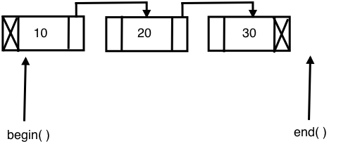
The STL's forward_list container is built on top of a singly linked list data structure; hence, it only supports navigation in the forward direction. As forward_list consumes one less pointer for every node in terms of memory and runtime, it is considered more efficient compared with the list container. However, as price for the extra edge of performance advantage, forward_list had to give up some functionalities.
The following diagram shows the internal data-structure used in forward_list:
Let's explore the following sample code:
#include <iostream>
#include <forward_list>
#include <iterator>
#include <algorithm>
using namespace std;

int main ( ) {

  forward_list<int> l = { 10, 10, 20, 30, 45, 45, 50 };

  cout << "nlist with all values ..." << endl;
  copy ( l.begin(), l.end(), ostream_iterator<int>(cout, "t") );

  cout << "nSize of list with duplicates is " << distance( l.begin(), l.end() ) << endl;

  l.unique();

  cout << "nSize of list without duplicates is " << distance( l.begin(), l.end() ) << endl;

  l.resize( distance( l.begin(), l.end() ) );

  cout << "nlist after removing duplicates ..." << endl;
  copy ( l.begin(), l.end(), ostream_iterator<int>(cout, "t") );
  cout << endl;

  return 0;

}
The output can be viewed with the following command:
./a.out
The output will be as follows:
list with all values ...
10    10    20    30    45    45    50
Size of list with duplicates is 7

Size of list without duplicates is 5

list after removing duplicates ...
10    20   30   45   50
The following code declares and initializes the forward_list container with some unique values and some duplicate values:
forward_list<int> l = { 10, 10, 20, 30, 45, 45, 50 };
As the forward_list container doesn't support the size() function, we used the distance() function to find the size of the list:
cout << "nSize of list with duplicates is " << distance( l.begin(), l.end() ) << endl;
The following forward_list<int>::unique() function removes the duplicate integers and retains only the unique values:
l.unique();
The following table shows the commonly used forward_list APIs:
|
API |
Description |
|
front() |
This returns the first value stored in the forward_list container |
|
empty() |
This returns true when the forward_list container is empty and false, otherwise |
|
clear() |
This clears all the values stored in forward_list |
|
push_front<data_type>( value ) |
This adds a value to the front of forward_list |
|
merge( list ) |
This merges two sorted forward_list containers with values of the same type |
|
reverse() |
This reverses the forward_list container |
|
unique() |
This removes duplicate values from the forward_list container |
|
sort() |
This sorts the values stored in forward_list |
Let's explore one more example to get a firm understanding of the forward_list container:
#include <iostream>
#include <forward_list>
#include <iterator>
#include <algorithm>
using namespace std;

int main () {

    forward_list<int> list1 = { 10, 20, 10, 45, 45, 50, 25 };
    forward_list<int> list2 = { 20, 35, 27, 15, 100, 85, 12, 15 };

    cout << "nFirst list before sorting ..." << endl;
    copy ( list1.begin(), list1.end(), ostream_iterator<int>(cout, "t") );
    cout << endl;

    cout << "nSecond list before sorting ..." << endl;
    copy ( list2.begin(), list2.end(), ostream_iterator<int>(cout, "t") );
    cout << endl;

    list1.sort();
    list2.sort();

    cout << "nFirst list after sorting ..." << endl;
    copy ( list1.begin(), list1.end(), ostream_iterator<int>(cout, "t") );
    cout << endl;

    cout << "nSecond list after sorting ..." << endl;
    copy ( list2.begin(), list2.end(), ostream_iterator<int>(cout, "t") );
    cout << endl;


    list1.merge ( list2 );

    cout << "nMerged list ..." << endl;
    copy ( list1.begin(), list1.end(), ostream_iterator<int>(cout, "t") );

    cout << "nMerged list after removing duplicates ..." << endl;
    list1.unique();
    copy ( list1.begin(), list1.end(), ostream_iterator<int>(cout, "t") );

    return 0;
}
The preceding code snippet is an interesting example that demonstrates the practical use of the sort(), merge(), and unique() STL algorithms.
The output can be viewed with the following command:
./a.out
The output of the program is as follows:
First list before sorting ...
10   20   10   45   45   50   25
Second list before sorting ...
20   35   27   15   100  85   12   15

First list after sorting ...
10   10   20   25   45   45   50
Second list after sorting ...
12   15   15   20   27   35   85   100

Merged list ...
10   10   12   15   15   20   20   25   27   35   45   45  50   85  100
Merged list after removing duplicates ...
10   12   15   20   25   27   35   45   50   85  100
The output and the program are pretty self-explanatory.
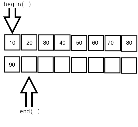
The deque container is a double-ended queue and the data structure used could be a dynamic array or a vector. In a deque, it is possible to insert an element both at the front and back, with a constant time complexity of O(1), unlike vectors, in which the time complexity of inserting an element at the back is O(1) while that for inserting an element at the front is O(N). The deque doesn't suffer from the problem of reallocation, which is suffered by a vector. However, all the benefits of a vector are there with deque, except that deque is slightly better in terms of performance as compared to a vector as there are several rows of dynamic arrays or vectors in each row.
The following diagram shows the internal data structure used in a deque container:
Let's write a simple program to try out the deque container:
#include <iostream>
#include <deque>
#include <algorithm>
#include <iterator>
using namespace std;

int main () {
  deque<int> d = { 10, 20, 30, 40, 50 };

  cout << "nInitial size of deque is " << d.size() << endl;

  d.push_back( 60 );
  d.push_front( 5 );

  cout << "nSize of deque after push back and front is " << d.size() << endl;

  copy ( d.begin(), d.end(), ostream_iterator<int>( cout, "t" ) );
  d.clear();

  cout << "nSize of deque after clearing all values is " << d.size() <<
endl;

  cout << "nIs the deque empty after clearing values ? " << ( d.empty()
? "true" : "false" ) << endl;

return 0;
}
The output can be viewed with the following command:
./a.out
The output of the program is as follows:
Intitial size of deque is 5

Size of deque after push back and front is 7

Print the deque ...
5  10  20  30  40  50  60
Size of deque after clearing all values is 0

Is the deque empty after clearing values ? true
The following table shows the commonly used deque APIs:
|
API |
Description |
|
at ( int index ) |
This returns the value stored at the indexed position. It throws the std::out_of_range exception if the index is invalid. |
|
operator [ int index ] |
This returns the value stored at the indexed position. It is faster than at( int index ) since no bounds checking is performed by this function. |
|
front() |
This returns the first value stored in the deque. |
|
back() |
This returns the last value stored in the deque. |
|
empty() |
This returns true if the deque is empty and false, otherwise. |
|
size() |
This returns the number of values stored in the deque. |
|
capacity() |
This returns the total capacity of the deque, while size() returns the actual number of values stored in the deque. |
|
clear() |
This clears all the values. |
|
push_back<data_type>( value ) |
This adds a new value at the end of the deque. |
Associative containers store data in a sorted fashion, unlike the sequence containers. Hence, the order in which the data is inserted will not be retained by the associative containers. Associative containers are highly efficient in searching a value with O( log n ) runtime complexity. Every time a new value gets added to the container, the container will reorder the values stored internally if required.
The STL supports the following types of associative containers:
Associative containers organize the data as key-value pairs. The data will be sorted based on the key for random and faster access. Associative containers come in two flavors:
The following associative containers come under ordered containers, as they are ordered/sorted in a particular fashion. Ordered associative containers generally use some form of Binary Search Tree (BST); usually, a red-black tree is used to store the data:
The following associative containers come under unordered containers, as they are not ordered in any particular fashion and they use hash tables:
Let's understand the previously mentioned containers with examples in the following subsections.
A set container stores only unique values in a sorted fashion. A set organizes the values using the value as a key. The set container is immutable, that is, the values stored in a set can't be modified; however, the values can be deleted. A set generally uses a red-black tree data structure, which is a form of balanced BST. The time complexity of set operations are guaranteed to be O ( log N ).
Let's write a simple program using a set:
#include <iostream>
#include <set>
#include <vector>
#include <iterator>
#include <algorithm>
using namespace std;

int main( ) {
    set<int> s1 = { 1, 3, 5, 7, 9 };
    set<int> s2 = { 2, 3, 7, 8, 10 };

    vector<int> v( s1.size() + s2.size() );

    cout << "nFirst set values are ..." << endl;
    copy ( s1.begin(), s1.end(), ostream_iterator<int> ( cout, "t" ) );
    cout << endl;

    cout << "nSecond set values are ..." << endl;
    copy ( s2.begin(), s2.end(), ostream_iterator<int> ( cout, "t" ) );
    cout << endl;

    auto pos = set_difference ( s1.begin(), s1.end(), s2.begin(), s2.end(), v.begin() );
    v.resize ( pos - v.begin() );

    cout << "nValues present in set one but not in set two are ..." << endl;
    copy ( v.begin(), v.end(), ostream_iterator<int> ( cout, "t" ) );
    cout << endl;

    v.clear();

    v.resize ( s1.size() + s2.size() );

    pos = set_union ( s1.begin(), s1.end(), s2.begin(), s2.end(), v.begin() );

    v.resize ( pos - v.begin() );

    cout << "nMerged set values in vector are ..." << endl;
    copy ( v.begin(), v.end(), ostream_iterator<int> ( cout, "t" ) );
    cout << endl;

    return 0;
}
The output can be viewed with the following command:
./a.out
The output of the program is as follows:
First set values are ...
1   3   5   7   9

Second set values are ...
2   3   7   8   10

Values present in set one but not in set two are ...
1   5   9

Merged values of first and second set are ...
1   2   3   5   7   8   9  10
The following code declares and initializes two sets, s1 and s2:
set<int> s1 = { 1, 3, 5, 7, 9 };
set<int> s2 = { 2, 3, 7, 8, 10 };
The following line will ensure that the vector has enough room to store the values in the resultant vector:
vector<int> v( s1.size() + s2.size() );
The following code will print the values in s1 and s2:
cout << "nFirst set values are ..." << endl;
copy ( s1.begin(), s1.end(), ostream_iterator<int> ( cout, "t" ) );
cout << endl;

cout << "nSecond set values are ..." << endl;
copy ( s2.begin(), s2.end(), ostream_iterator<int> ( cout, "t" ) );
cout << endl;
The set_difference() algorithm will populate the vector v with values only present in set s1 but not in s2. The iterator, pos, will point to the last element in the vector; hence, the vector resize will ensure that the extra spaces in the vector are removed:
auto pos = set_difference ( s1.begin(), s1.end(), s2.begin(), s2.end(), v.begin() );
v.resize ( pos - v.begin() );
The following code will print the values populated in the vector v:
cout << "nValues present in set one but not in set two are ..." << endl;
copy ( v.begin(), v.end(), ostream_iterator<int> ( cout, "t" ) );
cout << endl;
The set_union() algorithm will merge the contents of sets s1 and s2 into the vector, and the vector is then resized to fit only the merged values:
pos = set_union ( s1.begin(), s1.end(), s2.begin(), s2.end(), v.begin() );
v.resize ( pos - v.begin() );
The following code will print the merged values populated in the vector v:
cout << "nMerged values of first and second set are ..." << endl;
copy ( v.begin(), v.end(), ostream_iterator<int> ( cout, "t" ) );
cout << endl;
The following table describes the commonly used set APIs:
|
API |
Description |
|
insert( value ) |
This inserts a value into the set |
|
clear() |
This clears all the values in the set |
|
size() |
This returns the total number of entries present in the set |
|
empty() |
This will print true if the set is empty, and returns false otherwise |
|
find() |
This finds the element with the specified key and returns the iterator position |
|
equal_range() |
This returns the range of elements matching a specific key |
|
lower_bound() |
This returns an iterator to the first element not less than the given key |
|
upper_bound() |
This returns an iterator to the first element greater than the given key |
A map stores the values organized by keys. Unlike a set, a map has a dedicated key per value. Maps generally use a red-black tree as an internal data structure, which is a balanced BST that guarantees O( log N ) runtime efficiency for searching or locating a value in the map. The values stored in a map are sorted based on the key, using a red-black tree. The keys used in a map must be unique. A map will not retain the sequences of the input as it reorganizes the values based on the key, that is, the red-black tree will be rotated to balance the red-black tree height.
Let's write a simple program to understand map usage:
#include <iostream>
#include <map>
#include <iterator>
#include <algorithm>
using namespace std;
int main ( ) {

  map<string, long> contacts;

  contacts["Jegan"] = 123456789;
  contacts["Meena"] = 523456289;
  contacts["Nitesh"] = 623856729;
  contacts["Sriram"] = 993456789;

  auto pos = contacts.find( "Sriram" );

  if ( pos != contacts.end() )
    cout << pos->second << endl;

  return 0;
}
Let's compile and check the output of the program:
g++ main.cpp -std=c++17
./a.out
The output is as follows:
Mobile number of Sriram is 8901122334
The following line declares a map with a string name as the key and a long mobile number as the value stored in the map:
map< string, long > contacts;
The following code snippet adds four contacts organized by name as the key:
 contacts[ "Jegan" ] = 1234567890;
 contacts[ "Meena" ] = 5784433221;
 contacts[ "Nitesh" ] = 4567891234;
 contacts[ "Sriram" ] = 8901122334;
The following line will try to locate the contact with the name, Sriram, in the contacts map; if Sriram is found, then the find() function will return the iterator pointing to the location of the key-value pair; otherwise it returns the contacts.end() position:
auto pos = contacts.find( "Sriram" );
The following code verifies whether the iterator, pos, has reached contacts.end() and prints the contact number. Since the map is an associative container, it stores a key=>value pair; hence, pos->first indicates the key and pos->second indicates the value:
 if ( pos != contacts.end() )
      cout << "nMobile number of " << pos->first << " is " << pos->second << endl;
 else
      cout << "nContact not found." << endl;
The following table shows the commonly used map APIs:
|
API |
Description |
|
at ( key ) |
This returns the value for the corresponding key if the key is found; otherwise it throws the std::out_of_range exception |
|
operator[ key ] |
This updates an existing value for the corresponding key if the key is found; otherwise it will add a new entry with the respective key=>value supplied |
|
empty() |
This returns true if the map is empty, and false otherwise |
|
size() |
This returns the count of the key=>value pairs stored in the map |
|
clear() |
This clears the entries stored in the map |
|
count() |
This returns the number of elements matching the given key |
|
find() |
This finds the element with the specified key |
A multiset container works in a manner similar to a set container, except for the fact that a set allows only unique values to be stored whereas a multiset lets you store duplicate values. As you know, in the case of set and multiset containers, the values themselves are used as keys to organize the data. A multiset container is just like a set; it doesn't allow modifying the values stored in the multiset.
Let's write a simple program using a multiset:
#include <iostream>
#include <set>
#include <iterator>
#include <algorithm>
using namespace std;

int main() {
  multiset<int> s = { 10, 30, 10, 50, 70, 90 };

  cout << "nMultiset values are ..." << endl;

  copy ( s.begin(), s.end(), ostream_iterator<int> ( cout, "t" ) );
  cout << endl;

  return 0;
}
The output can be viewed with the following command:
./a.out
The output of the program is as follows:
Multiset values are ...
10 30 10 50 70 90
Interestingly, in the preceding output, you can see that the multiset holds duplicate values.
A multimap works exactly as a map, except that a multimap container will allow multiple values to be stored with the same key.
Let's explore the multimap container with a simple example:
#include <iostream>
#include <map>
#include <vector>
#include <iterator>
#include <algorithm>
using namespace std;

int main() {
  multimap< string, long > contacts = {
    { "Jegan", 2232342343 },
    { "Meena", 3243435343 },
    { "Nitesh", 6234324343 },
    { "Sriram", 8932443241 },
    { "Nitesh", 5534327346 }
  };

  auto pos = contacts.find ( "Nitesh" );
  int count = contacts.count( "Nitesh" );
  int index = 0;

  while ( pos != contacts.end() ) {
  cout << "\nMobile number of " << pos->first << " is " <<
  pos->second << endl;
  ++index;
  ++pos;
  if ( index == count )
     break;
}
  return 0;
}
The program can be compiled and the output can be viewed with the following commands:
g++ main.cpp -std=c++17

./a.out
The output of the program is as follows:
Mobile number of Nitesh is 6234324343
Mobile number of Nitesh is 5534327346
An unordered set works in a manner similar to a set, except that the internal behavior of these containers differs. A set makes use of red-black trees while an unordered set makes use of hash tables. The time complexity of set operations is O( log N) while the time complexity of unordered set operations is O(1); hence, the unordered set tends to be faster than the set.
The values stored in an unordered set are not organized in any particular fashion, unlike in a set, which stores values in a sorted fashion. If performance is the criteria, then an unordered set is a good bet; however, if iterating the values in a sorted fashion is a requirement, then set is a good choice.
An unordered map works in a manner similar to a map, except that the internal behavior of these containers differs. A map makes use of red-black trees while unordered map makes use of hash tables. The time complexity of map operations is O( log N) while that of unordered map operations is O(1); hence, an unordered map tends to be faster than a map.
The values stored in an unordered map are not organized in any particular fashion, unlike in a map where values are sorted by keys.
An unordered multiset works in a manner similar to a multiset, except that the internal behavior of these containers differs. A multiset makes use of red-black trees while an unordered multiset makes use of hash tables. The time complexity of multiset operations is O( log N) while that of unordered multiset operations is O(1). Hence, an unordered multiset tends to be faster than a multiset.
The values stored in an unordered multiset are not organized in any particular fashion, unlike in a multiset where values are stored in a sorted fashion. If performance is the criteria, unordered multisets are a good bet; however, if iterating the values in a sorted fashion is a requirement, then multiset is a good choice.
An unordered multimap works in a manner similar to a multimap, except that the internal behavior of these containers differs. A multimap makes use of red-black trees while an unordered multimap makes use of hash tables. The time complexity of multimap operations is O( log N) while that of unordered multimap operations is O(1); hence, an unordered multimap tends to be faster than a multimap.
The values stored in an unordered multimap are not organized in any particular fashion, unlike in multimaps where values are sorted by keys. If performance is the criteria, then an unordered multimap is a good bet; however, if iterating the values in a sorted fashion is a requirement, then multimap is a good choice.
Container adapters adapt existing containers to provide new containers. In simple terms, STL extension is done with composition instead of inheritance.
STL containers can't be extended by inheritance, as their constructors aren't virtual. Throughout the STL, you can observe that while static polymorphism is used both in terms of operator overloading and templates, dynamic polymorphism is consciously avoided for performance reasons. Hence, extending the STL by subclassing the existing containers isn't a good idea, as it would lead to memory leaks because container classes aren't designed to behave like base classes.
The STL supports the following container adapters:
Let's explore the container adapters in the following subsections.
Stack is not a new container; it is a template adapter class. The adapter containers wrap an existing container and provide high-level functionalities. The stack adapter container offers stack operations while hiding the unnecessary functionalities that are irrelevant for a stack. The STL stack makes use of a deque container by default; however, we can instruct the stack to use any existing container that meets the requirement of the stack during the stack instantiation.
Deques, lists, and vectors meet the requirements of a stack adapter.
A stack operates on the Last In First Out (LIFO) philosophy.
The following table shows commonly used stack APIs:
|
API |
Description |
|
top() |
This returns the top-most value in the stack, that is, the value that was added last |
|
push<data_type>( value ) |
This will push the value provided to the top of the stack |
|
pop() |
This will remove the top-most value from the stack |
|
size() |
This returns the number of values present in the stack |
|
empty() |
This returns true if the stack is empty; otherwise it returns false |
It's time to get our hands dirty; let's write a simple program to use a stack:
#include <iostream>
#include <stack>
#include <iterator>
#include <algorithm>
using namespace std;

int main ( ) {

  stack<string> spoken_languages;

  spoken_languages.push ( "French" );
  spoken_languages.push ( "German" );
  spoken_languages.push ( "English" );
  spoken_languages.push ( "Hindi" );
  spoken_languages.push ( "Sanskrit" );
  spoken_languages.push ( "Tamil" );

  cout << "nValues in Stack are ..." << endl;
  while ( ! spoken_languages.empty() ) {
              cout << spoken_languages.top() << endl;
        spoken_languages.pop();
  }
  cout << endl;


  return 0;
}
The program can be compiled and the output can be viewed with the following command:
g++ main.cpp -std=c++17

./a.out
The output of the program is as follows:
Values in Stack are ...
Tamil
Kannada
Telugu
Sanskrit
Hindi
English
German
French
From the preceding output, we can see the LIFO behavior of stack.
A queue works based on the First In First Out (FIFO) principle. A queue is not a new container; it is a templatized adapter class that wraps an existing container and provides the high-level functionalities that are required for queue operations, while hiding the unnecessary functionalities that are irrelevant for a queue. The STL queue makes use of a deque container by default; however, we can instruct the queue to use any existing container that meets the requirement of the queue during the queue instantiation.
In a queue, new values can be added at the back and removed from the front. Deques, lists, and vectors meet the requirements of a queue adapter.
The following table shows the commonly used queue APIs:
|
API |
Description |
|
push() |
This appends a new value at the back of the queue |
|
pop() |
This removes the value at the front of the queue |
|
front() |
This returns the value in the front of the queue |
|
back() |
This returns the value at the back of the queue |
|
empty() |
This returns true when the queue is empty; otherwise it returns false |
|
size() |
This returns the number of values stored in the queue |
Let's use a queue in the following program:
#include <iostream>
#include <queue>
#include <iterator>
#include <algorithm>
using namespace std;

int main () {
  queue<int> q;

  q.push ( 100 );
  q.push ( 200 );
  q.push ( 300 );

  cout << "nValues in Queue are ..." << endl;
  while ( ! q.empty() ) {
    cout << q.front() << endl;
    q.pop();
  }

  return 0;
}
The program can be compiled and the output can be viewed with the following commands:
g++ main.cpp -std=c++17

./a.out
The output of the program is as follows:
Values in Queue are ...
100
200
300
From the preceding output, you can observe that the values were popped out in the same sequence that they were pushed in, that is, FIFO.
A priority queue is not a new container; it is a templatized adapter class that wraps an existing container and provides high-level functionalities that are required for priority queue operations, while hiding the unnecessary functionalities that are irrelevant for a priority queue. A priority queue makes use of a vector container by default; however, a deque container also meets the requirement of the priority queue. Hence, during the priority queue instantiation, you could instruct the priority queue to make use of a deque as well.
A priority queue organizes the data in such a way that the highest priority value appears first; in other words, the values are sorted in a descending order.
The deque and vector meet the requirements of a priority queue adaptor.
The following table shows commonly used priority queue APIs:
|
API |
Description |
|
push() |
This appends a new value at the back of the priority queue |
|
pop() |
This removes the value at the front of the priority queue |
|
empty() |
This returns true when the priority queue is empty; otherwise it returns false |
|
size() |
This returns the number of values stored in the priority queue |
|
top() |
This returns the value in the front of the priority queue |
Let's write a simple program to understand priority_queue:
#include <iostream>
#include <queue>
#include <iterator>
#include <algorithm>
using namespace std;

int main () {
  priority_queue<int> q;

  q.push( 100 );
  q.push( 50 );
  q.push( 1000 );
  q.push( 800 );
  q.push( 300 );

  cout << "nSequence in which value are inserted are ..." << endl;
  cout << "100t50t1000t800t300" << endl;
  cout << "Priority queue values are ..." << endl;

  while ( ! q.empty() ) {
    cout << q.top() << "t";
    q.pop();
  }
  cout << endl;

  return 0;
}
The program can be compiled and the output can be viewed with the following command:
g++ main.cpp -std=c++17

./a.out
The output of the program is as follows:
Sequence in which value are inserted are ...
100   50   1000  800   300

Priority queue values are ...
1000  800   300   100   50
From the preceding output, you can observe that priority_queue is a special type of queue that reorders the inputs in such a way that the highest value appears first.
In this chapter you learned about ready-made generic containers, functors, iterators, and algorithms. You also learned set, map, multiset, and multimap associative containers, their internal data structures, and common algorithms that can be applied on them. Further you learned how to use the various containers with practical hands-on code samples.
In the next chapter, you will learn template programming, which helps you master the essentials of templates.
In this chapter, we will cover the following topics:
Let's now start learning generic programming.
Generic programming is a style of programming that helps you develop reusable code or generic algorithms that can be applied to a wide variety of data types. Whenever a generic algorithm is invoked, the data types will be supplied as parameters with a special syntax.
Let's say we would like to write a sort() function, which takes an array of inputs that needs to be sorted in an ascending order. Secondly, we need the sort() function to sort int, double, char, and string data types. There are a couple of ways this can be solved:
Well, both approaches have their own merits and demerits. The advantage of the first approach is that, since there are dedicated functions for the int, double, char, and string data types, the compiler will be able to perform type checking if an incorrect data type is supplied. The disadvantage of the first approach is that we have to write four different functions even though the logic remains the same across all the functions. If a bug is identified in the algorithm, it must be fixed separately in all four functions; hence, heavy maintenance efforts are required. If we need to support another data type, we will end up writing one more function, and this will keep growing as we need to support more data types.
The advantage of the second approach is that we could just write one macro for all the data types. However, one very discouraging disadvantage is that the compiler will not be able to perform type checking, and this approach is more prone to errors and may invite many unexpected troubles. This approach is dead against object-oriented coding principles.
C++ supports generic programming with templates, which has the following benefits:
However, the disadvantages are as follows:
A function template lets you parameterize a data type. The reason this is referred to as generic programming is that a single template function will support many built-in and user-defined data types. A templatized function works like a C-style macro, except for the fact that the C++ compiler will type check the function when we supply an incompatible data type at the time of invoking the template function.
It will be easier to understand the template concept with a simple example, as follows:
#include <iostream>
#include <algorithm>
#include <iterator>
using namespace std;

template <typename T, int size>
void sort ( T input[] ) {

     for ( int i=0; i<size; ++i) {
         for (int j=0; j<size; ++j) {
              if ( input[i] < input[j] )
                  swap (input[i], input[j] );
         }
     }

}

int main () {
        int a[10] = { 100, 10, 40, 20, 60, 80, 5, 50, 30, 25 };

        cout << "nValues in the int array before sorting ..." << endl;
        copy ( a, a+10, ostream_iterator<int>( cout, "t" ) );
        cout << endl;

        ::sort<int, 10>( a );

        cout << "nValues in the int array after sorting ..." << endl;
        copy ( a, a+10, ostream_iterator<int>( cout, "t" ) );
        cout << endl;

        double b[5] = { 85.6d, 76.13d, 0.012d, 1.57d, 2.56d };

        cout << "nValues in the double array before sorting ..." << endl;
        copy ( b, b+5, ostream_iterator<double>( cout, "t" ) );
        cout << endl;


        ::sort<double, 5>( b );

        cout << "nValues in the double array after sorting ..." << endl;
        copy ( b, b+5, ostream_iterator<double>( cout, "t" ) );
        cout << endl;

        string names[6] = {
               "Rishi Kumar Sahay",
               "Arun KR",
               "Arun CR",
               "Ninad",
               "Pankaj",
               "Nikita"
        };

        cout << "nNames before sorting ..." << endl;
        copy ( names, names+6, ostream_iterator<string>( cout, "n" ) );
        cout << endl;

        ::sort<string, 6>( names );

        cout << "nNames after sorting ..." << endl;
        copy ( names, names+6, ostream_iterator<string>( cout, "n" ) );
        cout << endl;

        return 0;
}
Run the following commands:
g++ main.cpp -std=c++17
./a.out
The output of the preceding program is as follows:
Values in the int array before sorting ...
100  10   40   20   60   80   5   50   30   25

Values in the int array after sorting ...
5    10   20   25   30   40   50   60   80   100

Values in the double array before sorting ...
85.6d 76.13d 0.012d 1.57d 2.56d

Values in the double array after sorting ...
0.012   1.57   2.56   76.13   85.6

Names before sorting ...
Rishi Kumar Sahay
Arun KR
Arun CR
Ninad
Pankaj
Nikita

Names after sorting ...
Arun CR
Arun KR
Nikita
Ninad
Pankaj
Rich Kumar Sahay
Isn't it really interesting to see just one template function doing all the magic? Yes, that's how cool C++ templates are!
The following code defines a function template. The keyword, template <typename T, int size>, tells the compiler that what follows is a function template:
template <typename T, int size>
void sort ( T input[] ) {

 for ( int i=0; i<size; ++i) {
     for (int j=0; j<size; ++j) {
         if ( input[i] < input[j] )
             swap (input[i], input[j] );
     }
 }

}
The line, void sort ( T input[] ), defines a function named sort, which returns void and receives an input array of type T. The T type doesn't indicate any specific data type. T will be deduced at the time of instantiating the function template during compile time.
The following code populates an integer array with some unsorted values and prints the same to the terminal:
 int a[10] = { 100, 10, 40, 20, 60, 80, 5, 50, 30, 25 };
 cout << "nValues in the int array before sorting ..." << endl;
 copy ( a, a+10, ostream_iterator<int>( cout, "t" ) );
 cout << endl;
The following line will instantiate an instance of a function template for the int data type. At this point, typename T is substituted and a specialized function is created for the int data type. The scope-resolution operator in front of sort, that is, ::sort(), ensures that it invokes our custom function, sort(), defined in the global namespace; otherwise, the C++ compiler will attempt to invoke the sort() algorithm defined in the std namespace, or from any other namespace if such a function exists. The <int, 10> variable tells the compiler to create an instance of a function, substituting typename T with int, and 10 indicates the size of the array used in the template function:
::sort<int, 10>( a );
The following lines will instantiate two additional instances that support a double array of 5 elements and a string array of 6 elements respectively:
::sort<double, 5>( b );
::sort<string, 6>( names );
If you are curious to know some more details about how the C++ compiler instantiates the function templates to support int, double, and string, you could try the Unix utilities, nm and c++filt. The nm Unix utility will list the symbols in the symbol table, as follows:
nm ./a.out | grep sort

00000000000017f1 W _Z4sortIdLi5EEvPT_
0000000000001651 W _Z4sortIiLi10EEvPT_
000000000000199b W _Z4sortINSt7__cxx1112basic_stringIcSt11char_traitsIcESaIcEEELi6EEvPT_
As you can see, there are three different overloaded sort functions in the binary; however, we have defined only one template function. As the C++ compiler has mangled names to deal with function overloading, it is difficult for us to interpret which function among the three functions is meant for the int, double, and string data types.
However, there is a clue: the first function is meant for double, the second is meant for int, and the third is meant for string. The name-mangled function has _Z4sortIdLi5EEvPT_ for double, _Z4sortIiLi10EEvPT_ for int, and _Z4sortINSt7__cxx1112basic_stringIcSt11char_traitsIcESaIcEEELi6EEvPT_ for string. There is another cool Unix utility to help you interpret the function signatures without much struggle. Check the following output of the c++filt utility:
c++filt _Z4sortIdLi5EEvPT_
void sort<double, 5>(double*)

c++filt _Z4sortIiLi10EEvPT_
void sort<int, 10>(int*)

c++filt _Z4sortINSt7__cxx1112basic_stringIcSt11char_traitsIcESaIcEEELi6EEvPT_
void sort<std::__cxx11::basic_string<char, std::char_traits<char>, std::allocator<char> >, 6>(std::__cxx11::basic_string<char, std::char_traits<char>, std::allocator<char> >*)
Hopefully, you will find these utilities useful while working with C++ templates. I'm sure these tools and techniques will help you to debug any C++ application.
Overloading function templates works exactly like regular function overloading in C++. However, I'll help you recollect the C++ function overloading basics.
The function overloading rules and expectations from the C++ compiler are as follows:
If any of these aforementioned rules aren't met, the C++ compiler will not treat them as overloaded functions. If there is any ambiguity in differentiating between the overloaded functions, the C++ compiler will report it promptly as a compilation error.
It is time to explore this with an example, as shown in the following program:
#include <iostream>
#include <array>
using namespace std;

void sort ( array<int,6> data ) {


     cout << "Non-template sort function invoked ..." << endl;

     int size = data.size();

     for ( int i=0; i<size; ++i ) {
          for ( int j=0; j<size; ++j ) {
                if ( data[i] < data[j] )
                    swap ( data[i], data[j] );
          }
     }

}

template <typename T, int size>
void sort ( array<T, size> data ) {

     cout << "Template sort function invoked with one argument..." << endl;

     for ( int i=0; i<size; ++i ) {
         for ( int j=0; j<size; ++j ) {
             if ( data[i] < data[j] )
                swap ( data[i], data[j] );
         }
     }

}

template <typename T>
void sort ( T data[], int size ) {
     cout << "Template sort function invoked with two arguments..." << endl;

     for ( int i=0; i<size; ++i ) {
         for ( int j=0; j<size; ++j ) {
             if ( data[i] < data[j] )
                swap ( data[i], data[j] );
         }
     }

}

int main() {

    //Will invoke the non-template sort function
    array<int, 6> a = { 10, 50, 40, 30, 60, 20 };
    ::sort ( a );

    //Will invoke the template function that takes a single argument
    array<float,6> b = { 10.6f, 57.9f, 80.7f, 35.1f, 69.3f, 20.0f };
    ::sort<float,6>( b );

    //Will invoke the template function that takes a single argument
    array<double,6> c = { 10.6d, 57.9d, 80.7d, 35.1d, 69.3d, 20.0d };
    ::sort<double,6> ( c );

    //Will invoke the template function that takes two arguments
    double d[] = { 10.5d, 12.1d, 5.56d, 1.31d, 81.5d, 12.86d };
    ::sort<double> ( d, 6 );

    return 0;

}
Run the following commands:
g++ main.cpp -std=c++17

./a.out
The output of the preceding program is as follows:
Non-template sort function invoked ...

Template sort function invoked with one argument...

Template sort function invoked with one argument...

Template sort function invoked with two arguments...
The following code is a non-template version of our custom sort() function:
void sort ( array<int,6> data ) {

     cout << "Non-template sort function invoked ..." << endl;

     int size = data.size();

     for ( int i=0; i<size; ++i ) {
         for ( int j=0; j<size; ++j ) {
             if ( data[i] < data[j] )
                 swap ( data[i], data[j] );
         }
     }

}
Non-template functions and template functions can coexist and participate in function overloading. One weird behavior of the preceding function is that the size of the array is hardcoded.
The second version of our sort() function is a template function, as shown in the following code snippet. Interestingly, the weird issue that we noticed in the first non-template sort() version is addressed here:
template <typename T, int size>
void sort ( array<T, size> data ) {

     cout << "Template sort function invoked with one argument..." << endl;

     for ( int i=0; i<size; ++i ) {
         for ( int j=0; j<size; ++j ) {
             if ( data[i] < data[j] )
                swap ( data[i], data[j] );
         }
     }

}
In the preceding code, both the data type and the size of the array are passed as template arguments, which are then passed to the function call arguments. This approach makes the function generic, as this function can be instantiated for any data type.
The third version of our custom sort() function is also a template function, as shown in the following code snippet:
template <typename T>
void sort ( T data[], int size ) {

     cout << "Template sort function invoked with two argument..." << endl;

     for ( int i=0; i<size; ++i ) {
         for ( int j=0; j<size; ++j ) {
             if ( data[i] < data[j] )
                swap ( data[i], data[j] );
         }
     }

}
The preceding template function takes a C-style array; hence, it also expects the user to indicate its size. However, the size of the array could be computed within the function, but for demonstration purposes, I need a function that takes two arguments. The previous function isn't recommended, as it uses a C-style array; ideally, we would use one of the STL containers.
Now, let's understand the main function code. The following code declares and initializes the STL array container with six values, which is then passed to our sort() function defined in the default namespace:
 //Will invoke the non-template sort function
 array<int, 6> a = { 10, 50, 40, 30, 60, 20 };
 ::sort ( a );
The preceding code will invoke the non-template sort() function. An important point to note is that, whenever C++ encounters a function call, it first looks for a non-template version; if C++ finds a matching non-template function version, its search for the correct function definition ends there. If the C++ compiler isn't able to identify a non-template function definition that matches the function call signature, then it starts looking for any template function that could support the function call and instantiates a specialized function for the data type required.
Let's understand the following code:
//Will invoke the template function that takes a single argument
array<float,6> b = { 10.6f, 57.9f, 80.7f, 35.1f, 69.3f, 20.0f };
::sort<float,6>( b );
This will invoke the template function that receives a single argument. As there is no non-template sort() function that receives an array<float,6> data type, the C++ compiler will instantiate such a function out of our user-defined sort() template function with a single argument that takes array<float, 6>.
In the same way, the following code triggers the compiler to instantiate a double version of the template sort() function that receives array<double, 6>:
  //Will invoke the template function that takes a single argument
 array<double,6> c = { 10.6d, 57.9d, 80.7d, 35.1d, 69.3d, 20.0d };
 ::sort<double,6> ( c );
Finally, the following code will instantiate an instance of the template sort() that receives two arguments and invokes the function:
 //Will invoke the template function that takes two arguments
 double d[] = { 10.5d, 12.1d, 5.56d, 1.31d, 81.5d, 12.86d };
 ::sort<double> ( d, 6 );
If you have come this far, I'm sure you like the C++ template topics discussed so far.
C++ templates extend the function template concepts to classes too, and enable us to write object-oriented generic code. In the previous sections, you learned the use of function templates and overloading. In this section, you will learn writing template classes that open up more interesting generic programming concepts.
A class template lets you parameterize the data type on the class level via a template type expression.
Let's understand a class template with the following example:
//myalgorithm.h
#include <iostream>
#include <algorithm>
#include <array>
#include <iterator>
using namespace std;

template <typename T, int size>
class MyAlgorithm {

public:
        MyAlgorithm() { }
        ~MyAlgorithm() { }


        void sort( array<T, size> &data ) {
             for ( int i=0; i<size; ++i ) {
                 for ( int j=0; j<size; ++j ) {
                     if ( data[i] < data[j] )
                         swap ( data[i], data[j] );
                 }
             }
        }

        void sort ( T data[size] );

};

template <typename T, int size>
inline void MyAlgorithm<T, size>::sort ( T data[size] ) {
       for ( int i=0; i<size; ++i ) {
           for ( int j=0; j<size; ++j ) {
               if ( data[i] < data[j] )
                  swap ( data[i], data[j] );
           }
       }
}
Let's use myalgorithm.h in the following main.cpp program as follows:
#include "myalgorithm.h"

int main() {

    MyAlgorithm<int, 10> algorithm1;

    array<int, 10> a = { 10, 5, 15, 20, 25, 18, 1, 100, 90, 18 };

    cout << "nArray values before sorting ..." << endl;
    copy ( a.begin(), a.end(), ostream_iterator<int>(cout, "t") );
    cout << endl;

    algorithm1.sort ( a );

    cout << "nArray values after sorting ..." << endl;
    copy ( a.begin(), a.end(), ostream_iterator<int>(cout, "t") );
    cout << endl;

    MyAlgorithm<int, 10> algorithm2;
    double d[] = { 100.0, 20.5, 200.5, 300.8, 186.78, 1.1 };

    cout << "nArray values before sorting ..." << endl;
    copy ( d.begin(), d.end(), ostream_iterator<double>(cout, "t") );
    cout << endl;

    algorithm2.sort ( d );

    cout << "nArray values after sorting ..." << endl;
    copy ( d.begin(), d.end(), ostream_iterator<double>(cout, "t") );
    cout << endl;

    return 0;

}
Let's quickly compile the program using the following command:
g++ main.cpp -std=c++17

./a.out
The output is as follows:
Array values before sorting ...
10  5   15   20   25   18   1   100   90   18

Array values after sorting ...
1   5   10   15   18   18   20   25   90   100

Array values before sorting ...
100   20.5   200.5   300.8   186.78   1.1

Array values after sorting ...
1.1     20.5   100   186.78  200.5  300.8
The following code declares a class template. The keyword, template <typename T, int size>, can be replaced with <class T, int size>. Both keywords can be interchanged in function and class templates; however, as an industry best practice, template<class T> can be used only with class templates to avoid confusion:
template <typename T, int size>
class MyAlgorithm
One of the overloaded sort() methods is defined inline as follows:
 void sort( array<T, size> &data ) {
      for ( int i=0; i<size; ++i ) {
          for ( int j=0; j<size; ++j ) {
              if ( data[i] < data[j] )
                 swap ( data[i], data[j] );
          }
      }
 }
The second overloaded sort() function is just declared within the class scope, without any definition, as follows:
template <typename T, int size>
class MyAlgorithm {
      public:
           void sort ( T data[size] );
};
The preceding sort() function is defined outside the class scope, as shown in the following code snippet. The weird part is that we need to repeat the template parameters for every member function that is defined outside the class template:
template <typename T, int size>
inline void MyAlgorithm<T, size>::sort ( T data[size] ) {
       for ( int i=0; i<size; ++i ) {
           for ( int j=0; j<size; ++j ) {
               if ( data[i] < data[j] )
                  swap ( data[i], data[j] );
           }
       }
}
Otherwise, the class template concepts remain the same as that of function templates.
So far in this chapter, you have learned how to do generic programming with function templates and class templates. As you understand the class template, a single template class can support any built-in and user-defined data types. However, there are times when we need to treat certain data types with some special treatment with respect to the other data types. In such cases, C++ offers us explicit class specialization support to handle selective data types with differential treatment.
Consider the STL deque container; though deque looks fine for storing, let's say, string, int, double, and long, if we decide to use deque to store a bunch of boolean types, the bool data type takes at least one byte, while it may vary as per compiler vendor implementation. While a single bit can efficiently represent true or false, a boolean at least takes one byte, that is, 8 bits, and the remaining 7 bits are not used. This may appear as though it's okay; however, if you have to store a very large deque of booleans, it definitely doesn't appear to be an efficient idea, right? You may think, what's the big deal? We could write another specialized class or template class for bool. But this approach requires end users to use different classes for different data types explicitly, and this doesn't sound like a good design either, right? This is exactly where C++'s explicit class specialization comes in handy.
Never mind if you aren't convinced yet; the following example will help you understand the need for explicit class specialization and how explicit class specialization works.
Let us develop a DynamicArray class to support a dynamic array of any data type. Let's start with a class template, as shown in the following program:
#include <iostream>
#include <deque>
#include <algorithm>
#include <iterator>
using namespace std;

template < class T >
class DynamicArray {
      private:
           deque< T > dynamicArray;
           typename deque< T >::iterator pos;

      public:
           DynamicArray() { initialize(); }
           ~DynamicArray() { }

           void initialize() {
                 pos = dynamicArray.begin();
           }

           void appendValue( T element ) {
                 dynamicArray.push_back ( element );
           }

           bool hasNextValue() {
                 return ( pos != dynamicArray.end() );
           }

           T getValue() {
                 return *pos++;
           }

};
The preceding DynamicArray template class internally makes use of the STL deque class. Hence, you could consider the DynamicArray template class a custom adapter container. Let's explore how the DynamicArray template class can be used in main.cpp with the following code snippet:
#include "dynamicarray.h"
#include "dynamicarrayforbool.h"

int main () {

    DynamicArray<int> intArray;

    intArray.appendValue( 100 );
    intArray.appendValue( 200 );
    intArray.appendValue( 300 );
    intArray.appendValue( 400 );

    intArray.initialize();

    cout << "nInt DynamicArray values are ..." << endl;
    while ( intArray.hasNextValue() )
          cout << intArray.getValue() << "t";
    cout << endl;

    DynamicArray<char> charArray;
    charArray.appendValue( 'H' );
    charArray.appendValue( 'e' );
    charArray.appendValue( 'l' );
    charArray.appendValue( 'l' );
    charArray.appendValue( 'o' );

    charArray.initialize();

    cout << "nChar DynamicArray values are ..." << endl;
    while ( charArray.hasNextValue() )
          cout << charArray.getValue() << "t";
    cout << endl;

    DynamicArray<bool> boolArray;

    boolArray.appendValue ( true );
    boolArray.appendValue ( false );
    boolArray.appendValue ( true );
    boolArray.appendValue ( false );

    boolArray.initialize();

    cout << "nBool DynamicArray values are ..." << endl;
    while ( boolArray.hasNextValue() )
         cout << boolArray.getValue() << "t";
    cout << endl;

    return 0;

}
Let's quickly compile the program using the following command:
g++ main.cpp -std=c++17

./a.out
The output is as follows:
Int DynamicArray values are ...
100   200   300   400

Char DynamicArray values are ...
H   e   l   l   o

Bool DynamicArray values are ...
1   0   1   0
Great! Our custom adapter container seems to work fine.
Let's zoom in and try to understand how the previous program works. The following code tells the C++ compiler that what follows is a class template:
template < class T >
class DynamicArray {
      private:
           deque< T > dynamicArray;
           typename deque< T >::iterator pos;
As you can see, the DynamicArray class makes use of STL deque internally, and an iterator for deque is declared with the name, pos. This iterator, pos, is utilized by the Dynamic template class to provide high-level methods such as the initialize(), appendValue(), hasNextValue(), and getValue() methods.
The initialize() method initializes the deque iterator pos to the first data element stored within deque. The appendValue( T element ) method lets you add a data element at the end of deque. The hasNextValue() method tells whether the DynamicArray class has further data values stored--true indicates it has further values and false indicates that the DynamicArray navigation has reached the end of deque. The initialize() method can be used to reset the pos iterator to the starting point when required. The getValue() method returns the data element pointed by the pos iterator at that moment. The getValue() method doesn't perform any validation; hence, it must be combined with hasNextValue() before invoking getValue() to safely access the values stored in DynamicArray.
Now, let's understand the main() function. The following code declares a DynamicArray class that stores the int data type; DynamicArray<int> intArray will trigger the C++ compiler to instantiate a DynamicArray class that is specialized for the int data type:
DynamicArray<int> intArray;

intArray.appendValue( 100 );
intArray.appendValue( 200 );
intArray.appendValue( 300 );
intArray.appendValue( 400 );
The values 100, 200, 300, and 400 are stored back to back within the DynamicArray class. The following code ensures that the intArray iterator points to the first element. Once the iterator is initialized, the values stored in the DynamicArray class are printed with the getValue() method, while hasNextValue() ensures that the navigation hasn't reached the end of the DynamicArray class:
intArray.initialize();
cout << "nInt DynamicArray values are ..." << endl;
while ( intArray.hasNextValue() )
      cout << intArray.getValue() << "t";
cout << endl;
Along the same lines, in the main function, a char DynamicArray class is created, populated with some data, and printed. Let's skip char DynamicArray and directly move on to the DynamicArray class that stores bool.
DynamicArray<bool> boolArray;

boolArray.appendValue ( "1010" );

boolArray.initialize();

cout << "nBool DynamicArray values are ..." << endl;

while ( boolArray.hasNextValue() )
      cout << boolArray.getValue() << "t";
cout << endl;
From the preceding code snippet, we can see everything looks okay, right? Yes, the preceding code works perfectly fine; however, there is a performance issue with the DynamicArray design approach. While true can be represented by 1 and false can be represented by 0, which requires just 1 bit, the preceding DynamicArray class makes use of 8 bits to represent 1 and 8 bits to represent 0, which we must fix without forcing end users to choose a different DynamicArray class that works efficiently for bool.
Let's fix the issue by using explicit class template specialization with the following code:
#include <iostream>
#include <bitset>
#include <algorithm>
#include <iterator>
using namespace std;

template <>
class DynamicArray<bool> {
      private:
          deque< bitset<8> *> dynamicArray;
          bitset<8> oneByte;
          typename deque<bitset<8> * >::iterator pos;
          int bitSetIndex;

          int getDequeIndex () {
              return (bitSetIndex) ? (bitSetIndex/8) : 0;
          }
      public:
          DynamicArray() {
              bitSetIndex = 0;
              initialize();
          }

         ~DynamicArray() { }

         void initialize() {
              pos = dynamicArray.begin();
              bitSetIndex = 0;
         }

         void appendValue( bool value) {
              int dequeIndex = getDequeIndex();
              bitset<8> *pBit = NULL;

              if ( ( dynamicArray.size() == 0 ) || ( dequeIndex >= ( dynamicArray.size()) ) ) {
                   pBit = new bitset<8>();
                   pBit->reset();
                   dynamicArray.push_back ( pBit );
              }

              if ( !dynamicArray.empty() )
                   pBit = dynamicArray.at( dequeIndex );

              pBit->set( bitSetIndex % 8, value );
              ++bitSetIndex;
         }

         bool hasNextValue() {
              return (bitSetIndex < (( dynamicArray.size() * 8 ) ));
         }

         bool getValue() {
              int dequeIndex = getDequeIndex();

              bitset<8> *pBit = dynamicArray.at(dequeIndex);
              int index = bitSetIndex % 8;
              ++bitSetIndex;

              return (*pBit)[index] ? true : false;
         }
};
Did you notice the template class declaration? The syntax for template class specialization is template <> class DynamicArray<bool> { };. The class template expression is empty <> and the name of the class template that works for all data types and the name of the class that works the for the bool data type are kept the same with the template expression, <bool>.
If you observe closely, the specialized DynamicArray class for bool internally makes use of deque< bitset<8> >, that is, deque of bitsets of 8 bits, and, when required, deque will automatically allocate more bitset<8> bits. The bitset variable is a memory-efficient STL container that consumes just 1 bit to represent true or false.
Let's take a look at the main function:
#include "dynamicarray.h"
#include "dynamicarrayforbool.h"

int main () {

    DynamicArray<int> intArray;

    intArray.appendValue( 100 );
    intArray.appendValue( 200 );
    intArray.appendValue( 300 );
    intArray.appendValue( 400 );

    intArray.initialize();

    cout << "nInt DynamicArray values are ..." << endl;

    while ( intArray.hasNextValue() )
          cout << intArray.getValue() << "t";
    cout << endl;

    DynamicArray<char> charArray;

    charArray.appendValue( 'H' );
    charArray.appendValue( 'e' );
    charArray.appendValue( 'l' );
    charArray.appendValue( 'l' );
    charArray.appendValue( 'o' );

    charArray.initialize();

    cout << "nChar DynamicArray values are ..." << endl;
    while ( charArray.hasNextValue() )
          cout << charArray.getValue() << "t";
    cout << endl;

    DynamicArray<bool> boolArray;

    boolArray.appendValue ( true );
    boolArray.appendValue ( false );
    boolArray.appendValue ( true );
    boolArray.appendValue ( false );

    boolArray.appendValue ( true );
    boolArray.appendValue ( false );
    boolArray.appendValue ( true );
    boolArray.appendValue ( false );

    boolArray.appendValue ( true );
    boolArray.appendValue ( true);
    boolArray.appendValue ( false);
    boolArray.appendValue ( false );

    boolArray.appendValue ( true );
    boolArray.appendValue ( true);
    boolArray.appendValue ( false);
    boolArray.appendValue ( false );

    boolArray.initialize();


    cout << "nBool DynamicArray values are ..." << endl;
    while ( boolArray.hasNextValue() )
          cout << boolArray.getValue() ;
    cout << endl;

    return 0;

}
With the class template specialization in place, we can observe from the following that the main code seems the same for bool, char, and double, although the primary template class, DynamicArray, and the specialized DynamicArray<bool> class are different:
DynamicArray<char> charArray;
charArray.appendValue( 'H' );
charArray.appendValue( 'e' );

charArray.initialize();

cout << "nChar DynamicArray values are ..." << endl;
while ( charArray.hasNextValue() )
cout << charArray.getValue() << "t";
cout << endl;

DynamicArray<bool> boolArray;
boolArray.appendValue ( true );
boolArray.appendValue ( false );

boolArray.initialize();

cout << "nBool DynamicArray values are ..." << endl;
while ( boolArray.hasNextValue() )
      cout << boolArray.getValue() ;
cout << endl;
I'm sure you will find this C++ template specialization feature quite useful.
Unlike explicit template specialization, which replaces the primary template class with its own complete definitions for a specific data type, partial template specialization allows us to specialize a certain subset of template parameters supported by the primary template class, while the other generic types can be the same as the primary template class.
When partial template specialization is combined with inheritance, it can do more wonders, as shown in the following example:
#include <iostream>
using namespace std;

template <typename T1, typename T2, typename T3>
class MyTemplateClass {
public:
     void F1( T1 t1, T2 t2, T3 t3 ) {
          cout << "nPrimary Template Class - Function F1 invoked ..." << endl;
          cout << "Value of t1 is " << t1 << endl;
          cout << "Value of t2 is " << t2 << endl;
          cout << "Value of t3 is " << t3 << endl;
     }

     void F2(T1 t1, T2 t2) {
          cout << "nPrimary Tempalte Class - Function F2 invoked ..." << endl;
          cout << "Value of t1 is " << t1 << endl;
          cout << "Value of t2 is " << 2 * t2 << endl;
     }
};
template <typename T1, typename T2, typename T3>
class MyTemplateClass< T1, T2*, T3*> : public MyTemplateClass<T1, T2, T3> {
      public:
          void F1( T1 t1, T2* t2, T3* t3 ) {
               cout << "nPartially Specialized Template Class - Function F1 invoked ..." << endl;
               cout << "Value of t1 is " << t1 << endl;
               cout << "Value of t2 is " << *t2 << endl;
               cout << "Value of t3 is " << *t3 << endl;
          }
};
The main.cpp file will have the following content:
#include "partiallyspecialized.h"

int main () {
    int x = 10;
    int *y = &x;
    int *z = &x;

    MyTemplateClass<int, int*, int*> obj;
    obj.F1(x, y, z);
    obj.F2(x, x);

    return 0;
}
From the preceding code, you may have noticed that the primary template class name and the partially specialized class name are the same as in the case of full or explicit template class specialization. However, there are some syntactic changes in the template parameter expression. In the case of a complete template class specialization, the template parameter expression will be empty, whereas, in the case of a partially specialized template class, listed appears, as shown in the following:
template <typename T1, typename T2, typename T3>
class MyTemplateClass< T1, T2*, T3*> : public MyTemplateClass<T1, T2, T3> { };
The expression, template<typename T1, typename T2, typename T3>, is the template parameter expression used in the primary class template class, and MyTemplateClass< T1, T2*, T3*> is the partial specialization done by the second class. As you can see, the second class has done some specialization on typename T2 and typename T3, as they are used as pointers in the second class; however, typename T1 is used as is in the second class.
Apart from the facts discussed so far, the second class also inherits the primary template class, which helps the second class reuse the public and protected methods of the primary template class. However, a partial template specialization doesn't stop the specialized class from supporting other functions.
While the F1 function from the primary template class is replaced by the partially specialized template class, it reuses the F2 function from the primary template class via inheritance.
Let's quickly compile the program using the following command:
g++ main.cpp -std=c++17

./a.out
The output of the program is as follows:
Partially Specialized Template Classs - Function F1 invoked ...
Value of t1 is 10
Value of t2 is 10
Value of t3 is 10

Primary Tempalte Class - Function F2 invoked ...
Value of t1 is 10
Value of t2 is 20
I hope that you find the partially specialized template class useful.
In this chapter, you learned the following:
Congrats! Overall, you have a good understanding of C++'s template programming.
In the next chapter, you will learn smart pointers.
In the previous chapter, you learned about template programming and the benefits of generic programming. In this chapter, you will learn about the following smart pointer topics:
Let's explore the memory management facilities offered by C++.
In C++, memory management is generally a responsibility of the software developers. This is because C++ standard does not enforce garbage collection support in C++ compiler; hence, it is left to the compiler vendor's choice. Exceptionally, the Sun C++ compiler comes with a garbage collection library named libgc.
C++ language has many powerful features. Of these, needless to say, pointers is one of the most powerful and useful features. Having said pointers are very useful, they do come with their own weird issues, hence they must be used responsibly. When memory management is not taken seriously or not done quite right, it leads to many issues, including application crashes, core dumps, segmentation faults, intermittent difficulties to debug issues, performance issues, and so on. Dangling pointers or rogue pointers sometimes mess with other unrelated applications while the culprit application executes silently; in fact, the victim application might be blamed many times. The worst part about memory leaks is that at certain times it gets really tricky and even experienced developers end up debugging the victim code for countless hours while the culprit code is left untouched. Effective memory management helps avoid memory leaks and lets you develop high-performance applications that are memory efficient.
As the memory model of every operating system varies, every OS may behave differently at a different point in time for the same memory leak issue. Memory management is a big topic, and C++ offers many ways to do it well. We'll discuss some of the useful techniques in the following sections.
The majority of the C++ developers have something in common: all of us love to code complex stuff. You ask a developer, "Hey dude, would you like to reuse code that already exists and works or would you like to develop one yourself?" Though diplomatically, most developers will say to reuse what is already there when possible, their heart will say, "I wish I could design and develop it myself." Complex data structure and algorithms tend to call for pointers. Raw pointers are really cool to work with until you get into trouble.
Raw pointers must be allocated with memory before use and require deallocation once done; it is that simple. However, things get complicated in a product where pointer allocation may happen in one place and deallocation might happen in yet another place. If memory management decisions aren't made correctly, people may assume it is either the caller or callee's responsibility to free up memory, and at times, the memory may not be freed up from either place. In yet another possibility, chances are that the same pointer is deleted multiples times from different places, which could lead to application crashes. If this happens in a Windows device driver, it will most likely end up in a blue screen of death.
Just imagine, what if there were an application exception and the function that threw the exception had a bunch of pointers that were allocated with memory before the exception occurred? It is anybody's guess: there will be memory leaks.
Let's take a simple example that makes use of a raw pointer:
#include <iostream>
using namespace std;

class MyClass {
      public:
           void someMethod() {

                int *ptr = new int();
                *ptr = 100;
                int result = *ptr / 0;  //division by zero error expected
                delete ptr;

           }
};

int main ( ) {

    MyClass objMyClass;
    objMyClass.someMethod();

    return 0;

}
Now, run the following command:
g++ main.cpp -g -std=c++17
Check out the output of this program:
main.cpp: In member function ‘void MyClass::someMethod()’:
main.cpp:12:21: warning: division by zero [-Wdiv-by-zero]
 int result = *ptr / 0;
Now, run the following command:
./a.out
[1] 31674 floating point exception (core dumped) ./a.out
C++ compiler is really cool. Look at the warning message, it bangs on in regard to pointing out the issue. I love the Linux operating system. Linux is quite smart in finding rogue applications that misbehave, and it knocks them off right on time before they cause any damage to the rest of the applications or the OS. A core dump is actually good, while it is cursed instead of celebrating the Linux approach. Guess what, Microsoft's Windows operating systems are equally smarter. They do bug check when they find some applications doing fishy memory accesses and Windows OS as well supports mini-dumps and full dumps which are equivalent to core dumps in Linux OS.
Let's take a look at the Valgrind tool output to check the memory leak issue:
valgrind --leak-check=full --show-leak-kinds=all ./a.out

==32857== Memcheck, a memory error detector
==32857== Copyright (C) 2002-2015, and GNU GPL'd, by Julian Seward et al.
==32857== Using Valgrind-3.12.0 and LibVEX; rerun with -h for copyright info
==32857== Command: ./a.out
==32857==
==32857==
==32857== Process terminating with default action of signal 8 (SIGFPE)
==32857== Integer divide by zero at address 0x802D82B86
==32857== at 0x10896A: MyClass::someMethod() (main.cpp:12)
==32857== by 0x1088C2: main (main.cpp:24)
==32857==
==32857== HEAP SUMMARY:
==32857== in use at exit: 4 bytes in 1 blocks
==32857== total heap usage: 2 allocs, 1 frees, 72,708 bytes allocated
==32857==
==32857== 4 bytes in 1 blocks are still reachable in loss record 1 of 1
==32857== at 0x4C2E19F: operator new(unsigned long) (in /usr/lib/valgrind/vgpreload_memcheck-amd64-linux.so)
==32857== by 0x108951: MyClass::someMethod() (main.cpp:8)
==32857== by 0x1088C2: main (main.cpp:24)
==32857==
==32857== LEAK SUMMARY:
==32857== definitely lost: 0 bytes in 0 blocks
==32857== indirectly lost: 0 bytes in 0 blocks
==32857== possibly lost: 0 bytes in 0 blocks
==32857== still reachable: 4 bytes in 1 blocks
==32857== suppressed: 0 bytes in 0 blocks
==32857==
==32857== For counts of detected and suppressed errors, rerun with: -v
==32857== ERROR SUMMARY: 0 errors from 0 contexts (suppressed: 0 from 0)
[1] 32857 floating point exception (core dumped) valgrind --leak-check=full --show-leak-kinds=all ./a.out
In this output, if you pay attention to the bold portion of the text, you will notice the Valgrind tool did point out the source code line number that caused this core dump. Line number 12 from the main.cpp file is as follows:
int result = *ptr / 0; //division by zero error expected
The moment the exception occurs at line number 12 in the main.cpp file, the code that appears below the exception will never get executed. At line number 13 in the main.cpp file, there appears a delete statement that will never get executed due to the exception:
delete ptr;
The memory allocated to the preceding raw pointer isn't released as the memory pointed by pointers is not freed up during the stack unwinding process. Whenever an exception is thrown by a function and the exception isn't handled by the same function, stack unwinding is guaranteed. However, only the automatic local variables will be cleaned up during the stack unwinding process, not the memory pointed by the pointers. This results in memory leaks.
This is one of the weird issues invited by the use of raw pointers; there are many other similar scenarios. Hopefully you are convinced now that the thrill of using raw pointers does come at a cost. But the penalty paid isn't really worth it as there are good alternatives available in C++ to deal with this issue. You are right, using a smart pointer is the solution that offers the benefits of using pointers without paying the cost attached to raw pointers.
Hence, smart pointers are the way to use pointers safely in C++.
In C++, smart pointers let you focus on the problem at hand by freeing you from the worries of dealing with custom garbage collection techniques. Smart pointers let you use raw pointers safely. They take the responsibility of cleaning up the memory used by raw pointers.
C++ supports many types of smart pointers that can be used in different scenarios:
The auto_ptr smart pointer was introduced in C++11. An auto_ptr smart pointer helps release the heap memory automatically when it goes out of scope. However, due to the way auto_ptr transfers ownership from one auto_ptr instance to another, it was deprecated and unique_ptr was introduced as its replacement. The shared_ptr smart pointer helps multiple shared smart pointers reference the same object and takes care of the memory management burden. The weak_ptr smart pointer helps resolve memory leak issues that arise due to the use of shared_ptr when there is a cyclic dependency issue in the application design.
There are other types of smart pointers and related stuff that are not so commonly used, and they are listed in the following bullet list. However, I would highly recommend that you explore them on your own as you never know when you will find them useful:
The owner_less smart pointer helps compare two or more smart pointers if they share the same raw pointed object. The enable_shared_from_this smart pointer helps get a smart pointer of the this pointer. The bad_weak_ptr smart pointer is an exception class that implies that shared_ptr was created using an invalid smart pointer. The default_delete smart pointer refers to the default destruction policy used by unique_ptr, which invokes the delete statement, while partial specialization for array types that use delete[] is also supported.
In this chapter, we will explore auto_ptr, shared_ptr, weak_ptr, and unique-ptr one by one.
The auto_ptr smart pointer takes a raw pointer, wraps it, and ensures the memory pointed by the raw pointer is released back whenever the auto_ptr object goes out of scope. At any time, only one auto_ptr smart pointer can point to an object. Hence, whenever one auto_ptr pointer is assigned to another auto_ptr pointer, the ownership gets transferred to the auto_ptr instance that has received the assignment; the same happens when an auto_ptr smart pointer is copied.
It would be interesting to observe the stuff in action with a simple example, as follows:
#include <iostream>
#include <string>
#include <memory>
#include <sstream>
using namespace std;

class MyClass {
      private:
           static int count;
           string name;
      public:
           MyClass() {
                 ostringstream stringStream(ostringstream::ate);
                 stringStream << "Object";
                 stringStream << ++count;
                 name = stringStream.str();
                 cout << "nMyClass Default constructor - " << name << endl;
           }
           ~MyClass() {
                 cout << "nMyClass destructor - " << name << endl;
           }

           MyClass ( const MyClass &objectBeingCopied ) {
                 cout << "nMyClass copy constructor" << endl;
           }

           MyClass& operator = ( const MyClass &objectBeingAssigned ) {
                 cout << "nMyClass assignment operator" << endl;
           }

           void sayHello( ) {
                cout << "Hello from MyClass " << name << endl;
           }
};

int MyClass::count = 0;

int main ( ) {

   auto_ptr<MyClass> ptr1( new MyClass() );
   auto_ptr<MyClass> ptr2( new MyClass() );

   return 0;

}
The compilation output of the preceding program is as follows:
g++ main.cpp -std=c++17

main.cpp: In function ‘int main()’:
main.cpp:40:2: warning: ‘template<class> class std::auto_ptr’ is deprecated [-Wdeprecated-declarations]
 auto_ptr<MyClass> ptr1( new MyClass() );

In file included from /usr/include/c++/6/memory:81:0,
 from main.cpp:3:
/usr/include/c++/6/bits/unique_ptr.h:49:28: note: declared here
 template<typename> class auto_ptr;

main.cpp:41:2: warning: ‘template<class> class std::auto_ptr’ is deprecated [-Wdeprecated-declarations]
 auto_ptr<MyClass> ptr2( new MyClass() );

In file included from /usr/include/c++/6/memory:81:0,
 from main.cpp:3:
/usr/include/c++/6/bits/unique_ptr.h:49:28: note: declared here
 template<typename> class auto_ptr;
As you can see, the C++ compiler warns us as the use of auto_ptr is deprecated. Hence, I don't recommend the use of the auto_ptr smart pointer anymore; it is replaced by unique_ptr.
For now, we can ignore the warnings and move on, as follows:
g++ main.cpp -Wno-deprecated

./a.out

MyClass Default constructor - Object1

MyClass Default constructor - Object2

MyClass destructor - Object2

MyClass destructor - Object1
As you can see in the preceding program output, both Object1 and Object2, allocated in a heap, got deleted automatically. And the credit goes to the auto_ptr smart pointer.
As you may have understood from the MyClass definition, it has defined the default constructor, copy constructor and destructor, an assignment operator, and sayHello() methods, as shown here:
//Definitions removed here to keep it simple
class MyClass {
public:
      MyClass() { }  //Default constructor
      ~MyClass() { } //Destructor
      MyClass ( const MyClass &objectBeingCopied ) {} //Copy Constructor
      MyClass& operator = ( const MyClass &objectBeingAssigned ) { } //Assignment operator
      void sayHello();
};
The methods of MyClass have nothing more than a print statement that indicates the methods got invoked; they were purely meant for demonstration purposes.
The main() function creates two auto_ptr smart pointers that point to two different MyClass objects, as shown here:
int main ( ) {

   auto_ptr<MyClass> ptr1( new MyClass() );
   auto_ptr<MyClass> ptr2( new MyClass() );

   return 0;

}
As you can understand, auto_ptr is a local object that wraps a raw pointer, not a pointer. When the control hits the return statement, the stack unwinding process gets initiated, and as part of this, the stack objects, that is, ptr1 and ptr2, get destroyed. This, in turn, invokes the destructor of auto_ptr that ends up deleting the MyClass objects pointed by the stack objects ptr1 and ptr2.
We are not quite done yet. Let's explore more useful functionalities of auto_ptr, as shown in the following main function:
int main ( ) {

    auto_ptr<MyClass> ptr1( new MyClass() );
    auto_ptr<MyClass> ptr2( new MyClass() );

    ptr1->sayHello();
    ptr2->sayHello();

    //At this point the below stuffs happen
    //1. ptr2 smart pointer has given up ownership of MyClass Object 2
    //2. MyClass Object 2 will be destructed as ptr2 has given up its
    //   ownership on Object 2
    //3. Ownership of Object 1 will be transferred to ptr2
    ptr2 = ptr1;

    //The line below if uncommented will result in core dump as ptr1
    //has given up its ownership on Object 1 and the ownership of
    //Object 1 is transferred to ptr2.
    // ptr1->sayHello();

    ptr2->sayHello();

    return 0;

}
The main() function code we just saw demonstrates many useful techniques and some controversial behaviors of the auto_ptr smart pointer. The following code creates two instances of auto_ptr, namely ptr1 and ptr2, that wrap two objects of MyClass created in a heap:
 auto_ptr<MyClass> ptr1( new MyClass() );
 auto_ptr<MyClass> ptr2( new MyClass() );
Next, the following code demonstrates how the methods supported by MyClass can be invoked using auto_ptr:
 ptr1->sayHello();
 ptr2->sayHello();
Hope you observed the ptr1->sayHello() statement. It will make you believe that the auto_ptr ptr1 object is a pointer, but in reality, ptr1 and ptr2 are just auto_ptr objects created in the stack as local variables. As the auto_ptr class has overloaded the -> pointer operator and the * dereferencing operator, it appears like a pointer. As a matter of fact, all the methods exposed by MyClass can only be accessed using the -> pointer operator, while all the auto_ptr methods can be accessed as you would regularly access a stack object.
The following code demonstrates the internal behavior of the auto_ptr smart pointer, so pay close attention; this is going to be really interesting:
ptr2 = ptr1;
It appears as though the preceding code is a simple assignment statement, but it triggers many activities within auto_ptr. The following activities happen due to the preceding assignment statement:
The following commented line has got some facts to tell you:
// ptr1->sayHello();
As the ptr1 smart pointer has released its ownership of object 1, it is illegal to attempt accessing the sayHello() method. This is because ptr1, in reality, isn't pointing to object 1 anymore, and object 1 is owned by ptr2. It is the responsibility of the ptr2 smart pointer to release the memory utilized by object 1 when ptr2 goes out of scope. If the preceding code is uncommented, it would lead to a core dump.
Finally, the following code lets us invoke the sayHello() method on object 1 using the ptr2 smart pointer:
ptr2->sayHello();
return 0;
The return statement we just saw will initiate the stack unwinding process in the main() function. This will end up invoking the destructor of ptr2, which in turn will deallocate the memory utilized by object 1. The beauty is all this happens automatically. The auto_ptr smart pointer works hard for us behind the scenes while we are focusing on the problem at hand.
However, due to the following reasons, auto_ptr is deprecated in C++11 onward:
The unique_ptr smart pointer works in exactly the same way as auto_ptr, except that unique_ptr addresses the issues introduced by auto_ptr. Hence, unique_ptr is a replacement of auto_ptr, starting from C++11. The unique_ptr smart pointer allows only one smart pointer to exclusively own a heap-allocated object. The ownership transfer from one unique_ptr instance to another can be done only via the std::move() function.
Hence, let's refactor our previous example to make use of unique_ptr in place of auto_ptr.
The refactored code sample is as follows:
#include <iostream>
#include <string>
#include <memory>
#include <sstream>
using namespace std;

class MyClass {
      private:
          static int count;
          string name;

      public:
          MyClass() {
                ostringstream stringStream(ostringstream::ate);
                stringStream << "Object";
                stringStream << ++count;
                name = stringStream.str();
                cout << "nMyClass Default constructor - " << name << endl;
          }

          ~MyClass() {
                cout << "nMyClass destructor - " << name << endl;
          }

          MyClass ( const MyClass &objectBeingCopied ) {
                cout << "nMyClass copy constructor" << endl;
          }

          MyClass& operator = ( const MyClass &objectBeingAssigned ) {
                cout << "nMyClass assignment operator" << endl;
          }

          void sayHello( ) {
                cout << "nHello from MyClass" << endl;
          }

};

int MyClass::count = 0;

int main ( ) {

 unique_ptr<MyClass> ptr1( new MyClass() );
 unique_ptr<MyClass> ptr2( new MyClass() );

 ptr1->sayHello();
 ptr2->sayHello();

 //At this point the below stuffs happen
 //1. ptr2 smart pointer has given up ownership of MyClass Object 2
 //2. MyClass Object 2 will be destructed as ptr2 has given up its
 // ownership on Object 2
 //3. Ownership of Object 1 will be transferred to ptr2
 ptr2 = move( ptr1 );

 //The line below if uncommented will result in core dump as ptr1
 //has given up its ownership on Object 1 and the ownership of
 //Object 1 is transferred to ptr2.
 // ptr1->sayHello();

 ptr2->sayHello();

 return 0;
}
The output of the preceding program is as follows:
g++ main.cpp -std=c++17

./a.out

MyClass Default constructor - Object1

MyClass Default constructor - Object2

MyClass destructor - Object2

MyClass destructor - Object1
In the preceding output, you can notice the compiler doesn't report any warning and the output of the program is the same as that of auto_ptr.
It is important to note the differences in the main() function, between auto_ptr and unique_ptr. Let's check out the main() function, as illustrated in the following code. This code creates two instances of unique_ptr, namely ptr1 and ptr2, that wrap two objects of MyClass created in the heap:
 unique_ptr<MyClass> ptr1( new MyClass() );
 unique_ptr<MyClass> ptr2( new MyClass() );
Next, the following code demonstrates how the methods supported by MyClass can be invoked using unique_ptr:
 ptr1->sayHello();
 ptr2->sayHello();
Just like auto_ptr, the unique_ptr smart pointers ptr1 object has overloaded the -> pointer operator and the * dereferencing operator; hence, it appears like a pointer.
The following code demonstrates unique_ptr doesn't support the assignment of one unique_ptr instance to another, and ownership transfer can only be achieved with the std::move() function:
ptr2 = std::move(ptr1);
The move function triggers the following activities:
The following code, if uncommented, will lead to a core dump:
// ptr1->sayHello();
Finally, the following code lets us invoke the sayHello() method on object 1 using the ptr2 smart pointer:
ptr2->sayHello();
return 0;
The return statement we just saw will initiate the stack unwinding process in the main() function. This will end up invoking the destructor of ptr2, which in turn will deallocate the memory utilized by object 1. Note that unique_ptr objects could be stored in STL containers, unlike auto_ptr objects.
The shared_ptr smart pointer is used when a group of shared_ptr objects shares the ownership of a heap-allocated object. The shared_ptr pointer releases the shared object when all the shared_ptr instances are done with the use of the shared object. The shared_ptr pointer uses the reference counting mechanism to check the total references to the shared object; whenever the reference count becomes zero, the last shared_ptr instance deletes the shared object.
Let's check out the use of shared_ptr through an example, as follows:
#include <iostream>
#include <string>
#include <memory>
#include <sstream>
using namespace std;

class MyClass {
  private:
    static int count;
    string name;
  public:
    MyClass() {
      ostringstream stringStream(ostringstream::ate);
      stringStream << "Object";
      stringStream << ++count;

      name = stringStream.str();

      cout << "nMyClass Default constructor - " << name << endl;
    }

    ~MyClass() {
      cout << "nMyClass destructor - " << name << endl;
    }

    MyClass ( const MyClass &objectBeingCopied ) {
      cout << "nMyClass copy constructor" << endl;
    }

    MyClass& operator = ( const MyClass &objectBeingAssigned ) {
      cout << "nMyClass assignment operator" << endl;
    }

    void sayHello() {
      cout << "Hello from MyClass " << name << endl;
    }

};

int MyClass::count = 0;

int main ( ) {

  shared_ptr<MyClass> ptr1( new MyClass() );
  ptr1->sayHello();
  cout << "nUse count is " << ptr1.use_count() << endl;

  {
      shared_ptr<MyClass> ptr2( ptr1 );
      ptr2->sayHello();
      cout << "nUse count is " << ptr2.use_count() << endl;
  }

  shared_ptr<MyClass> ptr3 = ptr1;
  ptr3->sayHello();
  cout << "nUse count is " << ptr3.use_count() << endl;

  return 0;
}
The output of the preceding program is as follows:
MyClass Default constructor - Object1
Hello from MyClass Object1
Use count is 1

Hello from MyClass Object1
Use count is 2

Number of smart pointers referring to MyClass object after ptr2 is destroyed is 1

Hello from MyClass Object1
Use count is 2

MyClass destructor - Object1
The following code creates an instance of the shared_ptr object that points to the MyClass heap-allocated object. Just like other smart pointers, shared_ptr also has the overloaded -> and * operators. Hence, all the MyClass object methods can be invoked as though you are using a raw pointer. The use_count() method tells the number of smart pointers that refer to the shared object:
 shared_ptr<MyClass> ptr1( new MyClass() );
 ptr1->sayHello();
 cout << "nNumber of smart pointers referring to MyClass object is "
      << ptr1->use_count() << endl;
In the following code, the scope of the smart pointer ptr2 is wrapped within the block enclosed by flower brackets. Hence, ptr2 will get destroyed at the end of the following code block. The expected use_count function within the code block is 2:
 {
      shared_ptr<MyClass> ptr2( ptr1 );
      ptr2->sayHello();
      cout << "nNumber of smart pointers referring to MyClass object is "
           << ptr2->use_count() << endl;
 }
In the following code, the expected use_count value is 1 as ptr2 would have been deleted, which would reduce the reference count by 1:
 cout << "nNumber of smart pointers referring to MyClass object after ptr2 is destroyed is "
 << ptr1->use_count() << endl;
The following code will print a Hello message, followed by use_count as 2. This is due to the fact that ptr1 and ptr3 are now referring to the MyClass shared object in the heap:
shared_ptr<MyClass> ptr3 = ptr2;
ptr3->sayHello();
cout << "nNumber of smart pointers referring to MyClass object is "
     << ptr2->use_count() << endl;
The return 0; statement at the end of the main function will destroy ptr1 and ptr3, reducing the reference count to zero. Hence, we can observe the MyClass destructor print the statement at the end of the output.
So far, we have discussed the positive side of shared_ptr with examples. However, shared_ptr fails to clean up the memory when there is a circular dependency in the application design. Either the application design must be refactored to avoid cyclic dependency, or we can make use of weak_ptr to resolve the cyclic dependency issue.
Consider there are three classes: A, B, and C. Class A and B have an instance of C, while C has an instance of A and B. There is a design issue here. A depends on C and C depends on A too. Similarly, B depends on C and C depends on B as well.
Consider the following code:
#include <iostream>
#include <string>
#include <memory>
#include <sstream>
using namespace std;

class C;

class A {
      private:
           shared_ptr<C> ptr;
      public:
           A() {
                 cout << "nA constructor" << endl;
           }

           ~A() {
                 cout << "nA destructor" << endl;
           }

           void setObject ( shared_ptr<C> ptr ) {
                this->ptr = ptr;
           }
};

class B {
      private:
           shared_ptr<C> ptr;
      public:
           B() {
                 cout << "nB constructor" << endl;
           }

           ~B() {
                 cout << "nB destructor" << endl;
           }

           void setObject ( shared_ptr<C> ptr ) {
                this->ptr = ptr;
           }
};

class C {
      private:
           shared_ptr<A> ptr1;
           shared_ptr<B> ptr2;
      public:
           C(shared_ptr<A> ptr1, shared_ptr<B> ptr2) {
                   cout << "nC constructor" << endl;
                   this->ptr1 = ptr1;
                   this->ptr2 = ptr2;
           }

           ~C() {
                   cout << "nC destructor" << endl;
           }
};

int main ( ) {
                shared_ptr<A> a( new A() );
                shared_ptr<B> b( new B() );
                shared_ptr<C> c( new C( a, b ) );

                a->setObject ( shared_ptr<C>( c ) );
                b->setObject ( shared_ptr<C>( c ) );

                return 0;
}
The output of the preceding program is as follows:
g++ problem.cpp -std=c++17

./a.out

A constructor

B constructor

C constructor
In the preceding output, you can observe that even though we used shared_ptr, the memory utilized by objects A, B, and C were never deallocated. This is because we didn't see the destructor of the respective classes being invoked. The reason for this is that shared_ptr internally makes use of the reference counting algorithm to decide whether the shared object has to be destructed. However, it fails here because object A can't be deleted unless object C is deleted. Object C can't be deleted unless object A is deleted. Also, object C can't be deleted unless objects A and B are deleted. Similarly, object A can't be deleted unless object C is deleted and object B can't be deleted unless object C is deleted.
The bottom line is that this is a circular dependency design issue. In order to fix this issue, starting from C++11, C++ introduced weak_ptr. The weak_ptr smart pointer is not a strong reference. Hence, the object referred to could be deleted at any point of time, unlike shared_ptr.
Circular dependency is an issue that occurs if object A depends on B, and object B depends on A. Now let's see how this issue could be fixed with a combination of shared_ptr and weak_ptr, eventually breaking the circular dependency, as follows:
#include <iostream>
#include <string>
#include <memory>
#include <sstream>
using namespace std;

class C;

class A {
      private:
           weak_ptr<C> ptr;
      public:
           A() {
                  cout << "nA constructor" << endl;
           }

           ~A() {
                  cout << "nA destructor" << endl;
           }

           void setObject ( weak_ptr<C> ptr ) {
                  this->ptr = ptr;
           }
};

class B {
      private:
           weak_ptr<C> ptr;
      public:
           B() {
               cout << "nB constructor" << endl;
           }

           ~B() {
               cout << "nB destructor" << endl;
           }

           void setObject ( weak_ptr<C> ptr ) {
                this->ptr = ptr;
           }
};

class C {
      private:
           shared_ptr<A> ptr1;
           shared_ptr<B> ptr2;
      public:
           C(shared_ptr<A> ptr1, shared_ptr<B> ptr2) {
                   cout << "nC constructor" << endl;
                   this->ptr1 = ptr1;
                   this->ptr2 = ptr2;
           }

           ~C() {
                   cout << "nC destructor" << endl;
           }
};

int main ( ) {
         shared_ptr<A> a( new A() );
         shared_ptr<B> b( new B() );
         shared_ptr<C> c( new C( a, b ) );

         a->setObject ( weak_ptr<C>( c ) );
         b->setObject ( weak_ptr<C>( c ) );

         return 0;
}
The output of the preceding refactored code is as follows:
g++ solution.cpp -std=c++17

./a.out

A constructor

B constructor

C constructor

C destructor

B destructor

A destructor
In this chapter, you learned about
In the next chapter, you will learn about developing GUI applications in C++.
In this chapter, you will learn the following topics:
Qt is a cross-platform application framework developed in C++. It is supported on various platforms, including Windows, Linux, Mac OS, Android, iOS, Embedded Linux, QNX, VxWorks, Windows CE/RT, Integrity, Wayland, X11, Embedded Devices, and so on. It is primarily used as a human-machine-interface (HMI) or Graphical User Interface (GUI) framework; however, it is also used to develop a command-line interface (CLI) applications. The correct way of pronouncing Qt is cute. The Qt application framework comes in two flavors: open source and with a commercial license.
Qt is the brainchild of Haavard Nord and Eirik Chambe-Eng, the original developers, who developed it back in the year 1991.
As C++ language doesn't support GUI natively, you must have guessed that there is no event management support in C++ language out of the box. Hence, there was a need for Qt to support its own event handling mechanism, which led to the signals and slots technique. Under the hood, signals and slots use the observer design pattern that allows Qt objects to talk to each other. Does this sound too hard to understand? No worries! Signals are nothing but events, such as a button click or window close, and slots are event handlers that can supply a response to these events in the way you wish to respond to them.
To make our life easier in terms of Qt application development, Qt supports various macros and Qt-specific keywords. As these keywords will not be understood by C++, Qt has to translate them and the macros into pure C++ code so that the C++ compiler can do its job as usual. To make this happen in a smoother fashion, Qt supports something called Meta-Object Compiler, also known as moc.
Qt is a natural choice for C++ projects as it is out-and-out C++ code; hence, as a C++ developer, you will feel at home when you use Qt in your application. A typical application will have both complex logic and impressive UI. In small product teams, typically one developer does multiple stuff, which is good and bad.
Generally, professional developers have good problem-solving skills. Problem-solving skills are essential to solve a complex problem in an optimal fashion with a good choice of data structures and algorithms.
Developing an impressive UI requires creative design skills. While there are a countable number of developers who are either good at problem-solving or creative UI design, not all developers are good at both. This is where Qt stands out.
Say a start-up wants to develop an application for their internal purposes. For this, a simple GUI application would suffice, where a decent looking HMI/GUI might work for the team as the application is meant for internal purposes only. In such scenarios, the entire application can be developed in C++ and the Qt Widgets framework. The only prerequisite is that the development team must be proficient in C++.
However, in cases where a mobile app has to be developed, an impressive HMI becomes mandatory. Again, the mobile app can be developed with C++ and Qt Widgets. But now there are two parts to this choice. The good part is that the mobile app team has to be good at just C++. The bad part of this choice is that there is no guarantee that all good C++ developers will be good at designing a mobile app's HMI/GUI.
Let's assume the team has one or two dedicated Photoshop professionals who are good at creating catchy images that can be used in the GUI and one or two UI designers who can make an impressive HMI/GUI with the images created by the Photoshop experts. Typically, UI designers are good at frontend technologies, such as JavaScript, HTML, and CSS. Complex business logic can be developed in the powerful Qt Framework, while the HMI/GUI can be developed in QML.
QML is a declarative scripting language that comes along with the Qt application framework. It is close to JavaScript and has Qt-specific extensions. It is good for rapid application development and allows UI designers to focus on HMI/GUI and C++ developers to focus on the complex business logic that can be developed in Qt Framework.
Since both the C++ Qt Framework and QML are part of the same Qt application framework, they go hand in hand seamlessly.
Qt is a vast and powerful framework; hence this chapter will focus on the basic essentials of Qt to get you started with Qt. If you are curious to learn more, you may want to check out my other upcoming book that I'm working on, namely Mastering Qt and QML Programming.
The Qt Framework is developed in C++, hence it is guaranteed that it would be a cake walk for any good C++ developer. It supports CLI and GUI-based application development. At the time of writing this chapter, the latest version of the Qt application framework is Qt 5.7.0. By the time you read this book, it is possible that a different version of Qt will be available for you to download. You can download the latest version from https://www.qt.io.
Throughout this chapter, I'll be using Ubuntu 16.04 OS; however, the programs that are listed in this chapter should work on any platform that supports Qt.
For detailed installation instructions, refer to https://wiki.qt.io/install_Qt_5_on_Ubuntu.
At this point, you should have a C++ compiler installed on your system. If this is not the case, first ensure that you install a C++ compiler, as follows:
sudo apt-get install build-essential
From the Ubuntu Terminal, you should be able to download Qt 5.7.0, as shown in the following command:
wget http://download.qt.io/official_releases/qt/5.7/5.7.0/qt-
opensource-linux-x64-5.7.0.run
Provide execute permission to the downloaded installer, as shown in the following command:
chmod +x qt-opensource-linux-x64-5.7.0.run
Launch the installer as shown in the following command:
./qt-opensource-linux-x64-5.7.0.run
As Qt makes use of OpenGL, make sure you install the following before you start writing your first program in Qt. To install libfontconfig1, run the following command:
sudo apt-get install libfontconfig1
To install mesa-common-dev, run the following command:
sudo apt-get install mesa-common-dev
At this point, you should have a working Qt setup. You can verify the installation by issuing the following command in the Linux Terminal:
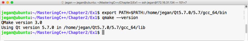
In case the qmake command isn't recognized, make sure you export the bin path of the Qt installation folder, as shown in the preceding screenshot. Additionally, creating a soft link might be useful too. The command for this is as follows:
sudo ln -s /home/jegan/Qt5.7.0/5.7/gcc_64/bin/qmake /usr/bin/qmake
The path where Qt is installed on your system might vary from mine, so please substitute the Qt path accordingly.
Qt Core is one of the modules supported by Qt. This module has loads of useful classes, such as QObject, QCoreApplication, QDebug, and so on. Almost every Qt application will require this module, hence they are linked implicitly by the Qt Framework. Every Qt class inherits from QObject, and the QObject class offers event handling support to Qt applications. QObject is the critical piece that supports the event handling mechanism; interestingly, even console-based applications can support event handling in Qt.
If you get a similar output to that shown in Figure 5.1, you are all set to get your hands dirty. Let's write our first Qt application, as shown in the following screenshot:
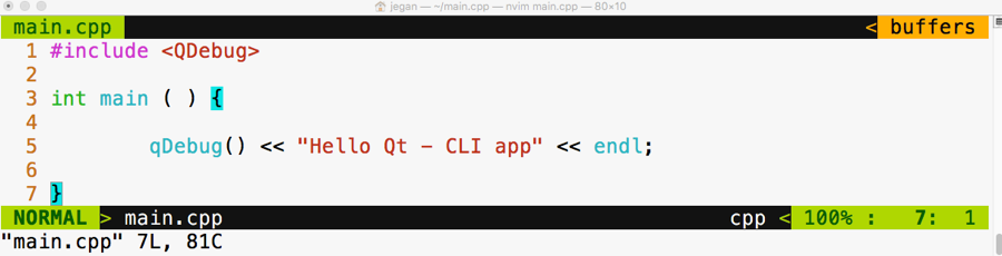
In the first line, we have included the QDebug header from the QtCore module. If you observe closely, the qDebug() function resembles the C++ cout ostream operator. The qDebug() function is going to be your good friend in the Qt world while you are debugging your code. The QDebug class has overloaded the C++ ostream operator in order to add support for Qt data types that aren't supported by the C++ compiler.
In old school fashion, I'm kind of obsessed with the Terminal to achieve pretty much anything while coding as opposed to using some fancy Integrated Development Environments (IDEs). You may either love or hate this approach, which is quite natural. The good part is there is nothing going to stand between you and Qt/C++ as you are going to use plain and simple yet powerful text editors, such as Vim, Emacs, Sublime Text, Atom, Brackets, or Neovim, so you will learn almost all the essentials of how Qt projects and qmake work; IDEs make your life easy, but they hide a lot of the essential stuff that every serious developer must know. So it's a trade-off. I leave it to you to decide whether to use your favorite plain text editor or Qt Creator IDE or any other fancy IDE. I'm going to stick with the refactored Vim editor called Neovim, which looks really cool. Figure 5.2 will give you an idea of the Neovim editor's look and feel.
Let's get back to business. Let's see how to compile this code in the command line the geeky way. Well, before that, you may want to know about the qmake tool. It is a proprietary make utility of Qt. The qmake utility is nothing more than a make tool, but it is aware of Qt-specific stuff so it knows about moc, signals, slots, and so on, which a typical make utility will be unaware of.
The following command should help you create a .pro file. The name of the .pro file will be decided by the qmake utility, based on the project folder name. The .pro file is the way the Qt Creator IDE combines related files as a single project. Since we aren't going to use Qt Creator, we will use the .pro file to create Makefile in order to compile our Qt project just like a plain C++ project.
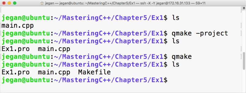
When you issue the qmake -project command, qmake will scan through the current folder and all the subfolders under the current folder and include the headers and source files in Ex1.pro. By the way, the .pro file is a plain text file that can be opened using any text editor, as shown in Figure 5.4:
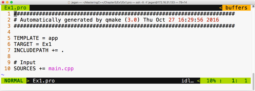
Now it's time to create Makefile taking Ex1.pro as an input file. As the Ex1.pro file is present in the current directory, we don't have to explicitly supply Ex1.pro as an input file to autogenerate Makefile. The idea is that once we have a .pro file, all we would need to do is generate Makefile from the .pro file issuing command: qmake. This will do all the magic of creating a full-blown Makefile for your project that you can use to build your project with the make utility, as shown in the following screenshot:
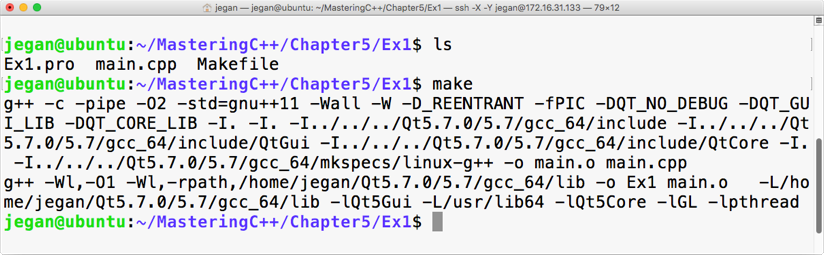
This is the point we have been waiting for, right? Yes, let's execute our first Qt Hello World program, as shown in the following screenshot:
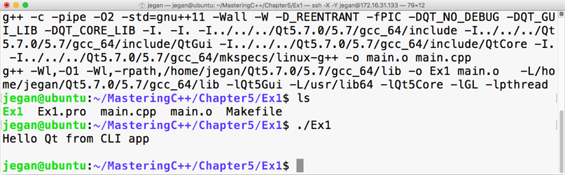
Congratulations! You have completed your first Qt application. In this exercise, you learned how to set up and configure Qt in Ubuntu and how to write a simple Qt console application and then build and run it. The best part is you learned all of this from the command line.
Qt Widgets is an interesting module that supports quite a lot of widgets, such as buttons, labels, edit, combo, list, dialog, and so on. QWidget is the base class of all of the widgets, while QObject is the base class of pretty much every Qt class. While many programming languages refer to as UI controls, Qt refers to them as widgets. Though Qt works on many platforms, its home remains Linux; widgets are common in the Linux world.
Our first console application is really cool, isn't it? Let's continue exploring further. This time, let's write a simple GUI-based Hello World program. The procedure will remain almost the same, except for some minor changes in main.cpp. Refer to the following for the complete code:
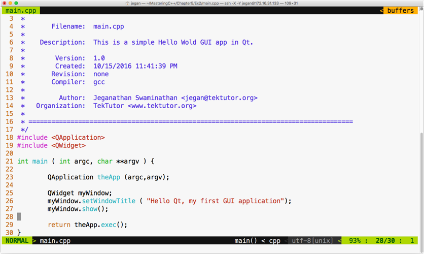
Wait a minute. Let me explain the need for QApplication in line number 23 and line number 29. Every Qt GUI application must have exactly one instance of the QApplication instance. QApplication provides support for command-line switches for our application, hence the need to supply the argument count (argc) and the argument value (argv). GUI-based applications are event-driven, so they must respond to events or, to be precise, signals in the Qt world. In line number 29, the exec function starts the event loop, which ensures the application waits for user interactions until the user closes the window. The idea is that all the user events will be received by the QApplication instance in an event queue, which will then be notified to its Child widgets. The event queue ensures all the events deposited in the queue are handled in the same sequence that they occur, that is, first in, first out (FIFO).
In case you are curious to check what would happen if you comment line 29, the application will still compile and run but you may not see any window. The reason being the main thread or the main function creates an instance of QWidget in line number 25, which is the window that we see when we launch the application.
In line number 27, the window instance is displayed, but in the absence of line number 29, the main function will terminate the application immediately without giving a chance for you to check your first Qt GUI application. It's worth trying, so go ahead and see what happens with and without line number 29.
Let's generate Makefile, as shown in the following screenshot:
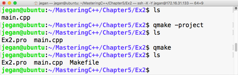
Now let's try to compile our project with the make utility, as shown in the following screenshot:
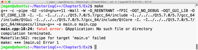
Interesting, right? Our brand new Qt GUI program fails to compile. Did you notice the fatal error? No big deal; let's understand why this happened. The reason is that we have not yet linked the Qt Widgets module, as the QApplication class is part of the Qt Widgets module. In that case, you may wonder how your first Hello World program compiled without any issue. In our first program, the QDebug class was part of the QtCore module that got linked implicitly, whereas other modules had to be linked explicitly. Let's see how to get this done:
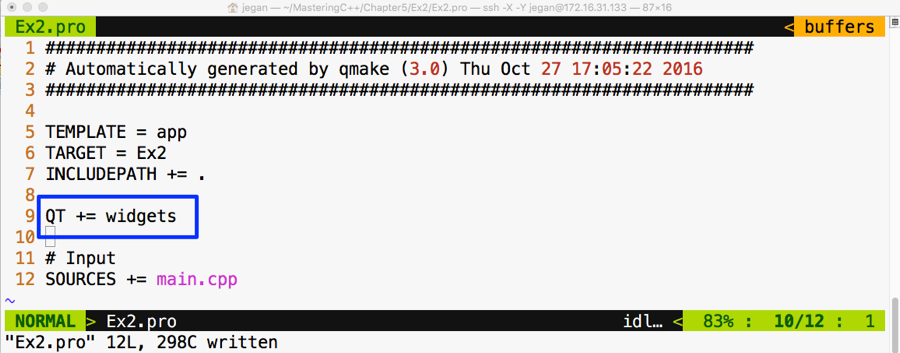
We need to add QT += widgets to the Ex2.pro file so that the qmake utility understands that it needs to link Qt Widgets's shared object (the .so file) in Linux, also known as the Dynamic Link Library (the .dll file) in Windows, while creating the final executable. Once this is taken care of, we must qmake so that Makefile could reflect the new change in our Ex2.pro file, as demonstrated in the following screenshot:
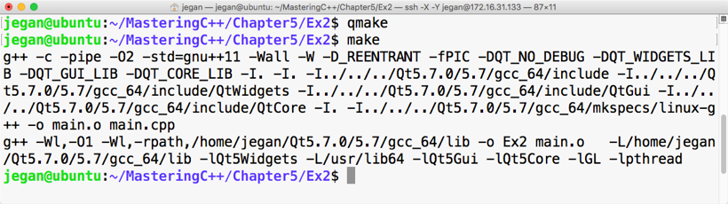
Cool. Let's check our first GUI-based Qt app now. In my system, the application output looks as shown in Figure 5.12; you should get a similar output as well if all goes well at your end:
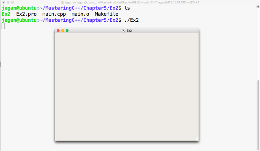
It would be nice if we set the title of our window as Hello Qt, right? Let's do this right away:
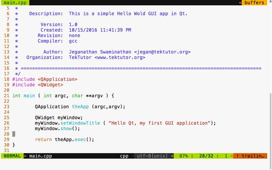
Add the code presented at line number 26 to ensure you build your project with the make utility before you test your new change:
Qt is cross-platform application framework, hence it supports concepts such as layouts for developing applications that look consistent in all platforms, irrespective of the different screen resolutions. When we develop GUI/HMI-based Qt applications, an application developed in one system shouldn't appear different on another system with a different screen size and resolution. This is achieved in the Qt Framework via layouts. Layouts come in different flavors. This helps a developer design a professional-looking HMI/GUI by organizing various widgets within a window or dialog. Layouts differ in the way they arrange their child widgets. While one arranges its child widgets in a horizontal fashion, another will arrange them in a vertical or grid fashion. When a window or dialog gets resized, the layouts resize their child widgets so they don't get truncated or go out of focus.
Let's write a Qt application that has a couple of buttons in the dialog. Qt supports a variety of useful layout managers that act as an invisible canvas where many QWidgets can be arranged before they are attached to a window or dialog. Each dialog or window can have only one layout. Every widget can be added to only one layout; however, many layouts can be combined to design a professional UI.
Let's start writing the code now. In this project, we are going to write code in a modular fashion, hence we are going to create three files with the names MyDlg.h, MyDlg.cpp, and main.cpp.
The game plan is as follows:
It is important that we follow clean code practices so that our code is easy to understand and can be maintained by anyone. As we are going to follow industry best practices, let's declare the dialog in a header file called MyDlg.h, define the dialog in the source file called MyDlg.cpp, and use MyDlg.cpp in main.cpp that has the main function. Every time MyDlg.cpp requires a header file, let's make it a practice to include all the headers only in MyDlg.h; with this, the only header we will see in MyDlg.cpp is MyDlg.h.
By the way, did I tell you Qt follows the camel casing coding convention? Yes, I did mention it right now. By now, you will have observed that all Qt classes start with the letter Q because Qt inventors loved the letter "Q" in Emacs and they were so obsessed with that font type that they decided to use the letter Q everywhere in Qt.
One last suggestion. Wouldn't it be easy for others to locate the dialog class if the name of the file and the name of the class were similar? I can hear you say yes. All set! Let's start coding our Qt application. First, refer to the following screenshot:
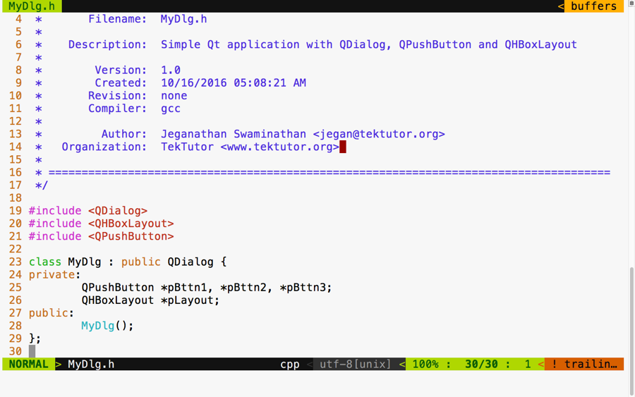
In the preceding screenshot, we declared a class with the name MyDlg. It has one layout, three buttons, and a constructor. Now refer to this screenshot:
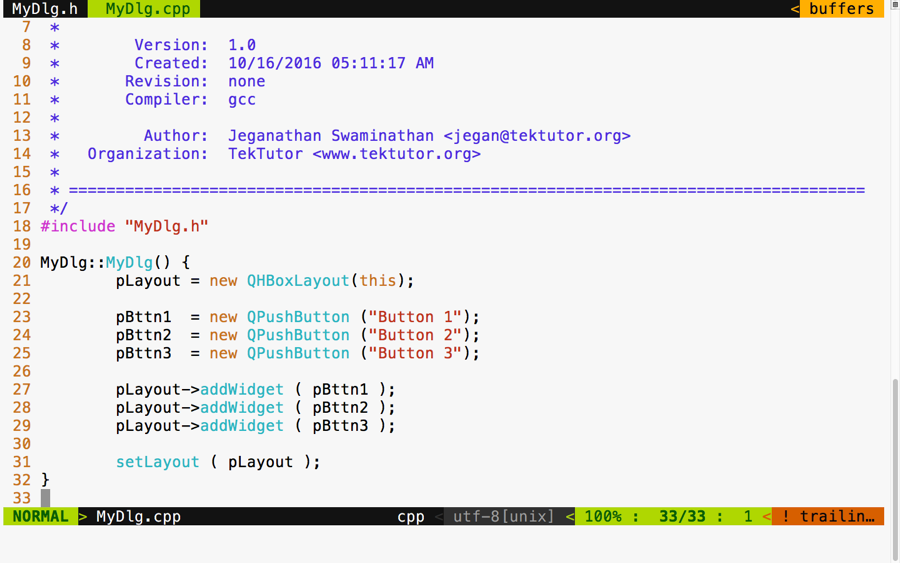
As you can see in the preceding screenshot, we defined the MyDlg constructor and instantiated the layout and the three buttons. In lines 27 through 29, we added three buttons to the layout. In line number 31, we associated the layout to our dialog. That's all it takes. In the following screenshot, we defined our main function, which creates an instance of QApplication:
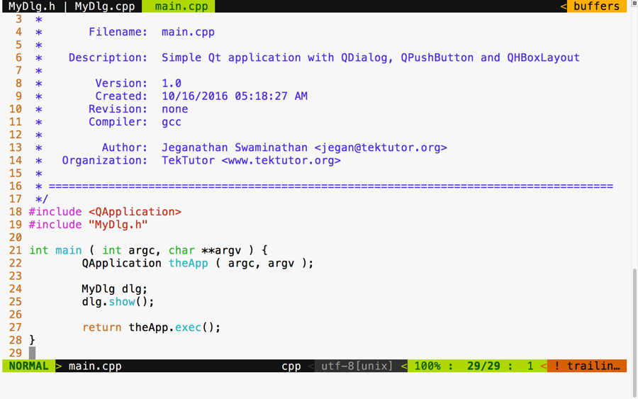
We followed this up by creating our custom dialog instance and displaying the dialog. Finally, at line 27, we started the event loop so that MyDlg could respond to user interactions. Refer to the following screenshot:
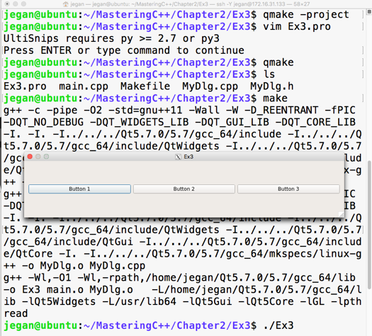
The preceding screenshot demonstrates the build and execution procedures, and there is our cute application. Actually, you can try playing with the dialog to understand the horizontal layout better. First, stretch the dialog horizontally and notice all the buttons' width increase; then, see whether you can reduce the dialog's width to notice all the buttons' width decrease. That's the job of any layout manager. A layout manager arranges widgets and retrieves the size of the window and divides the height and width equally among all its child widgets. Layout managers keep notifying all their child widgets about any resize events. However, it is up to the respective child widget to decide whether they want to resize themselves or ignore the layout resize signals.
To check this behavior, try stretching out the dialog vertically. As you increase the height of the dialog, the dialog's height should increase, but the buttons will not increase their height. This is because every Qt Widget has its own preferred size policy; as per their size policy, they may respond or ignore certain layout resize signals.
If you want the buttons to stretch vertically as well, QPushButton offers a way to get this done. In fact, QPushButton extends from QWidget just like any other widget. The setSizePolicy() method comes to QPushButton from its base class, that is, QWidget:
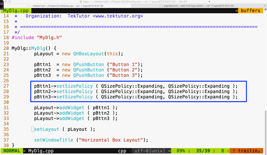
Did you notice line number 37? Yes, I have set the window title within the constructor of MyDlg to keep our main function compact and clean.
Make sure you have built your project using the make utility before launching your application:
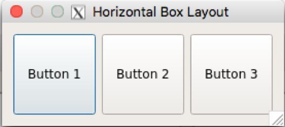
In the highlighted section, we have overridden the default size policy of all the buttons. In line number 27, the first parameter QSizePolicy::Expanding refers to the horizontal policy and the second parameter refers to the vertical policy. To find other possible values of QSizePolicy, refer to the assistant that comes in handy with the Qt API reference, as shown in the following screenshot:
In the previous section, you learned how to use a horizontal box layout. In this section, you will see how to use a vertical box layout in your application.
As a matter of fact, the horizontal and vertical box layouts vary only in terms of how they arrange the widgets. For instance, the horizontal box layout will arrange its child widgets in a horizontal fashion from left to right, whereas the vertical box layout will arrange its child widgets in a vertical fashion from top to bottom.
You can copy the source code from the previous section, as the changes are minor in nature. Once you have copied the code, your project directory should look as follows:
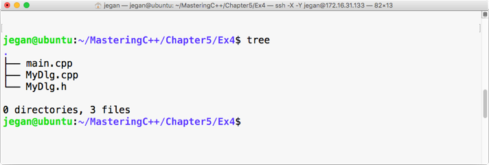
Let me demonstrate the changes starting from the MyDlg.h header file, as follows:
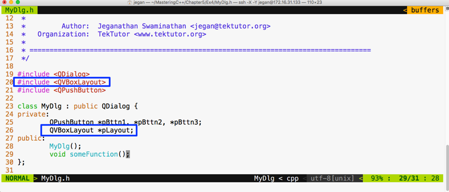
I have replaced QHBoxLayout with QVBoxLayout; that is all. Yes, let's proceed with file changes related to MyDlg.cpp:
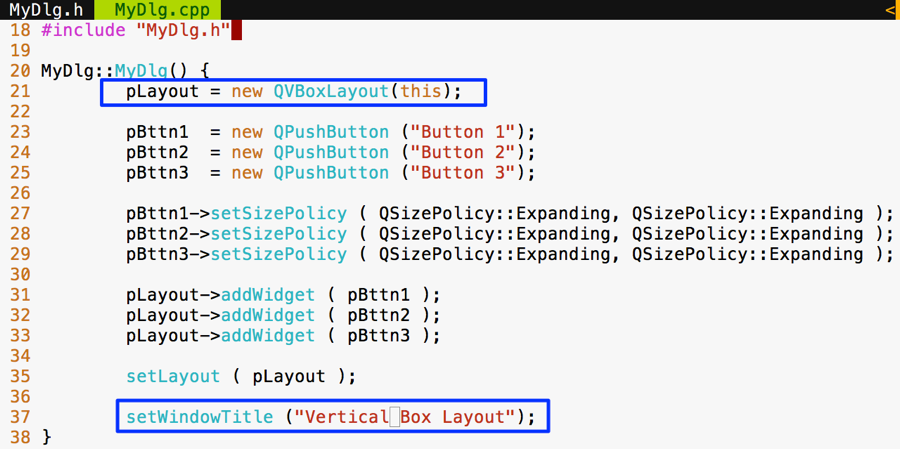
There are no changes to be done in main.cpp; however, I have shown main.cpp for your reference, as follows:
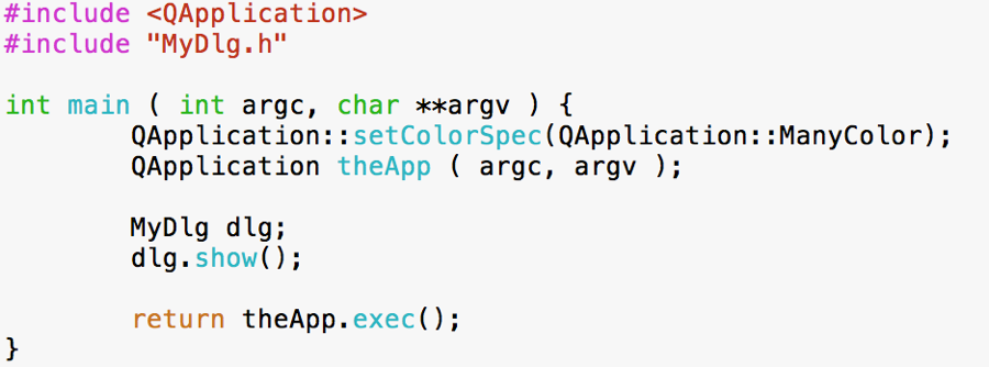
Now all we need to do is autogenerate Makefile and then make and run the program as follows:
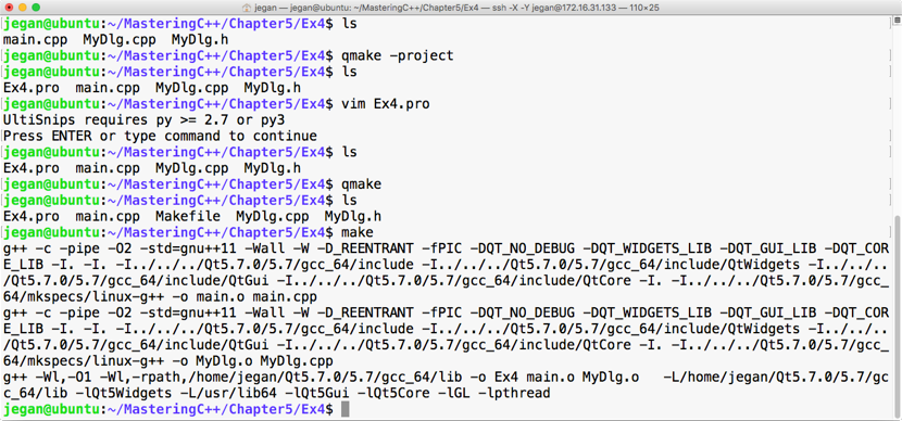
Let's execute our brand new program and check the output. The following output demonstrates that QVBoxLayout arranges the widgets in a vertical top to bottom fashion. When the window is stretched, all the buttons' width will increase/decrease depending on whether the window is stretched out or stretched in:
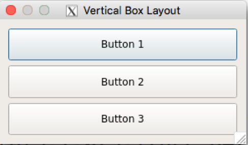
In the previous sections, you learned how to make use of QHBoxLayout and QVBoxLayout. Actually, these two classes are the convenience classes for QBoxLayout. In the case of QHBoxLayout, the QHBoxLayout class has subclassed QBoxLayout and configured QBoxLayout::Direction to QBoxLayout::LeftToRight, whereas the QVBoxLayout class has subclassed QBoxLayout and configured QBoxLayout::Direction to QBoxLayout::TopToBottom.
Apart from these values, QBoxLayout::Direction supports various other values, as follows:
Let's write a simple program using QBoxLayout with five buttons.
Let's start with the MyDlg.h header file. I have declared five button pointers in the MyDlg class and a QBoxLayout pointer:
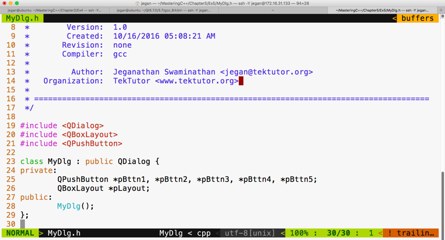
Let's take a look at our MyDlg.cpp source file. If you notice line number 21 in the following screenshot, the QBoxLayout constructor takes two arguments. The first argument is the direction in which you wish to arrange the widgets and the second argument is an optional argument that expects the parent address of the layout instance.
As you may have guessed, the this pointer refers to the MyDlg instance pointer, which happens to be the parent of the layout.
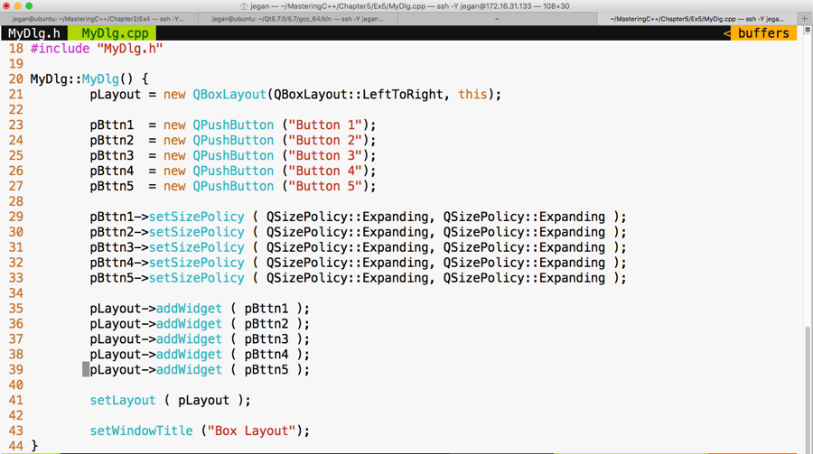
Again, as you may have guessed, the main.cpp file isn't going to change from our past exercises, as shown in the following screenshot:
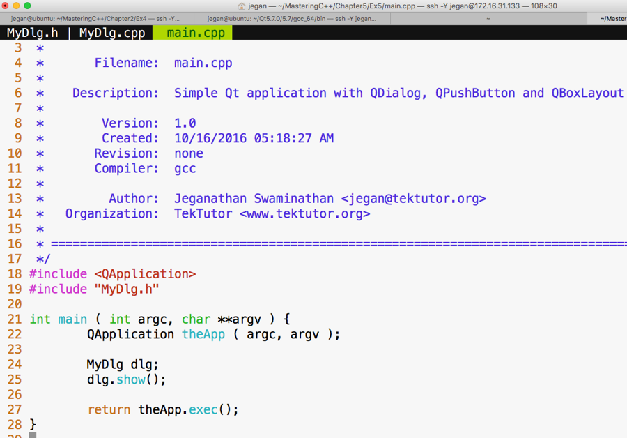
Let's compile and run our program, as follows:
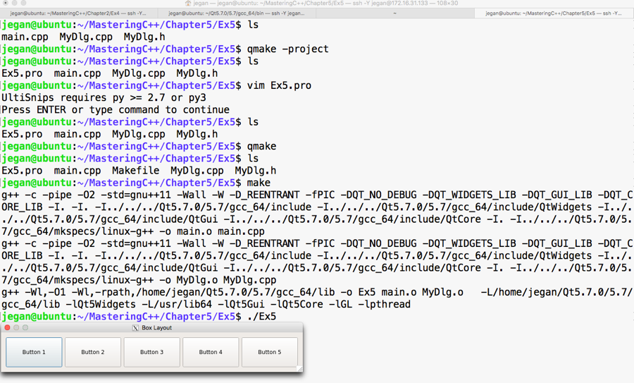
If you notice the output, it looks like a horizontal box layout output, right? Exactly, because we have set the direction to QBoxLayout::LeftToRight. If you modify the direction to, say, QBoxLayout::RightToLeft, then Button 1 would appear on the right-hand side, Button 2 would appear on the left-hand side of Button 1, and so on. Hence, the output would look as shown in the following screenshot:
If the direction is set to QBoxLayout::RightToLeft, you'll see the following output:
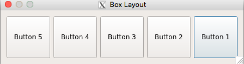
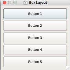
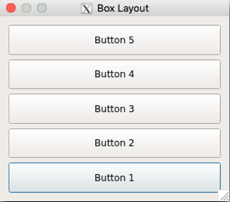
In all the preceding scenarios, the buttons are added to the layout exactly in the same sequence, starting from Button 1 through Button 5, respectively. However, depending on the direction chosen in the QBoxLayout constructor, the box layout will arrange the buttons, hence the difference in the output.
A grid layout allows us to arrange widgets in a tabular fashion. It is quite easy, just like a box layout. All we need to do is indicate the row and column where each widget must be added to the layout. As the row and column index starts from a zero-based index, the value of row 0 indicates the first row and the value of column 0 indicates the first column. Enough of theory; let's start writing some code.
Let's declare 10 buttons and add them in two rows and five columns. Other than the specific QGridLayout differences, the rest of the stuff will remain the same as the previous exercises, so go ahead and create MyDlg.h, MyDl.cpp, and main.cpp if you have understood the concepts discussed so far.
Let me present the MyDlg.h source code in the following screenshot:
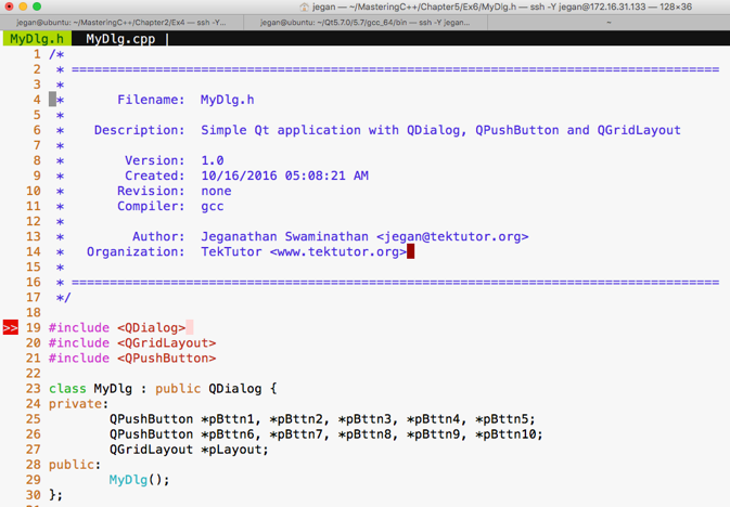
The following is the code snippet of MyDlg.cpp:
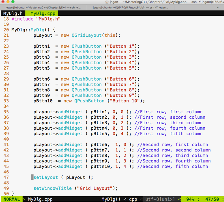
The main.cpp source file content will remain the same as our previous exercises; hence, I have skipped the main.cpp code snippet. As you are familiar with the build process, I have skipped it too. If you have forgotten about this, just check the previous sections to understand the build procedure.
If you have typed the code correctly, you should get the following output:
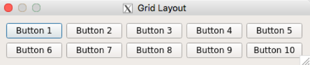
Actually, the grid layout has more stuff to offer. Let's explore how we can make a button span across multiple cells. I guarantee what you are about to see is going to be more interesting.
I'm going to modify MyDlg.h and MyDlg.cpp and keep main.cpp the same as the previous exercises:
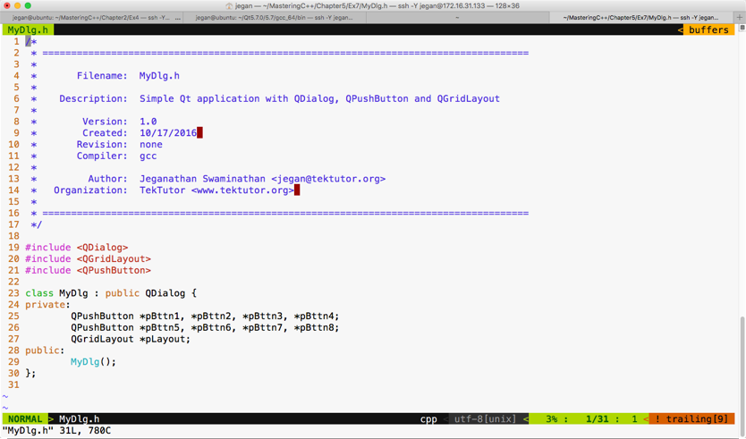
Here goes our MyDlg.cpp:
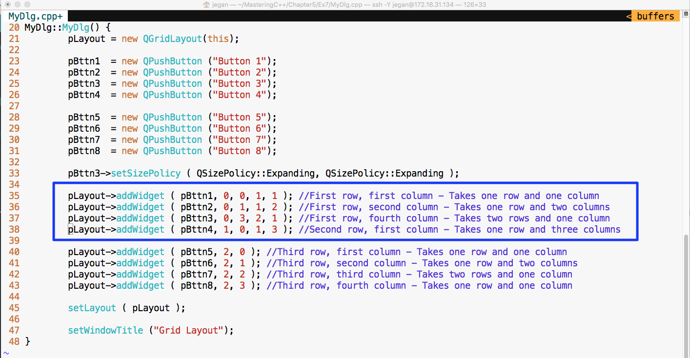
Notice the lines 35 through 38. Let's discuss the addWidget() function in detail now.
In line number 35, the pLayout->addWidget ( pBttn1, 0, 0, 1, 1 ) code does the following things:
In line number 36, the pLayout->addWidget ( pBttn2, 0, 1, 1, 2 ) code does the following:
In line number 37, the pLayout->addWidget ( pBttn3, 0, 3, 2, 1 ) code does the following:
In line number 38, the pLayout->addWidget ( pBttn4, 1, 0, 1, 3 ) code does the following:
Check out the output of the program:
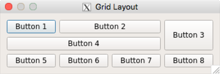
Signals and slots are an integral part of the Qt Framework. So far, we have written some simple but interesting Qt applications, but we haven't handled events. Now it's time to understand how to support events in our application.
Let's write a simple application with just one button. When the button is clicked, check whether we can print something on the console.
The MyDlg.h header demonstrates how the MyDlg class shall be declared:
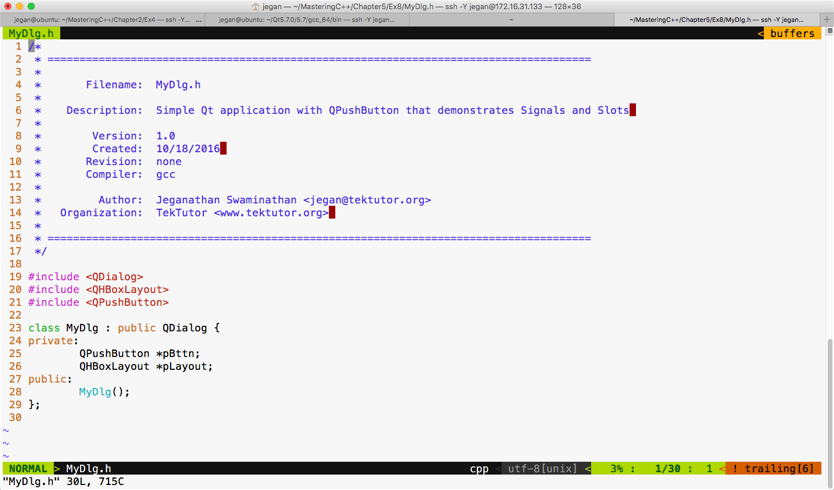
The following screenshot demonstrates how the MyDlg constructor shall be defined to add a single button to our dialog window:
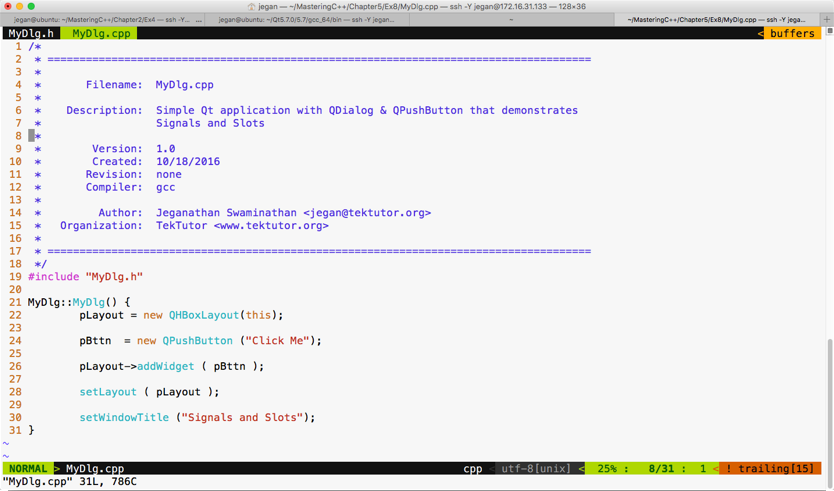
The main.cpp looks as follows:
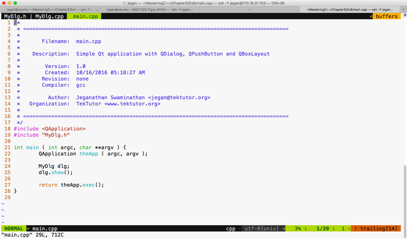
Let's build and run our program and later add support for signals and slots. If you have followed the instructions correctly, your output should resemble the following screenshot:
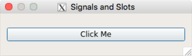
If you click on the button, you will notice that nothing happens, as we are yet to add support for signals and slots in our application. Okay, it's time to reveal the secret instruction that will help you make the button respond to a button-click signal. Hold on, it's time for some more information. Don't worry, it's related to Qt.
Qt signals are nothing but events, and slot functions are event handler functions. Interestingly, both signals and slots are normal C++ functions; only when they are marked as signals or slots, will the Qt Framework understand their purpose and provide the necessary boilerplate code.
Every widget in Qt supports one or more signal and may also optionally support one or more slot. So let's explore which signals QPushButton supports before we write any further code.
Let's make use of the Qt assistant for API reference:
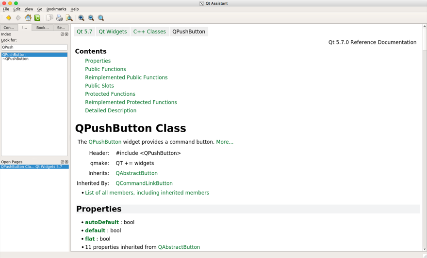
If you observe the preceding screenshot, it has a Contents section that seems to cover Public Slots, but we don't see any signals listed there. That's a lot of information. If the Contents section doesn't list out signals, QPushButton wouldn't support signals directly. However, maybe its base class, that is, QAbstractButton, would support some signals. The QPushButton class section gives loads of useful information, such as the header filename, which Qt module must be linked to the application--that is, qmake entries that must be added to .pro--and so on. It also mentions the base class of QPushButton. If you scroll down further, your Qt assistant window should look like this:
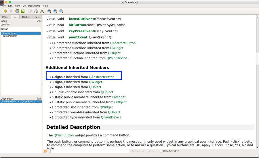
If you observe the highlighted section under Additional Inherited Members, apparently the Qt assistant implies that QPushButton has inherited four signals from QAbstractButton. So we need to explore the signals supported by QAbstractButton in order to support the signals in QPushButton.
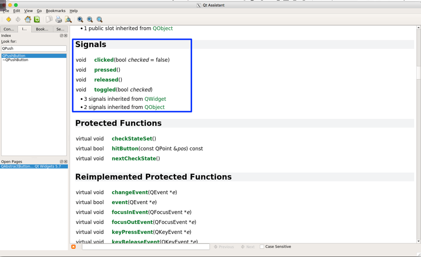
With the help of the Qt assistant, as shown in the preceding screenshot, it is evident that the QAbstractButton class supports four signals that are also available for QPushButton, as QPushButton is a child class of QAbstractButton. So let's use the clicked() signal in this exercise.
We need to make some minor changes in MyDlg.h and MyDlg.cpp in order to use the clicked() signal. Hence, I have presented these two files with changes highlighted in the following screenshot:
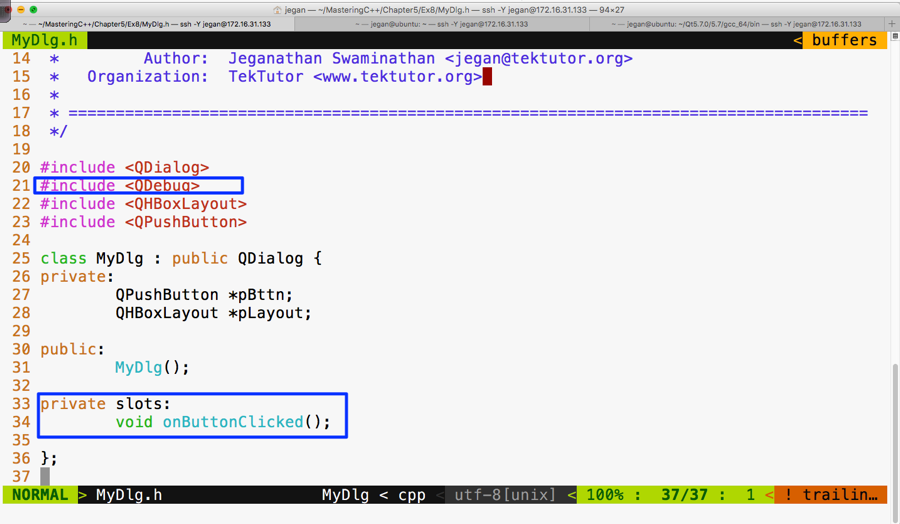
As you are aware, the QDebug class is used for debugging purposes. It offers functionalities to Qt applications that are similar to cout, but they aren't really required for signals and slots. We are using them here just for debugging purposes. In Figure 5.48, line number 34, void MyDlg::onButtonClicked() is our slot function that we are intending to use as an event handler function that must be invoked in response to the button click.
The following screenshot should give you an idea of what changes you will have to perform in MyDlg.cpp for signal and slot support:
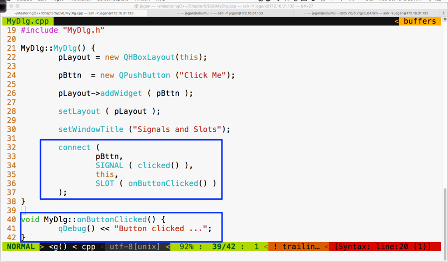
If you observe line 40 through 42 in the preceding screenshot, the MyDlg::onButtonClicked() method is a slot function that must be invoked whenever the button is clicked. But unless the button's clicked() signal is mapped to the MyDlg::onButtonClicked() slot, the Qt Framework wouldn't know that it must invoke MyDlg::onButtonClicked() when the button is clicked. Hence, in line numbers 32 through 37, we have connected the button signal clicked() with the MyDlg instance's onButtonClicked() slot function. The connect function is inherited by MyDlg from QDialog. This, in turn, has inherited the function from its ultimate base class, called QObject.
The mantra is that every class that would like to participate in signal and slot communication must be either QObject or its subclass. QObject offers quite a good amount of signal and slot support, and QObject is part of the QtCore module. What's amazing is that the Qt Framework has made signal and slot available to even command-line applications. This is the reason signals and slots support is built into the ultimate base class QObject, which is part of the QtCore module.
Okay, let's build and run our program and see whether the signals work in our application:
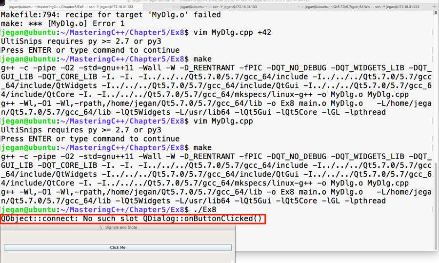
Interestingly, we don't get a compilation error, but when we click on the button, the highlighted warning message appears automatically. This is a hint from the Qt Framework that we have missed out on an important procedure that is mandatory to make signals and slots work.
Let's recollect the procedure we followed to autogenerate Makefile in our headers and source files:
In step 1, the qmake utility scans through all our custom header files and checks whether they need signal and slot support. Any header file that has the Q_OBJECT macro hints the qmake utility that it needs signal and slot support. Hence we must use the Q_OBJECT macro in our MyDlg.h header file:
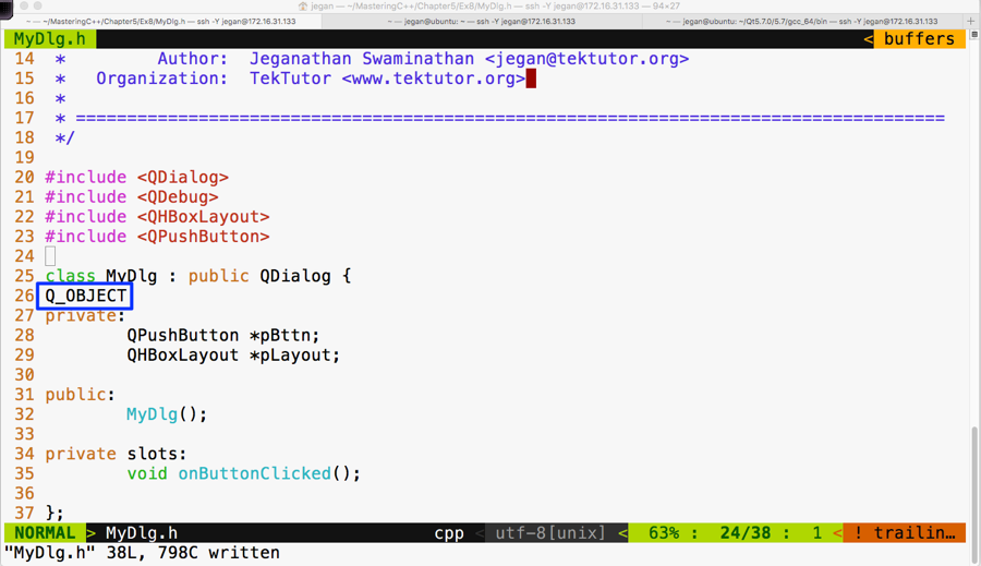
Once the recommended changes are done in the header file, we need to ensure that the qmake command is issued. Now the qmake utility will open the Ex8.pro file to get our project headers and source files. When qmake parses MyDlg.h and finds the Q_OBJECT macro, it will learn that our MyDlg.h requires signals and slots, then it will ensure that the moc compiler is invoked on MyDlg.h so that the boilerplate code can be autogenerated in a file called moc_MyDlg.cpp. This will then go ahead and add the necessary rules to Makefile so that the autogenerated moc_MyDlg.cpp file gets built along with the other source files.
Now that you know the secrets of Qt signals and slots, go ahead and try out this procedure and check whether your button click prints the Button clicked ... message. I have gone ahead and built our project with the changes recommended. In the following screenshot, I have highlighted the interesting stuff that goes on behind the scenes; these are some of the advantages one would get when working in the command line versus using fancy IDEs:
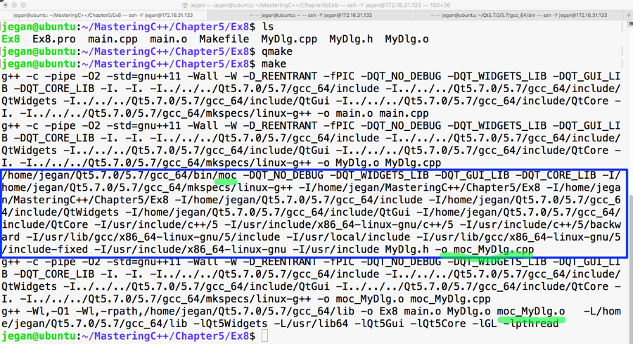
Now it's time that we test the output of our cool and simple application that supports signals and slots. The output is presented in the following screenshot:
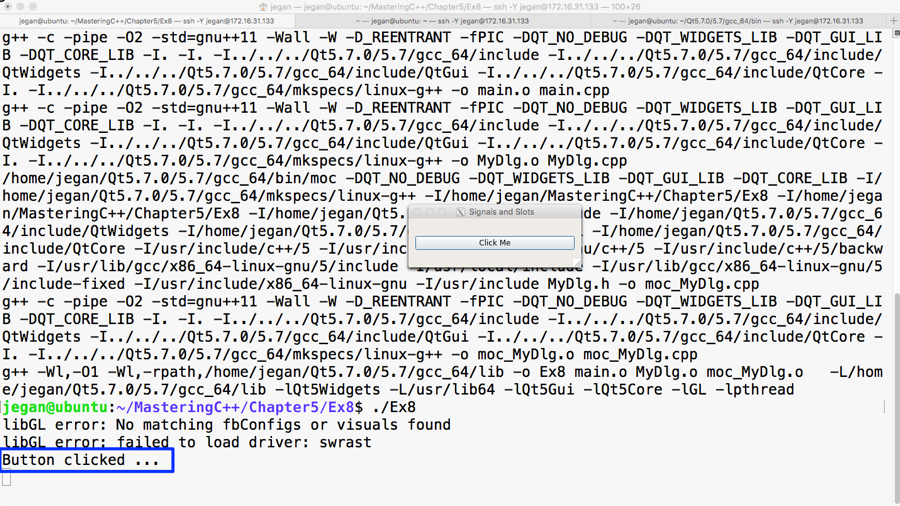
Congratulations! You can pat your back. You have learned enough to do cool stuff in Qt.
As you have learned about signals and slots, in this section, let's explore how to use a stacked layout in an application that has multiple windows; each window could be either a QWidget or QDialog. Each page may have its own child widgets. The application we are about to develop will demonstrate the use of a stacked layout and how to navigate from one window to the other within the stacked layout.
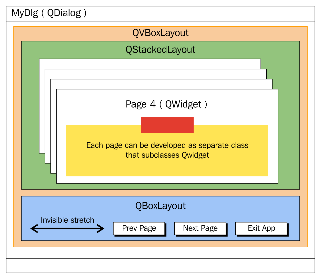
This application is going to require a decent amount of code, hence it is important that we ensure our code is structured carefully so that it meets both the structural and functional quality, avoiding code smells as much as possible.
Let's create four widgets/windows that could be stacked up in a stacked layout, where each page could be developed as a separate class split across two files: HBoxDlg.h and HBoxDlg.cpp and so on.
Let's start with HBoxDlg.h. As you are familiar with layouts, in this exercise, we are going to create each dialog with one layout so that while navigating between the subwindows, you can differentiate between the pages. Otherwise, there will be no connection between the stacked layout and other layouts as such.
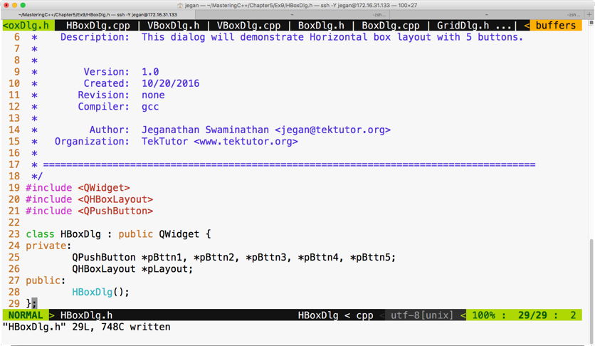
The following code snippet is from the HBoxDlg.cpp file:
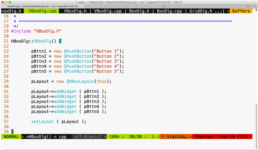
Similarly, let's write VBoxDlg.h as follows:
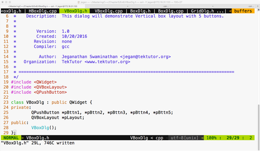
Let's create the third dialog BoxDlg.h with a box layout, as follows:
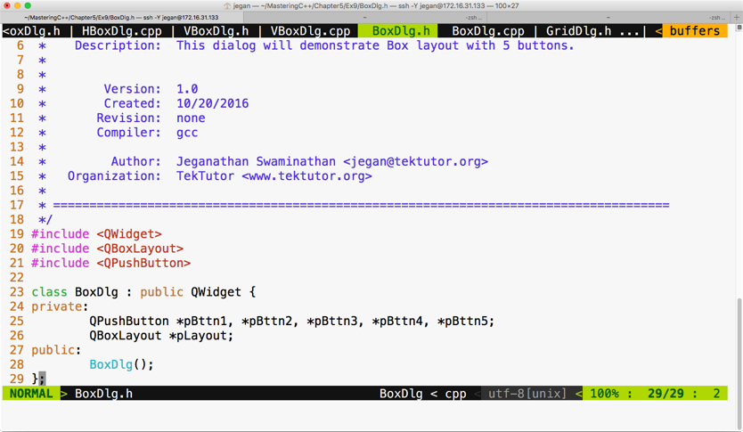
The respective BoxDlg.cpp source file will look as follows:
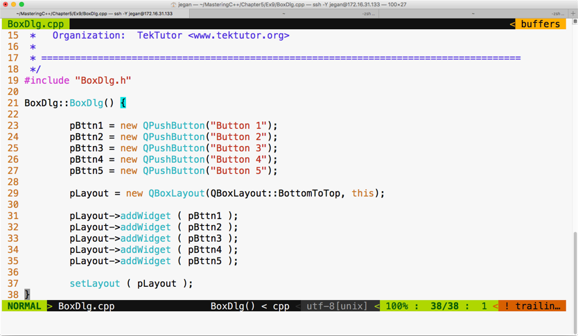
The fourth dialog that we would like to stack up is GridDlg, so let's see how GridDlg.h can be written, which is illustrated in the following screenshot:

The respective GridDlg.cpp will look like this:
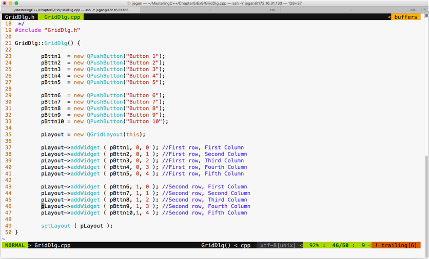
Cool, we are done with creating four widgets that can be stacked up in MainDlg. MainDlg is the one that's going to use QStackedLayout, so the crux of this exercise is understanding how a stacked layout works.
Let's see how MainDlg.h shall be written:
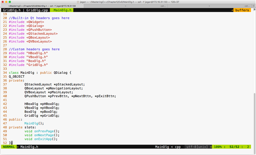
In MainDlg, we have declared three slot functions, one for each button, in order to support the navigation logic among the four windows. A stacked layout is similar to a tabbed widget, except that a tabbed widget will provide its own visual way to switch between the tabs, whereas in the case of a stacked layout, it is up to us to provide the switching logic.
The MainDlg.cpp will look like this:
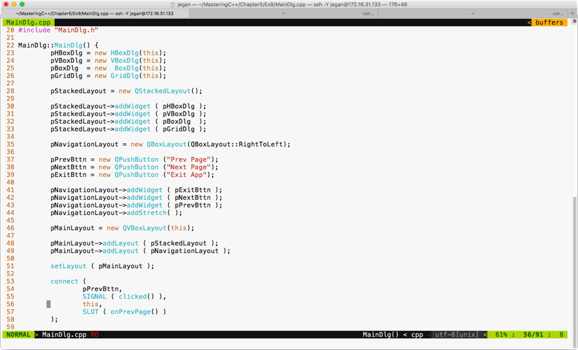
You can choose a box layout to hold the three buttons, as we prefer buttons aligned to the right. However, in order to ensure that extra spaces are consumed by some invisible glue, we have added a stretch item at line number 44.
Between lines 30 through 33, we have added all the four subwindows in a stacked layout so that windows can be made visible one at a time. The HBox dialog is added at index 0, the VBox dialog is added at index 1, and so on.
Lines 53 through 58 demonstrate how the previous button's clicked signal is wired with its corresponding MainDlg::onPrevPage() slot function. Similar connections must be configured for next and exit buttons:
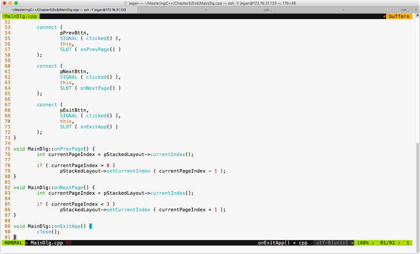
The if condition in line 78 ensures that the switching logic happens only if we are in the second or later subwindows. As the horizontal dialog is at index 0, we can't navigate to the previous window in cases where the current window happens to be a horizontal dialog. A similar validation is in place for switching to the next subwindow in line 85.
The stacked layout supports the setCurrentIndex() method to switch to a particular index position; alternatively, you could try the setCurrentWidget() method as well if it works better in your scenario.
The main.cpp looks short and simple, as follows:
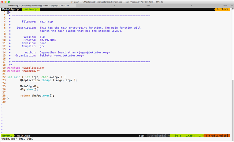
The best part of our main function is that irrespective of the complexity of the application logic, the main function doesn't have any business logic. This makes our code clean and easily maintainable.
In this section, let's explore how to write a simple math application. As part of this exercise, we will use QLineEdit and QLabel widgets and QFormLayout. We need to design a UI, as shown in the following screenshot:
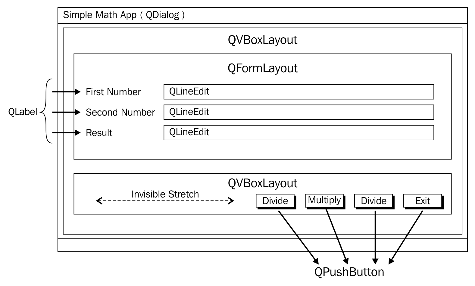
QLabel is a widget typically used for static text, and QLineEdit will allow a user to supply a single line input. As shown in the preceding screenshot, we will use QVBoxLayout as the main layout in order to arrange QFormLayout and QBoxLayout in a vertical fashion. QFormLayout comes in handy when you need to create a form where there will be a caption on the left-hand side followed by some widget on its right. QGridLayout might also do the job, but QFormLayout is easy to use in such scenarios.
In this exercise, we will create three files, namely MyDlg.h, MyDlg.cpp, and main.cpp. Let's start with the MyDlg.h source code and then move on to other files:
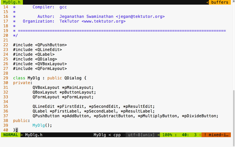
In the preceding figure, three layouts are declared. The vertical box layout is used as the main layout, while the box layout is used to arrange the buttons in the right-aligned fashion. The form layout is used to add the labels, that is, line edit widgets. This exercise will also help you understand how one can combine multiple layouts to design a professional HMI.
Qt doesn't have any documented restriction in the number of layouts that can be combined in a single window. However, when possible, it is a good idea to consider designing an HMI with a minimal number of layouts if you are striving to develop a small memory footprint application. Otherwise, there is certainly no harm in using multiple layouts in your application.
In the following screenshot, you will get an idea of how the MyDlg.cpp source file shall be implemented. In the MyDlg constructor, all the buttons are instantiated and laid out in the box layout for right alignment. The form layout is used to hold the QLineEdit widgets and their corresponding QLabel widgets in a grid-like fashion. QLineEdit widgets typically help supply a single line input; in this particular exercise, they help us supply a number input that must be added, subtracted, and so on, depending on the user's choice.
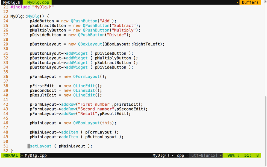
The best part of our main.cpp source file is that it remains pretty much the same, irrespective of the complexity of our application. In this exercise, I would like to tell you a secret about MyDlg. Did you notice that the MyDlg constructor is instantiated in the stack as opposed to the heap? The idea is that when the main() function exits, the stack used by the main function gets unwinded, eventually freeing up all the stack variables present in the stack. When MyDlg gets freed up, it results in calling the MyDlg destructor. In the Qt Framework, every widget constructor takes an optional parent widget pointer, which is used by the topmost window destructor to free up its child widgets. Interestingly, Qt maintains a tree-like data structure to manage the memory of all its child widgets. So, if all goes well, the Qt Framework will take care of freeing up all its child widgets' memory locations "automagically".
This helps Qt developers focus on the application aspect, while the Qt Framework will take care of memory management.
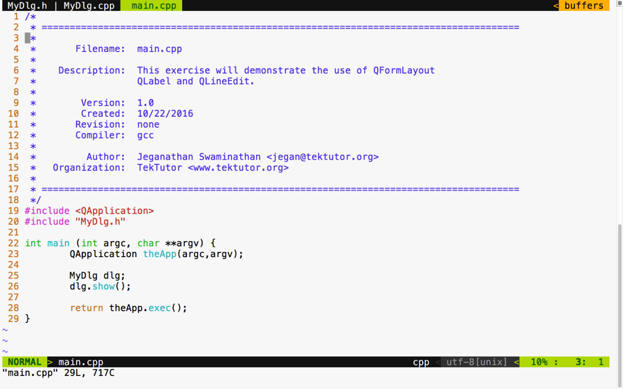
Aren't you excited to check the output of our new application? If you build and execute the application, then you are supposed to get an output similar to the following screenshot. Of course, we are yet to add signal and slot support, but it's a good idea to design the GUI to our satisfaction and then shift our focus to event handling:
If you observe closely, though the buttons are laid out on QBoxLayout in the right to left direction, the buttons aren't aligned to the right. The reason for this behavior is when the window is stretched out, the box layout seems to have divided and allocated the extra horizontal space available among all the buttons. So let's go ahead and throw in a stretch item to the leftmost position on the box layout such that the stretch will eat up all the extra spaces, leaving the buttons no room to expand. This will get us the right-aligned effect. After adding the stretch, the code will look as shown in the following screenshot:
Go ahead and check whether your output looks as shown in the following screenshot. Sometimes, as developers, we get excited to see the output in a rush and forget to compile our changes, so ensure the project is built again. If you don't see any change in output, no worries; just try to stretch out the window horizontally and you should see the right-aligned effect, as shown in the following screenshot:
Now since we have a decent-looking application, let's add signal and slot support to add the response to button clicks. Let's not rush and include the add and subtract functionalities for now. We will use some qDebug() print statements to check whether the signals and slots are connected properly and then gradually replace them with the actual functionalities.
If you remember the earlier signal and slot exercise, any Qt window that is interested in supporting signals and slots must be QObject and should include the Q_OBJECT macro in the MyDlg.h header file, as shown in the following screenshot:
In lines starting from 41 through 45, four slot methods are declared in the private section. Slot functions are regular C++ functions that could be invoked directly just like other C++ functions. However, in this scenario, the slot functions are intended to be invoked only with MyDlg. Hence they are declared as private functions, but they could be made public if you believe that others might find it useful to connect to your public slot.
Cool, if you have come this far, it says that you have understood the things discussed so far. Alright, let's go ahead and implement the definitions for the slot functions in MyDlg.cpp and then connect the clicked() button's signals with the respective slot functions:
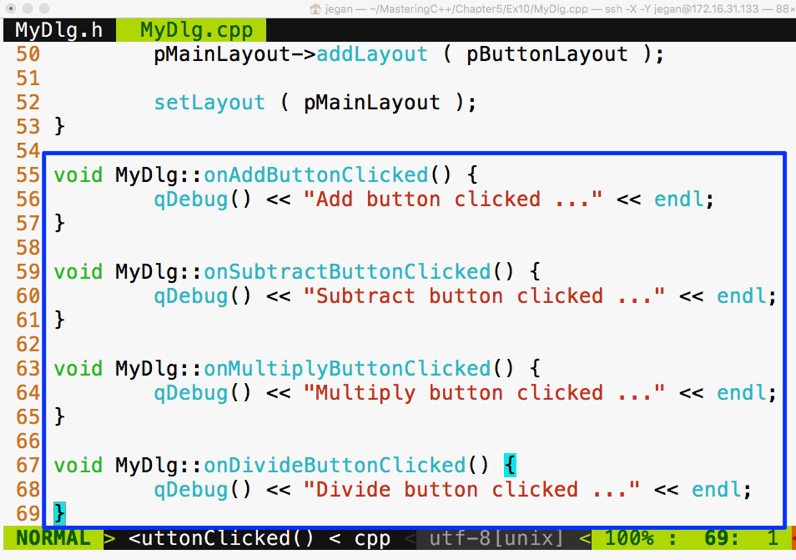
Now it's time to wire up the signals to their respective slots. As you may have guessed, we need to use the connect function in the MyDlg constructor, as shown in the following screenshot, to get the button clicks to the corresponding slots:
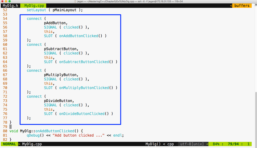
We are all set. Yes, it's showtime now. As we have taken care of most of the stuff, let's compile and check the output of our little Qt application:
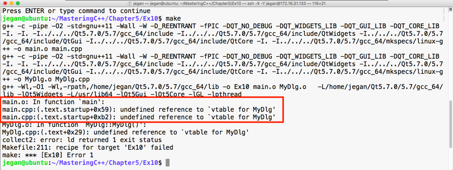
Oops! We got some linker error. The root cause of this issue is that we forgot to invoke qmake after enabling signal and slot support in our application. No worries, let's invoke qmake and make and run our application:
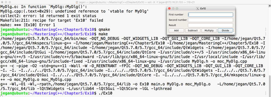
Great, we have fixed the issue. The make utility doesn't seem to make any noise this time and we are able to launch the application. Let's check whether the signals and slots are working as expected. For this, click on the Add button and see what happens:
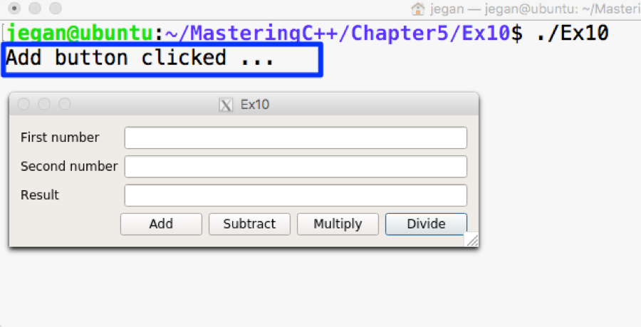
Wow! When we click on the Add button, the qDebug() console message confirms that the MyDlg::onAddButtonClicked() slot is invoked. If you are curious to check the slots of other buttons, go ahead and try clicking on the rest of the buttons.
Our application will be incomplete without business logic. So let's add business logic to the MyDlg::onAddButtonClicked() slot function to perform the addition and display the result. Once you learn how to integrate the added business logic, you can follow the same approach and implement the rest of the slot functions:
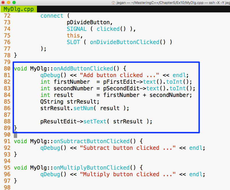
In the MyDlg::onAddButtonClicked() function, the business logic is integrated. In lines 82 and 83, we are trying to extract the values typed by the user in the QLineEdit widgets. The text() function in QLineEdit returns QString. The QString object provides toInt() that comes in handy to extract the integer value represented by QString. Once the values are added and stored in the result variable, we need to convert the result integer value back to QString, as shown in line number 86, so that the result can be fed into QLineEdit, as shown in line number 88.
Similarly, you can go ahead and integrate the business logic for other math operations. Once you have thoroughly tested the application, you can remove the qDebug() console's output. We added the qDebug() messages for debugging purposes, hence they can be cleaned up now.
In this chapter, you learned developing C++ GUI applications using Qt application framework. The key takeaway points are listed below.
In the next chapter, you will be learning multithread programming and IPC in C++.
This chapter will cover the following topics:
Let's deep dive into these TDD topics.
Test-driven development (TDD) is an extreme programming practice. In TDD, we start with a test case and incrementally write the production code that is required to make the test case succeed. The idea is that one should focus on one test case or scenario at a time and once the test case passes, they can then move on to the next scenario. In this process, if the new test case passes, we shouldn't modify the production code. In other words, in the process of developing a new feature or while fixing a bug, we can modify the production code only for two reasons: either to ensure the test case passes or to refactor the code. The primary focus of TDD is unit testing; however, it can be extended to integration and interaction testing to some extent.
The following figure demonstrates the TDD process visually:
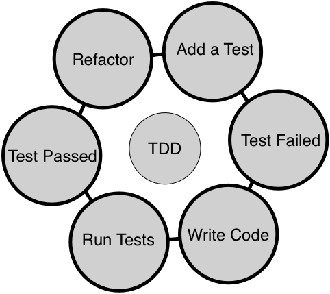
When TDD is followed religiously, one can achieve both functional and structural quality of the code. It is very crucial that you write the test case first before writing the production code as opposed to writing test cases at the end of the development phase. This makes quite a lot of difference. For instance, when a developer writes unit test cases at the end of development, it is very unlikely that the test cases will find any defect in the code. The reason is that the developers will unconsciously be inclined to prove their code is doing the right thing when the test case is written at the end of development. Whereas, when developers write test cases upfront, as no code is written yet, they start thinking from the end user's point of view, which would encourage them to come up with numerous scenarios from the requirement specification point of view.
In other words, test cases written against code that is already written will generally not find any bug as it tends to prove the code written is correct, instead of testing it against the requirement. As developers think of various scenarios before writing code, it helps them write better code incrementally, ensuring that the code does take care of those scenarios. However, when the code has loopholes, it is the test case that helps them find issues, as test cases will fail if they don't meet the requirements.
TDD is not just about using some unit test framework. It requires cultural and mindset change while developing or fixing defects in the code. Developers' focus should be to make the code functionally correct. Once the code is developed in this fashion, it is highly recommended that the developers should also focus on removing any code smells by refactoring the code; this will ensure the structural quality of the code would be good as well. In the long run, it is the structural quality of the code that would make the team deliver features faster.
There are lots of myths and common doubts about TDD that crosses everyone's mind when they are about to start their TDD journey. Let me clarify most of them that I came across, for while I consulted many product giants around the globe.
One of the common doubts that arises in the minds of most developers is, "How am I supposed to estimate my effort when we adapt to TDD?" As developers are supposed to write unit and integration test cases as part of TDD, it is no wonder you are concerned about how to negotiate with the customer or management for the additional effort required to write test cases in addition to writing code. No worries, you aren't alone; as a freelance software consultant myself, many developers have asked me this question.
As a developer, you test your code manually; instead, write automated test cases now. The good news is that it is a one-time effort that is guaranteed to help you in the long run. While a developer requires repeated manual effort to test their code, every time they change the code, the already existing automated test cases will help the developer by giving them immediate feedback when they integrate a new piece of code.
The bottom line is that it requires some additional effort, but in the long run, it helps reduce the effort required.
Code coverage tools help developers identify gaps in their automated test cases. No doubt, many times it will give a clue about missing test scenarios, which would eventually further strengthen the automated test cases. But when an organization starts enforcing code coverage as a measure to check the effectiveness of test coverage, it sometimes drives the developers in the wrong direction. From my practical consulting experience, what I have learned is that many developers start writing test cases for constructors and private and protected functions to show higher code coverage. In this process, developers start chasing numbers and lose the ultimate goal of TDD.
In a particular source with a class that has 20 methods, it is possible that only 10 methods qualify for unit testing while the other methods are complex functionality. In such a case, the code coverage tools will show only 50 percent code coverage, which is absolutely fine as per the TDD philosophy. However, if the organization policy enforces a minimum 75 percent code coverage, then the developers will have no choice other than testing the constructor, destructor, private, protected, and complex functions for the sake of showing good code coverage.
The trouble with testing private and protected methods is that they tend to change more often as they are marked as implementation details. When private and protected methods change badly, that calls for modifying test cases, which makes the developer's life harder in terms of maintaining the test cases.
Hence, code coverage tools are very good developer tools to find test scenario gaps, but it should be left to a developer to make a wise choice of whether to write a test case or ignore writing test cases for certain methods, depending on the complexity of the methods. However, if code coverage is used as project metrics, it more often tends to drive developers to find wrong ways to show better coverage, leading to bad test case practices.
Certainly! TDD works for any type of software project or products. TDD isn't meant just for new products or projects; it is also proven to be more effective with complex legacy projects or products. In a maintenance project, the vast majority of the time one has to fix defects and very rarely one has to support a new feature. Even in such legacy code, one can follow TDD while fixing defects.
As a developer, you would readily agree with me that once you are able to reproduce the issue, almost half of the problem can be considered fixed from the developer's point of view. Hence, you can start with a test case that reproduces the issue and then debug and fix the issue. When you fix the issue, the test case will start passing; now it's time to think of another possible test case that may reproduce the same defect and repeat the process.
Just like application software can benefit from TDD, embedded projects or projects that involve hardware interactions can also benefit from the TDD approach. Interestingly, embedded projects or products that involve hardware benefit more from TDD as they can test most part of their code without the hardware by isolating the hardware dependency. TDD helps reduce time to market as most part of the software can be tested by the team without waiting for the hardware. As most part of the code is already tested thoroughly without hardware, it helps avoid last-minute surprises or firefighting when the board bring-up happens. This is because most of the scenarios would have been tested thoroughly.
As per software engineering best practices, a good design is loosely coupled and strongly cohesive in nature. Though we all strive to write code that is loosely coupled, it isn't possible to write code that is absolutely independent all the time. Most times, the code has some type of dependency. In the case of application software, the dependency could be a database or a web server; in the case of embedded products, the dependency could be a piece of hardware. But using dependency inversion, code under test (CUT) can be isolated from its dependency, enabling us to test the code without its dependency, which is a powerful technique. So as long as we are open to refactoring the code to make it more modular and atomic, any type of code and project or product will benefit from the TDD approach.
As a C++ developer, you have quite a lot of options when choosing between unit testing frameworks. While there are many more frameworks, these are some of the popular ones: CppUnit, CppUnitLite, Boost, MSTest, Visual Studio unit test, and Google test framework.
Without any second thought, Google test framework is one of the most popular testing frameworks for C++ as it is supported on a wide variety of platforms, actively developed, and above all, backed by Google.
Throughout this chapter, we will use the Google test and Google mock frameworks. However, the concepts discussed in this chapter are applicable to all unit test frameworks. We'll deep dive into Google test framework and its installation procedure in the next sections.
Google test framework is an open source testing framework that works on quite a lot of platforms. TDD only focuses on unit testing and to some extent integration testing, but the Google test framework can be used for a wide variety of testing. It classifies test cases as small, medium, large, fidelity, resilience, precision, and other types of test cases. Unit test cases fall in small, integration test cases fall in medium, and complex functionalities and acceptance test cases fall in the large category.
It also bundles the Google mock framework as part of it. As they are technically from the same team, they play with each other seamlessly. However, the Google mock framework can be used with other testing frameworks, such as CppUnit.
You can download the Google test framework from https://github.com/google/googletest as source code. However, the best way to download it is via the Git clone from the terminal command line:
git clone https://github.com/google/googletest.git
Once the code is downloaded as shown in Figure 7.1, you'll be able to locate the Google test framework source code in the googletest folder:
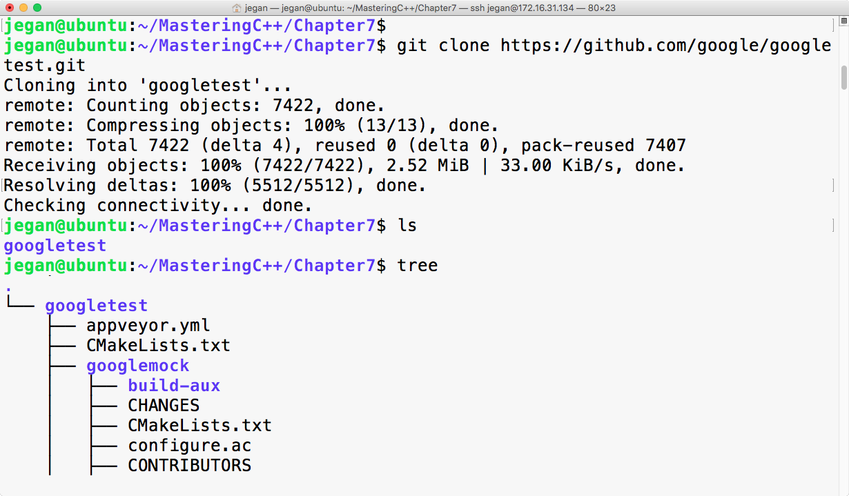
The googletest folder has both the googletest and googlemock frameworks in separate folders. Now we can invoke the cmake utility to configure our build and autogenerate Makefile, as follows:
cmake CMakeLists.txt
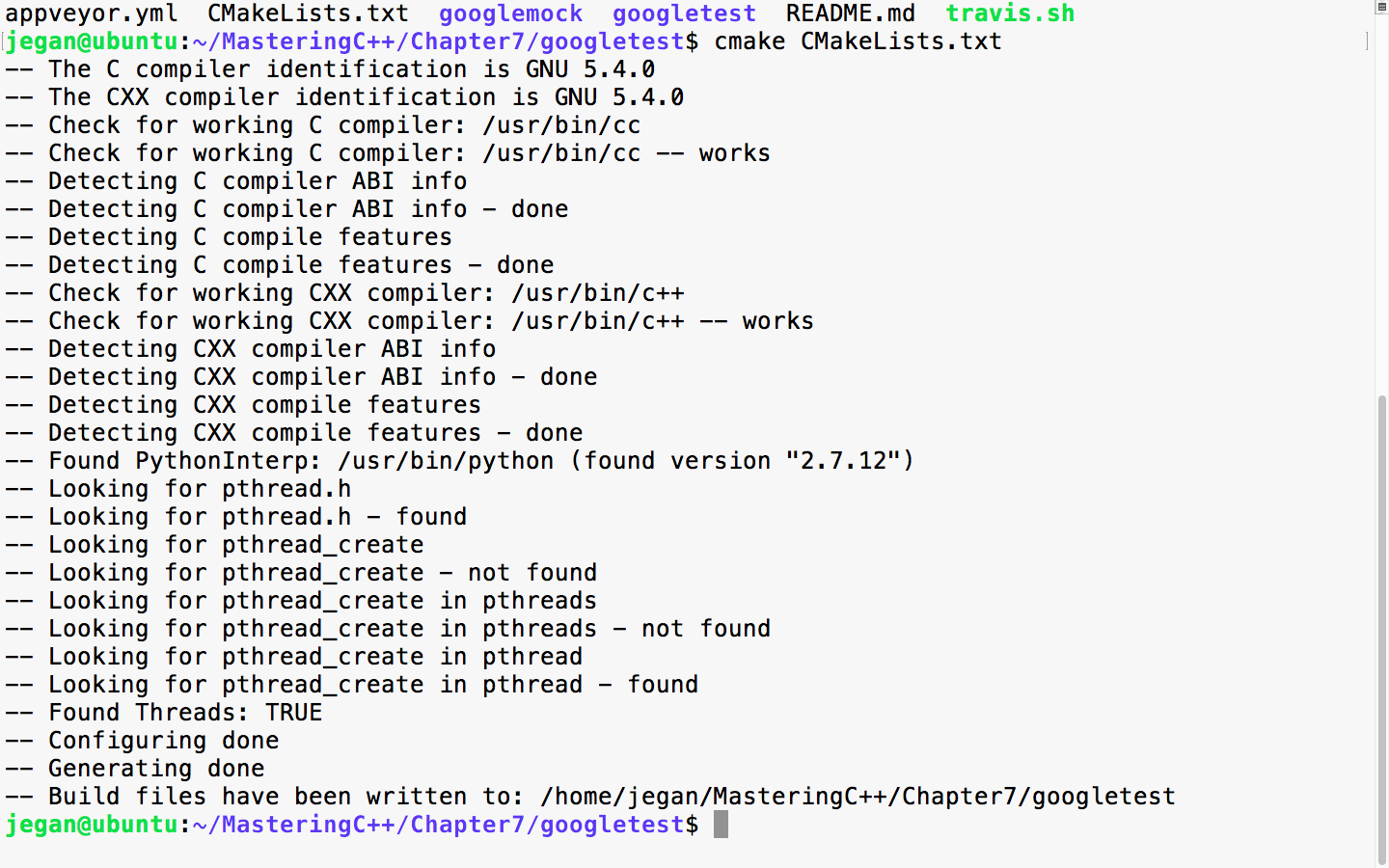
When the cmake utility is invoked, it detects the C/C++ header's files and its path that are necessary to build the Google test framework from the source code. Also, it will try to locate the tools required to build the source code. Once all the necessary headers and tools are located, it will autogenerate the Makefile. Once you have Makefile in place, you can use it to compile and install Google test and Google mock on your system:
sudo make install
The following screenshot demonstrates how you can install google test on your system:
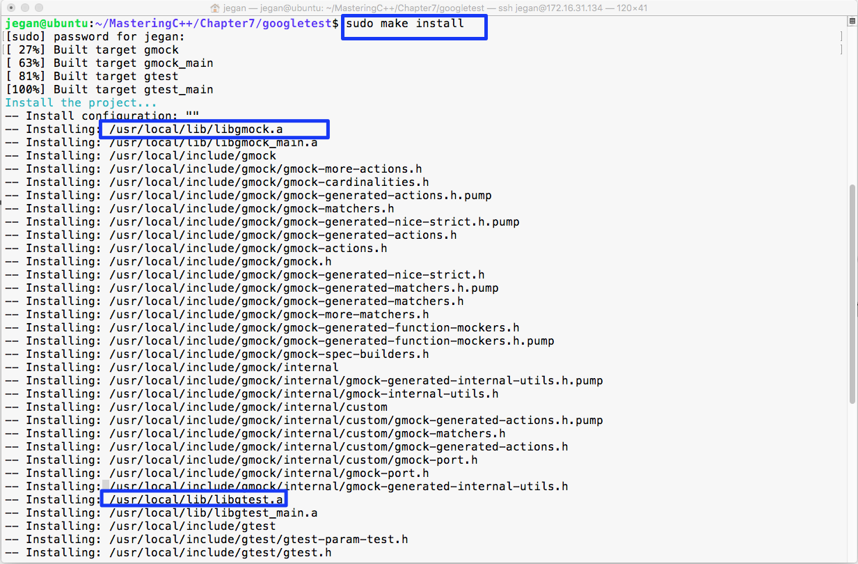
In the preceding image, the make install command has compiled and installed libgmock.a and libgtest.a static library files in the /usr/local/lib folder. Since the /usr/local/lib folder path is generally in the system's PATH environment variable, it can be accessed from any project within the system.
In case you don't prefer installing the libgmock.a and libgtest.a static library files and the respective header files on common system folders, then there is yet another way to build the Google test framework.
The following command will create three object files, as shown in Figure 7.4:
g++ -c googletest/googletest/src/gtest-all.cc googletest/googlemock/src/gmock-all.cc googletest/googlemock/src/gmock_main.cc -I googletest/googletest/ -I googletest/googletest/include -I googletest/googlemock -I googletest/googlemock/include -lpthread -
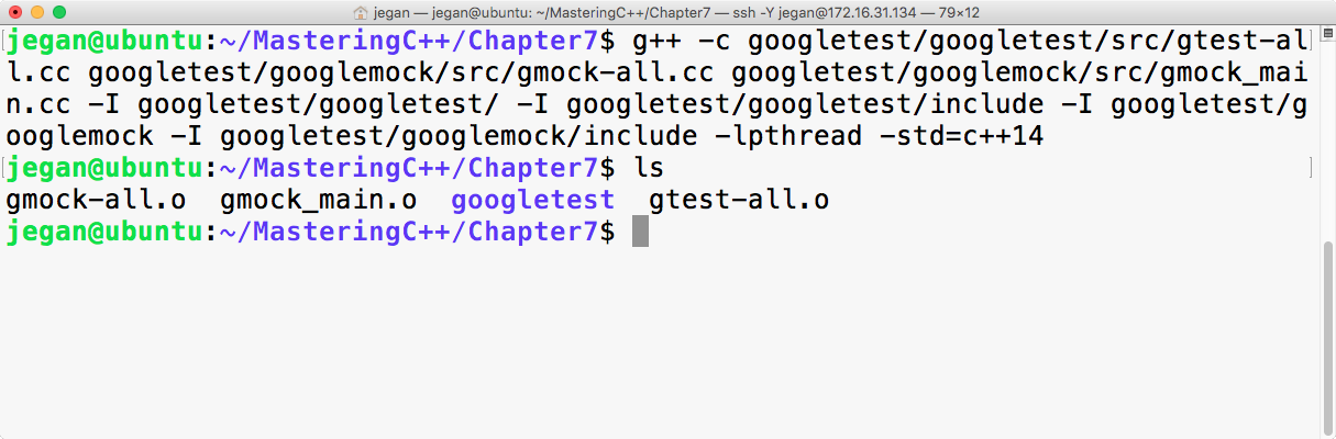
The next step is to combine all the object files into a single static library with the following command:
ar crf libgtest.a gmock-all.o gmock_main.o gtest-all.o
If all goes well, your folder should have the brand new libgtest.a static library, as shown in Figure 7.5. Let's understand the following command instructions:
g++ -c googletest/googletest/src/gtest-all.cc    googletest/googlemock/src/gmock-all.cc googletest/googlemock/src/gmock_main.cc -I googletest/googletest/ -I googletest/googletest/include
-I googletest/googlemock  -I googletest/googlemock/include -lpthread -std=c++14
The preceding command will help us create three object files: gtest-all.o, gmock-all.o, and gmock_main.o. The googletest framework makes use of some C++11 features, and I have purposefully used c++14 to be on the safer side. The gmock_main.cc source file has a main function that will initialize the Google mock framework, which in turn will internally initialize the Google test framework. The best part about this approach is that we don't have to supply the main function for our unit test application. Please note the compilation command includes the following include paths to help the g++ compiler locate the necessary header files in the Google test and Google mock frameworks:
-I googletest/googletest
-I googletest/googletest/include
-I googletest/googlemock
-I googletest/googlemock/include
Now the next step is to create our libgtest.a static library that will bundle both gtest and gmock frameworks into one single static library. As the Google test framework makes use of multiple threads, it is mandatory to link the pthread library as part of our static library:
ar crv libgtest.a gtest-all.o gmock_main.o gmock-all.o
The ar archive command helps combine all the object files into a single static library.
The following image demonstrates the discussed procedure practically in a terminal:
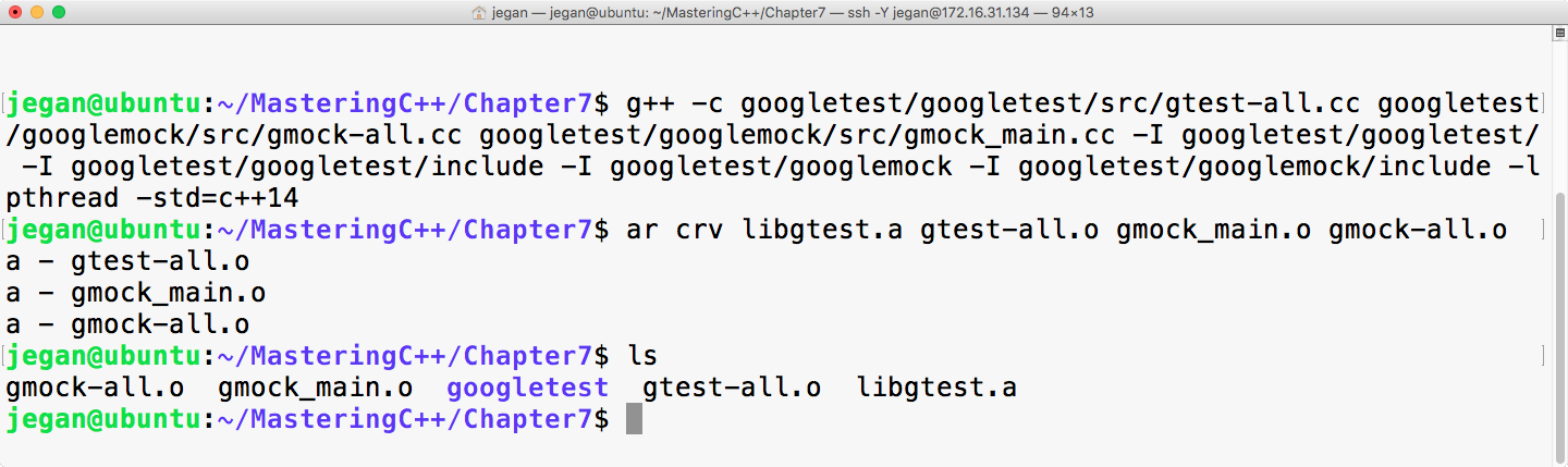
Learning the Google test framework is pretty easy. Let's create two folders: one for production code and the other for test code. The idea is to separate the production code from the test code. Once you have created both the folders, start with the Math.h header, as shown in Figure 7.6:
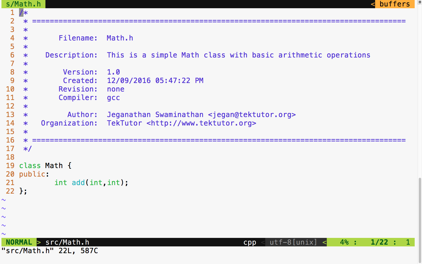
The Math class has just one function to demonstrate the usage of the unit test framework. To begin with, our Math class has a simple add function that is good enough to understand the basic usage of the Google test framework.
Let's implement our simple Math class in the following Math.cpp source file:
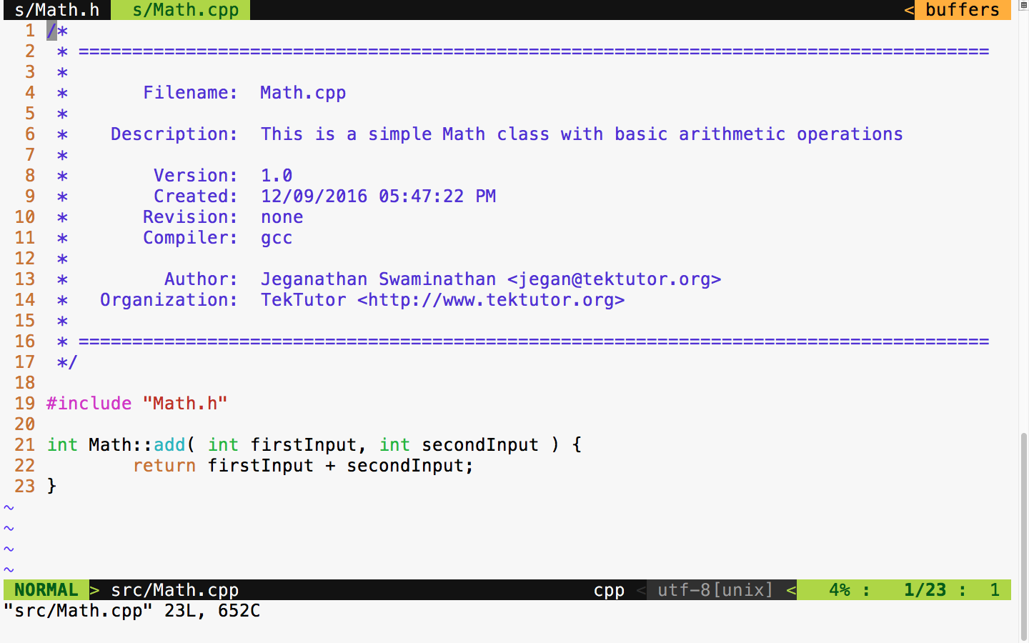
The preceding two files are supposed to be in the src folder, as shown in Figure 7.8. All of the production code gets into the src folder, and any number of files can be part of the src folder.
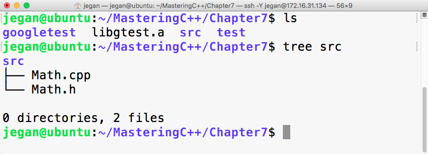
As we have written some production code, let's see how to write some basic test cases for the preceding production code. As a general best practice, it is recommended to name the test case file as either MobileTest or TestMobile so that it is easy for anyone to predict the purpose of the file. In C++ or in the Google test framework, it isn't mandatory to maintain the filename and class name as the same, but it is generally considered a best practice as it helps anyone locate a particular class just by looking at the filenames.
As we have already compiled our Google test framework as a static library, let's begin with the MathTest.cpp source file straight away:
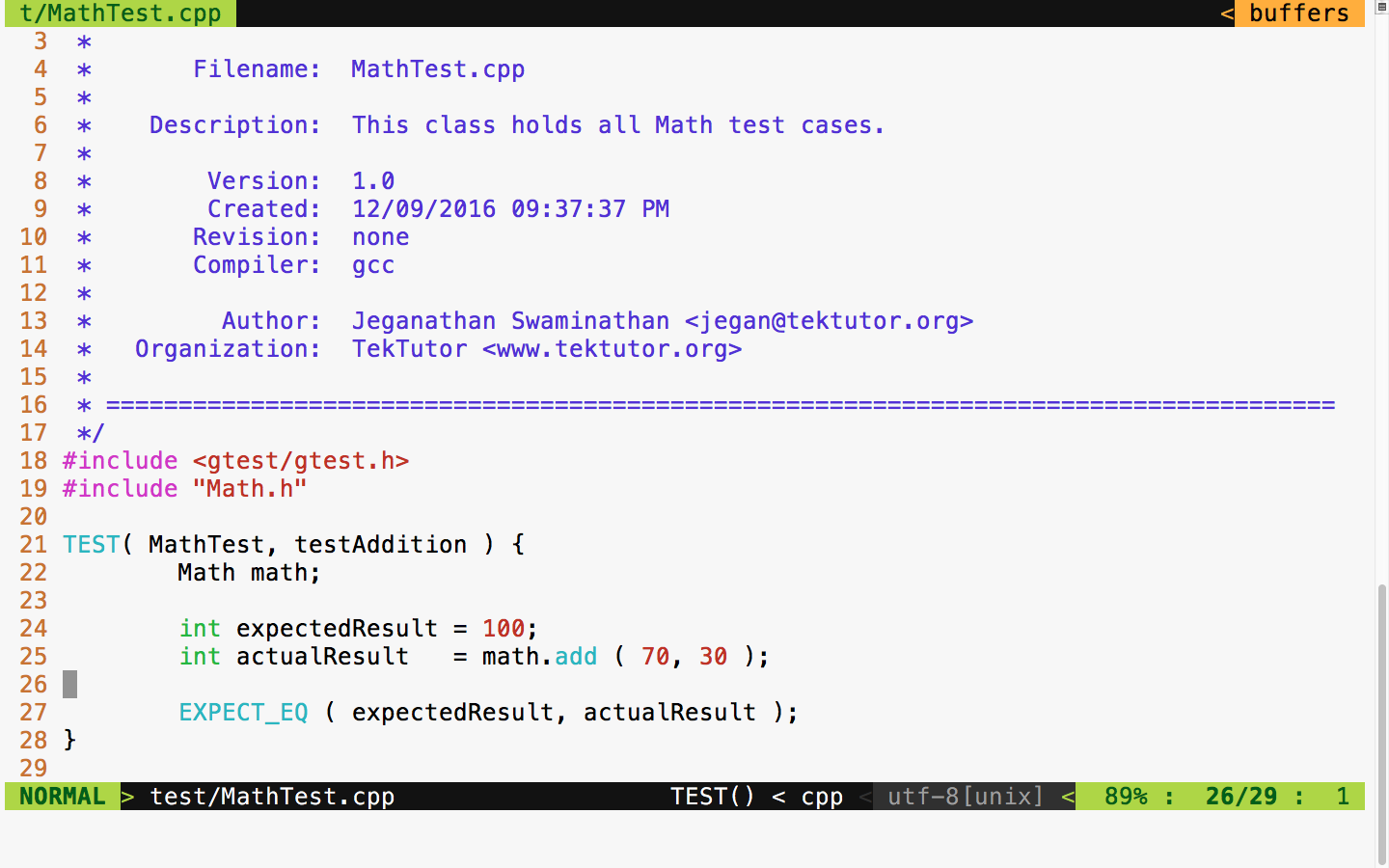
In Figure 7.9, at line number 18, we included the gtest header file from the Google test framework. In the Google test framework, test cases are written using a TEST macro that takes two parameters. The first parameter, namely MathTest, represents the test module name and the second parameter is the name of the test case. Test modules help us group a bunch of related test cases under a module. Hence, it is very important to name the test module and test case aptly to improve the readability of the test report.
As you are aware, Math is the class we are intending to test; we have instantiated an object of the Math object at line 22. In line 25, we invoked the add function on the math object, which is supposed to return the actual result. Finally, at line 27, we checked whether the expected result matches the actual result. The Google test macro EXPECT_EQ will mark the test case as passed if the expected and actual result match; otherwise, the framework will mark the test case outcome as failed.
Cool, we are all set now. Let's see how to compile and run our test case now. The following command should help you compile the test case:
g++ -o tester.exe src/Math.cpp test/MathTest.cpp -I googletest/googletest
-I googletest/googletest/include -I googletest/googlemock
-I googletest/googlemock/include -I src libgtest.a -lpthread
Note that the compilation command includes the following include path:
-I googletest/googletest
-I googletest/googletest/include
-I googletest/googlemock
-I googletest/googlemock/include
-I src
Also, it is important to note that we also linked our Google test static library libgtest.a and the POSIX pthreads library as the Google test framework makes use of multiple .
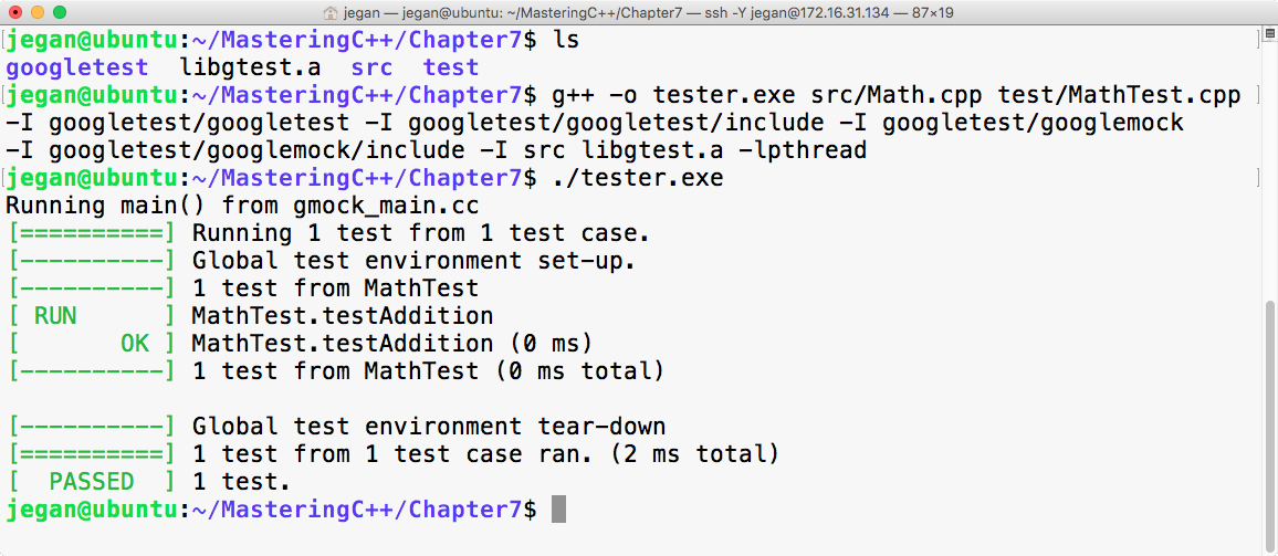
Congrats! We have compiled and executed our first test case successfully.
First, we need to download the Google test framework .zip file from https://github.com/google/googletest/archive/master.zip. The next step is to extract the .zip file in some directory. In my case, I have extracted it into the googletest folder and copied all the contents of googletest googletest-mastergoogletest-master to the googletest folder, as shown in Figure 7.11:
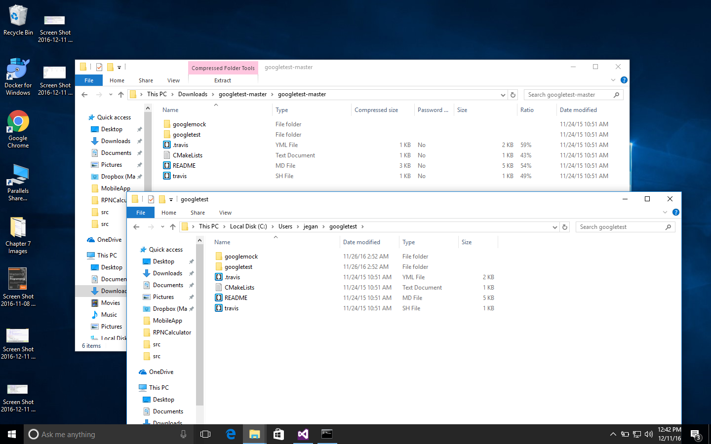
It is time to create a simple project in Visual Studio. I have used Microsoft Visual Studio Community 2015. However, the procedure followed here should pretty much remain the same for other versions of Visual Studio, except that the options might be available in different menus.
You need to create a new project named MathApp by navigating to New Project | Visual Studio | Windows | Win32 | Win32 Console Application, as shown in Figure 7.12. This project is going to be the production code to be tested.

Let's add the MyMath class to the MathApp project. The MyMath class is the production code that will be declared in MyMath.h and defined in MyMath.cpp.
Let's take a look at the MyMath.h header file shown in Figure 7.13:
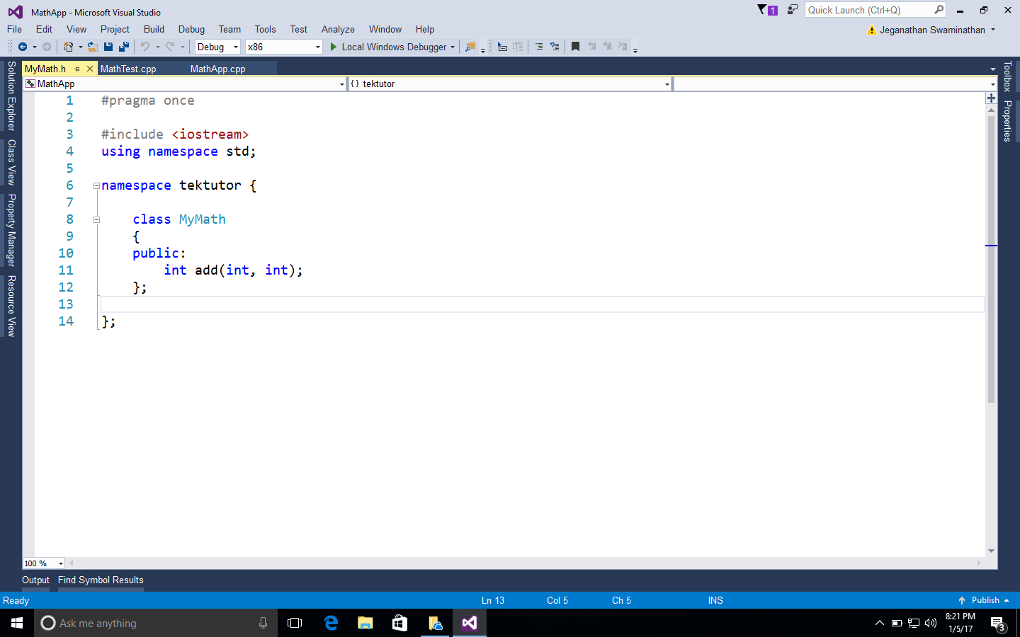
The definition of the MyMath class looks as shown in Figure 7.14:
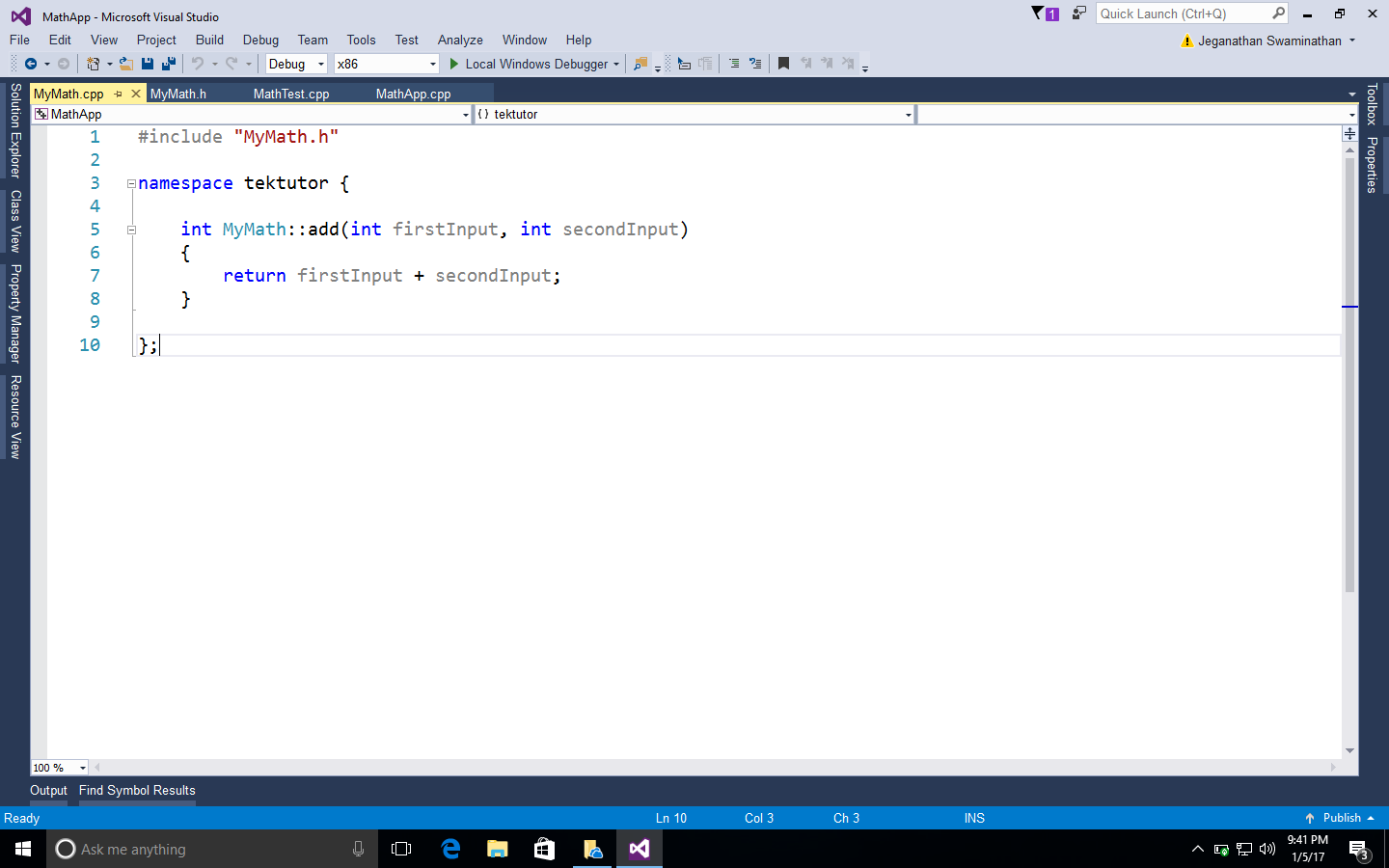
As it is a console application, it is mandatory to supply the main function, as shown in Figure 7.15:
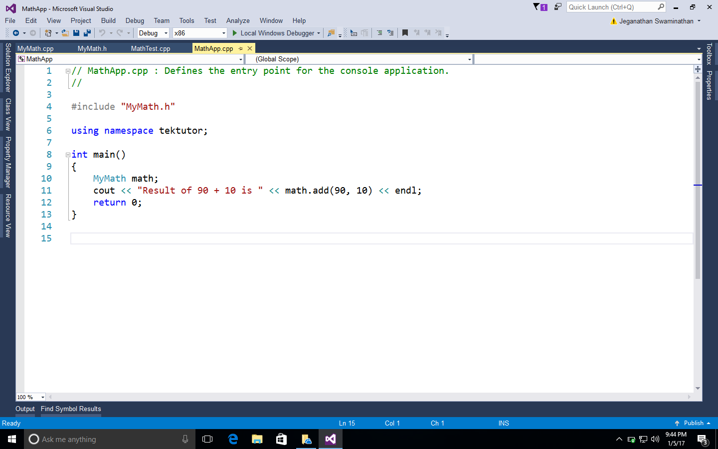
Next, we are going to add a static library project named GoogleTestLib to the same MathApp project solution, as shown in Figure 7.16:
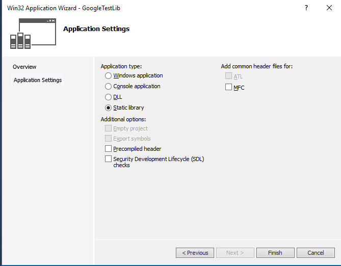
Next, we need to add the following source files from the Google test framework to our static library project:
C:Usersjegangoogletestgoogletestsrcgtest-all.cc
C:Usersjegangoogletestgooglemocksrcgmock-all.cc
C:Usersjegangoogletestgooglemocksrcgmock_main.cc
In order to compile the static library, we need to include the following header file paths in GoogleTestLib/Properties/VC++ Directories/Include directories:
C:Usersjegangoogletestgoogletest
C:Usersjegangoogletestgoogletestinclude
C:Usersjegangoogletestgooglemock
C:Usersjegangoogletestgooglemockinclude
You may have to customize the paths based on where you have copied/installed the Google test framework in your system.
Now it's time to add the MathTestApp Win32 console application to the MathApp solution. We need to make MathTestApp as a StartUp project so that we can directly execute this application. Let's ensure there are no source files in the MathTestApp project before we add a new source file named MathTest.cpp to the MathTestApp project.
We need to configure the same set of Google test framework include paths we added to the GoogleTestLib static library. In addition to this, we must also add the MathApp project directory as the test project will refer to the header file in the MathApp project, as follows. However, customize the paths as per the directory structure you follow for this project in your system:
C:Usersjegangoogletestgoogletest
C:Usersjegangoogletestgoogletestinclude
C:Usersjegangoogletestgooglemock
C:Usersjegangoogletestgooglemockinclude
C:ProjectsMasteringC++ProgrammingMathAppMathApp
In the MathAppTest project, make sure you have added references to MathApp and GoogleTestLib so that the MathAppTest project will compile the other two projects when it senses changes in them.
Great! We are almost done. Now let's implement MathTest.cpp, as shown in Figure 7.17:
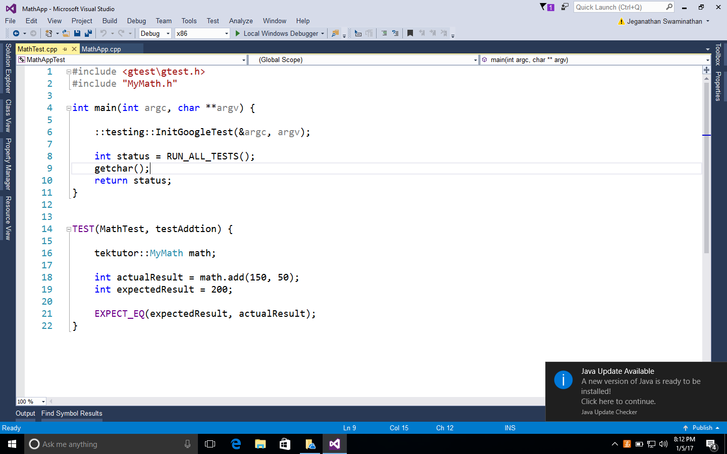
Everything is ready now; let's run the test cases and check the result:
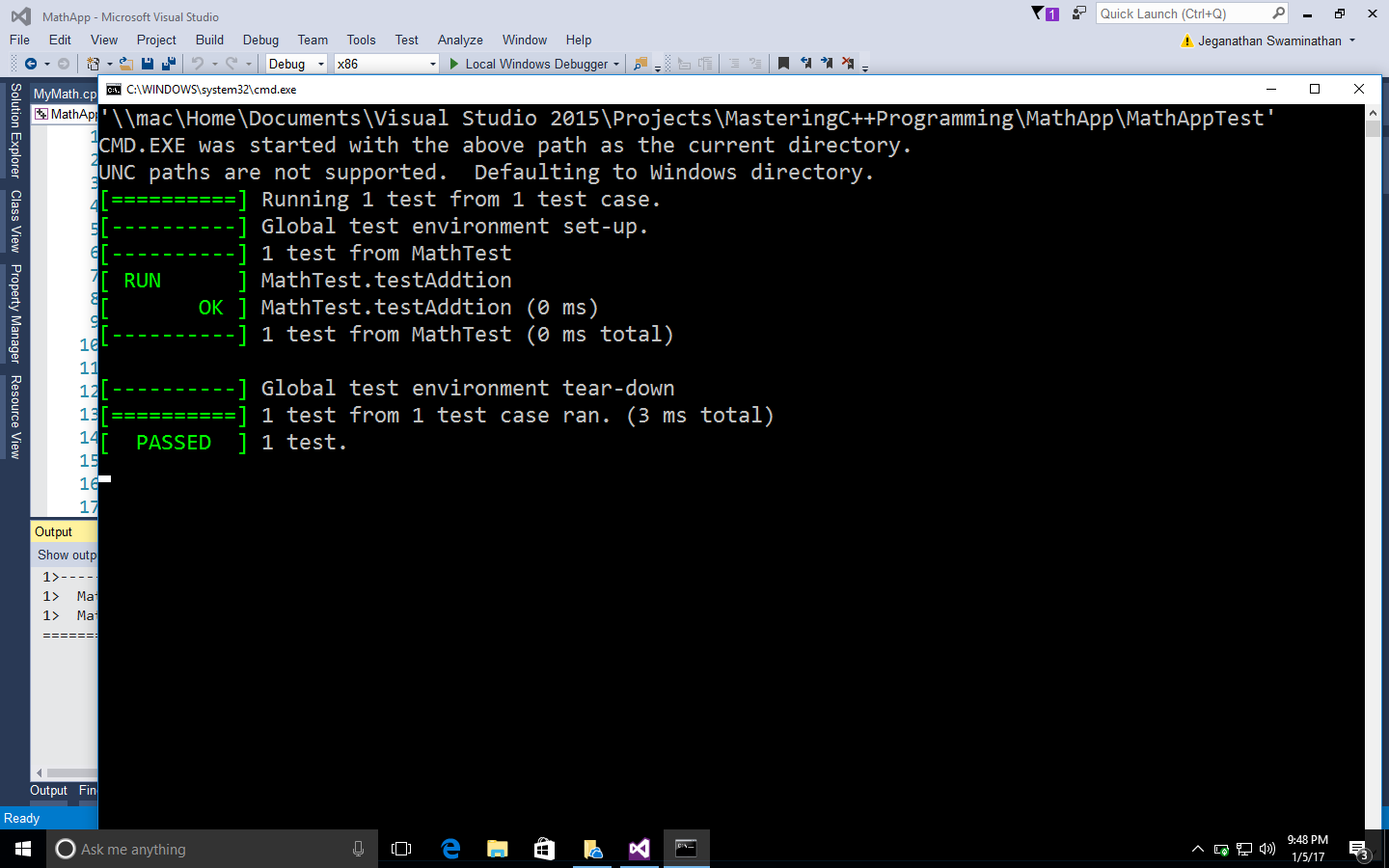
Let's see how to develop an Reverse Polish Notation (RPN) calculator application that follows the TDD approach. RPN is also known as the postfix notation. The expectation from the RPN Calculator application is to accept a postfix math expression as an input and return the evaluated result as the output.
Step by step, I would like to demonstrate how one can follow the TDD approach while developing an application. As the first step, I would like to explain the project directory structure, then we'll move forward. Let's create a folder named Ex2 with the following structure:
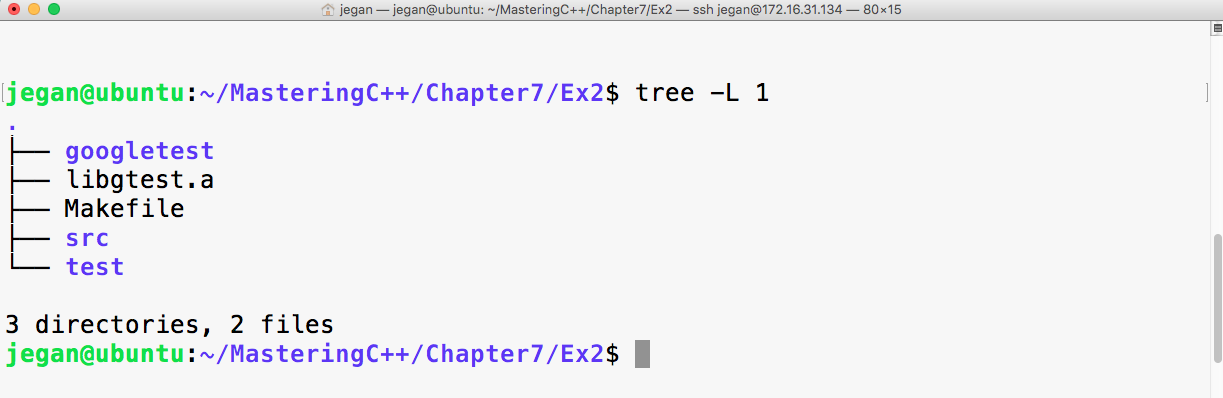
The googletest folder is the gtest test library that has the necessary gtest and gmock header files. Now libgtest.a is the Google test static library that we created in the previous exercise. We are going to use the make utility to build our project, hence I have placed a Makefile in the project home directory. The src directory will hold the production code, while the test directory will hold all the test cases that we are going to write.
Before we start writing test cases, let's take a postfix math "2 5 * 4 + 3 3 * 1 + /" and understand the standard postfix algorithm that we are going to apply to evaluate the RPN math expression. As per the postfix algorithm, we are going to parse the RPN math expression one token at a time. Whenever we encounter an operand (number), we are going to push that into the stack. Whenever we encounter an operator, we are going to pop out two values from the stack, apply the math operation, push back the intermediate result into the stack, and repeat the procedure until all the tokens are evaluated in the RPN expression. At the end, when no more tokens are left in the input string, we will pop out the value and print it as the result. The procedure is demonstrated step by step in the following figure:
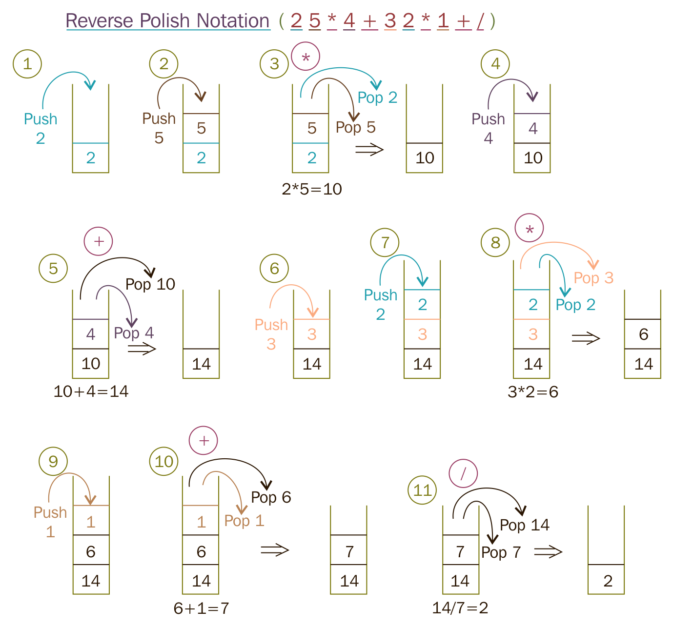
To start with, let's take a simple postfix math expression and translate the scenario into a test case:
Test Case : Test a simple addition
Input: "10 15 +"
Expected Output: 25.0
Let's translate the preceding test case as a Google test in the test folder, as follows:
test/RPNCalculatorTest.cpp

TEST ( RPNCalculatorTest, testSimpleAddition ) {
         RPNCalculator rpnCalculator;
         double actualResult = rpnCalculator.evaluate ( "10 15 +" );
         double expectedResult = 25.0;
         EXPECT_EQ ( expectedResult, actualResult );
}
In order to compile the preceding test case, let's write the minimal production code that is required in the src folder, as follows:
src/RPNCalculator.h

#include <iostream>
#include <string>
using namespace std;

class RPNCalculator {
  public:
      double evaluate ( string );
};
As the RPN math expression will be supplied as a space-separated string, the evaluate method will take a string input argument:
src/RPNCalculator.cpp

#include "RPNCalculator.h"

double RPNCalculator::evaluate ( string rpnMathExpression ) {
    return 0.0;
}
The following Makefile class helps run the test cases every time we compile the production code:
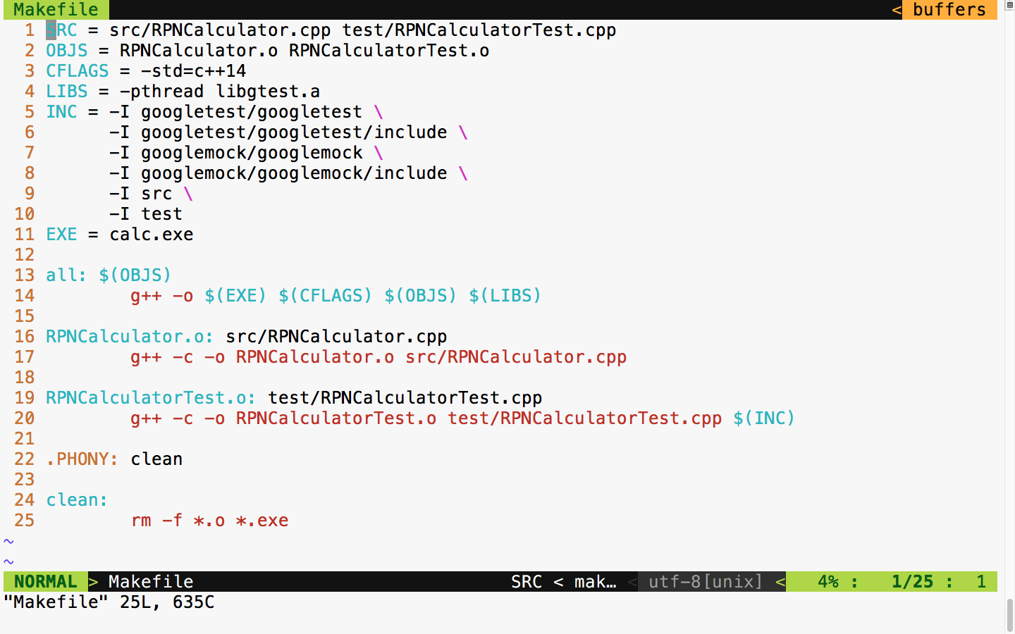
Now let's build and run the test case and check the test case's outcome:
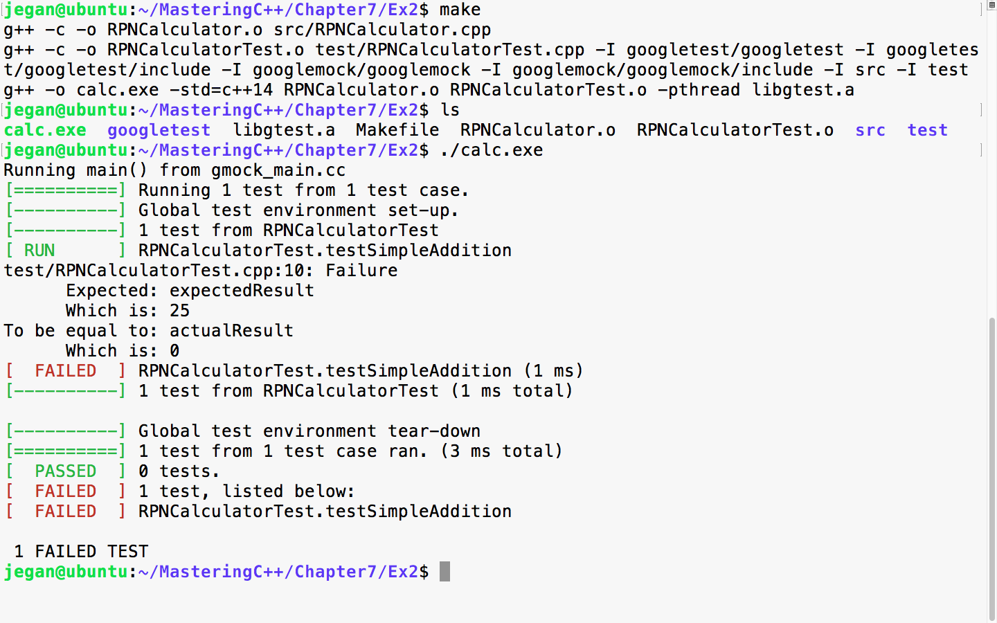
In TDD, we always start with a failing test case. The root cause of the failure is that the expected result is 25, while the actual result is 0. The reason is that we haven't implemented the evaluate method, hence we have hardcoded to return 0, irrespective of any input. So let's implement the evaluate method in order to make the test case pass.
We need to modify src/RPNCalculator.h and src/RPNCalculator.cpp as follows:
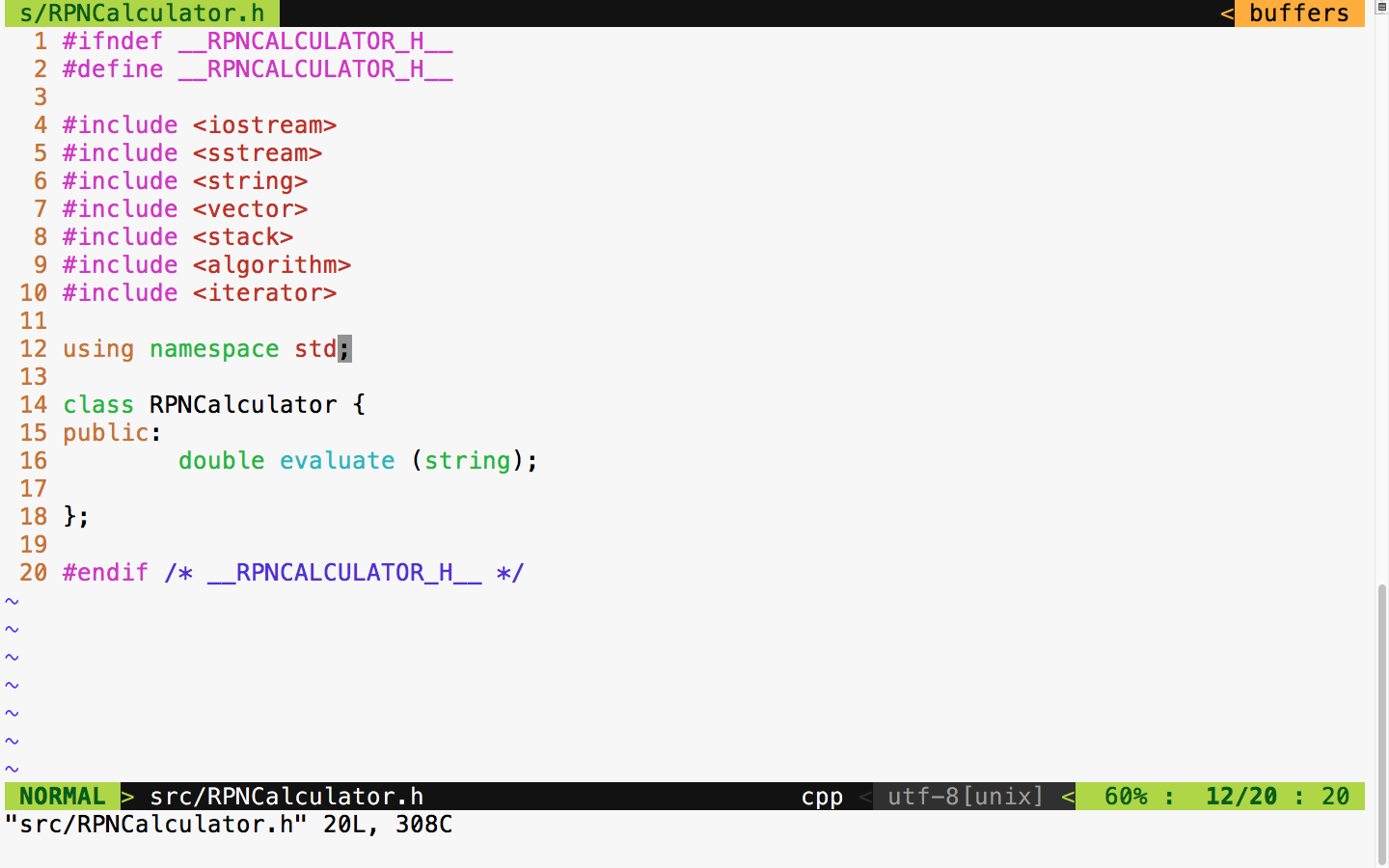
In the RPNCalculator.h header file, observe the new header files that are included to handle string tokenizing and string double conversion and copy the RPN tokens to the vector:
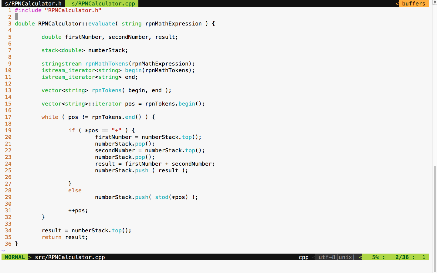
As per the standard postfix algorithm, we are using a stack to hold all the numbers that we find in the RPN expression. Anytime we encounter the + math operator, we pop out two values from the stack and add them and push back the results into the stack. If the token isn't a + operator, we can safely assume that it would be a number, so we just push the value to the stack.
With the preceding implementation in place, let's try the test case and check whether the test case passes:
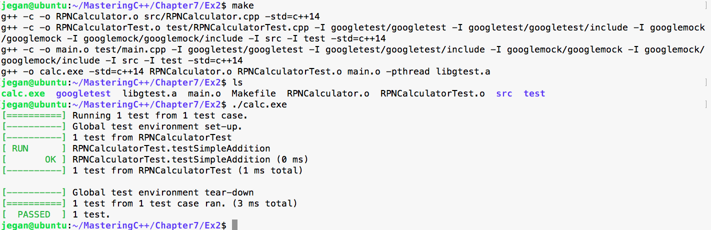
Cool, our first test case has passed as expected. It's time to think of another test case. This time, let's add a test case for subtraction:
Test Case : Test a simple subtraction
Input: "25 10 -"
Expected Output: 15.0
Let's translate the preceding test case as a Google test in the test folder, as follows:
test/RPNCalculatorTest.cpp

TEST ( RPNCalculatorTest, testSimpleSubtraction ) {
         RPNCalculator rpnCalculator;
         double actualResult = rpnCalculator.evaluate ( "25 10 -" );
         double expectedResult = 15.0;
         EXPECT_EQ ( expectedResult, actualResult );
}
With the preceding test case added to test/RPNCalculatorTest, it should now look like this:
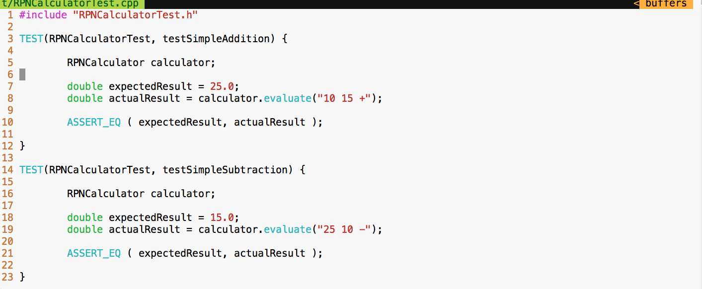
Let's execute the test cases and check whether our new test case passes:
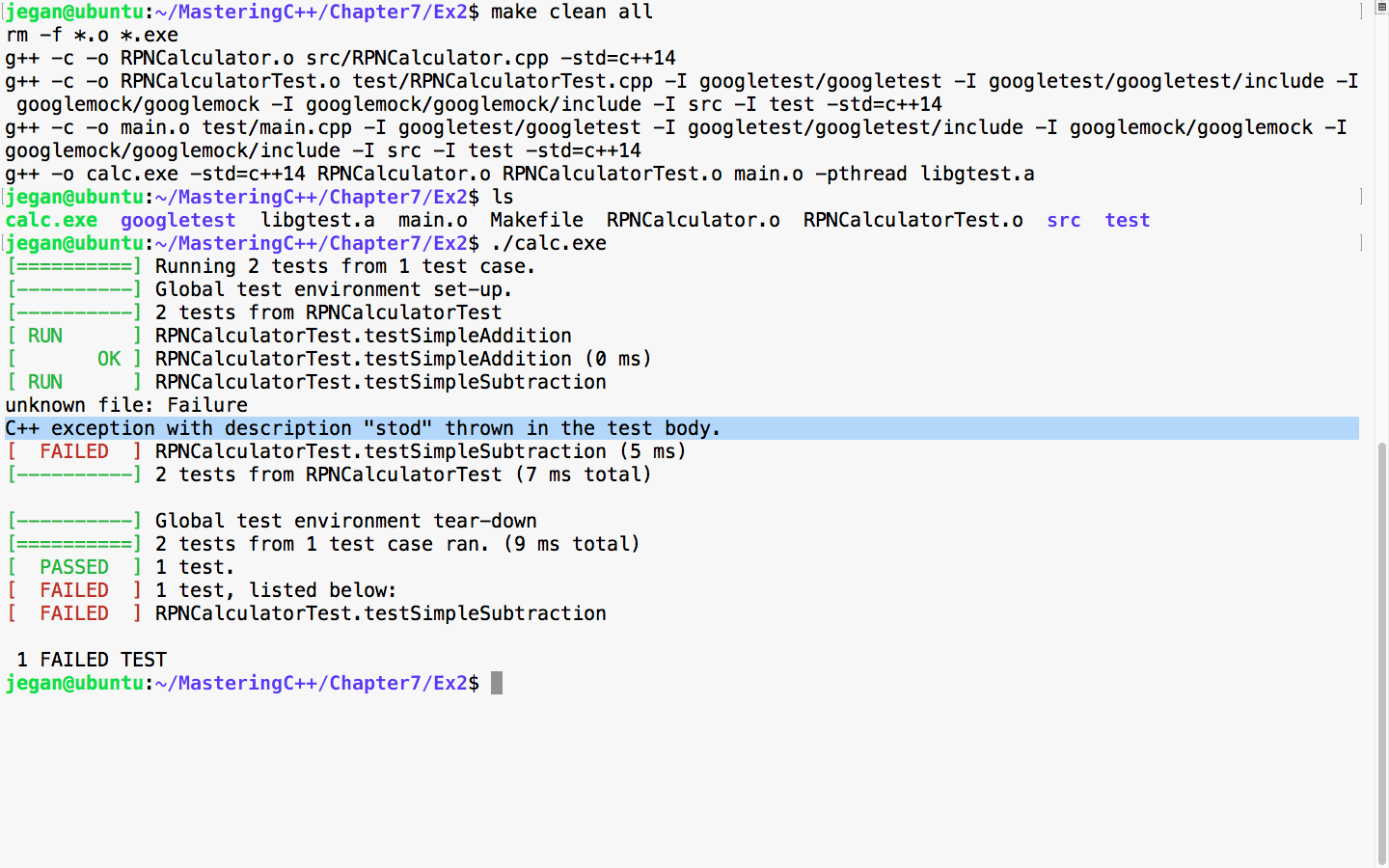
As expected, the new test fails as we haven't added support for subtraction in our application yet. This is very evident, based on the C++ exception, as the code attempts to convert the subtraction - operator into a number. Let's add support for subtraction logic in our evaluate method:
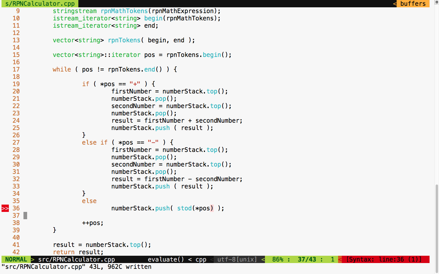
It's time to test. Let's execute the test case and check whether things are working:
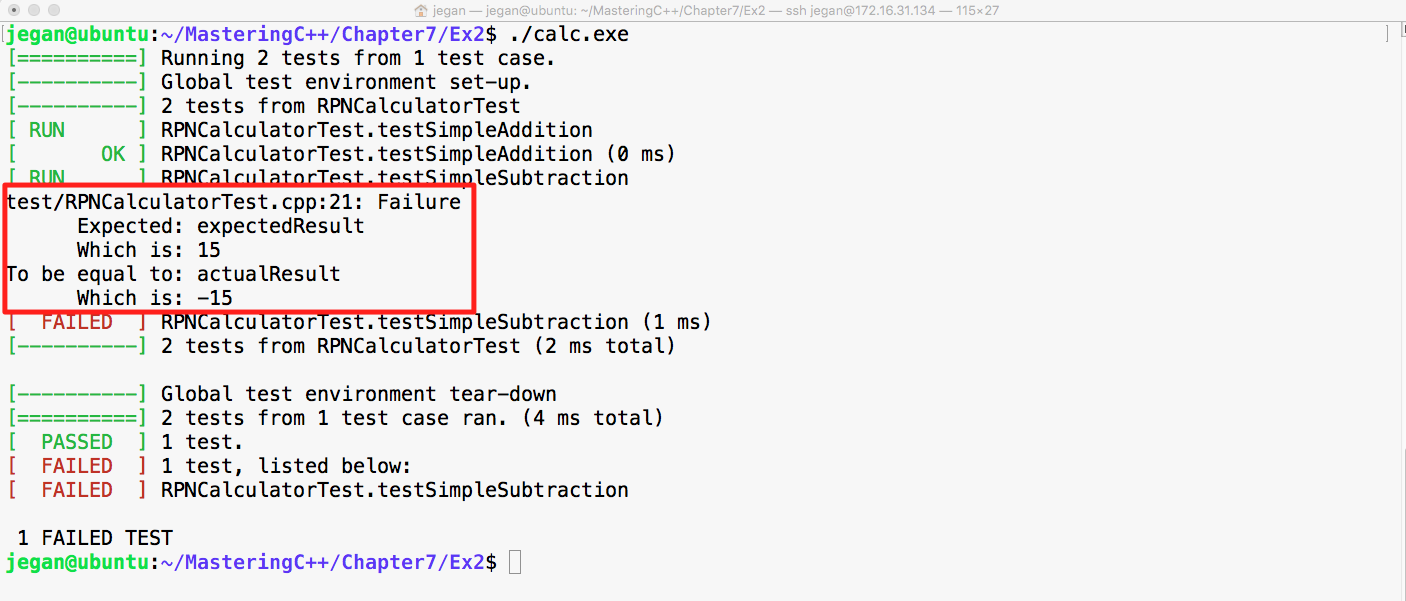
Cool! Did you notice that our test case failed in this instance? Wait a minute. Why are we excited if the test case failed? The reason we should be happy is that our test case found a bug; after all, that is the main intent of TDD, isn't?
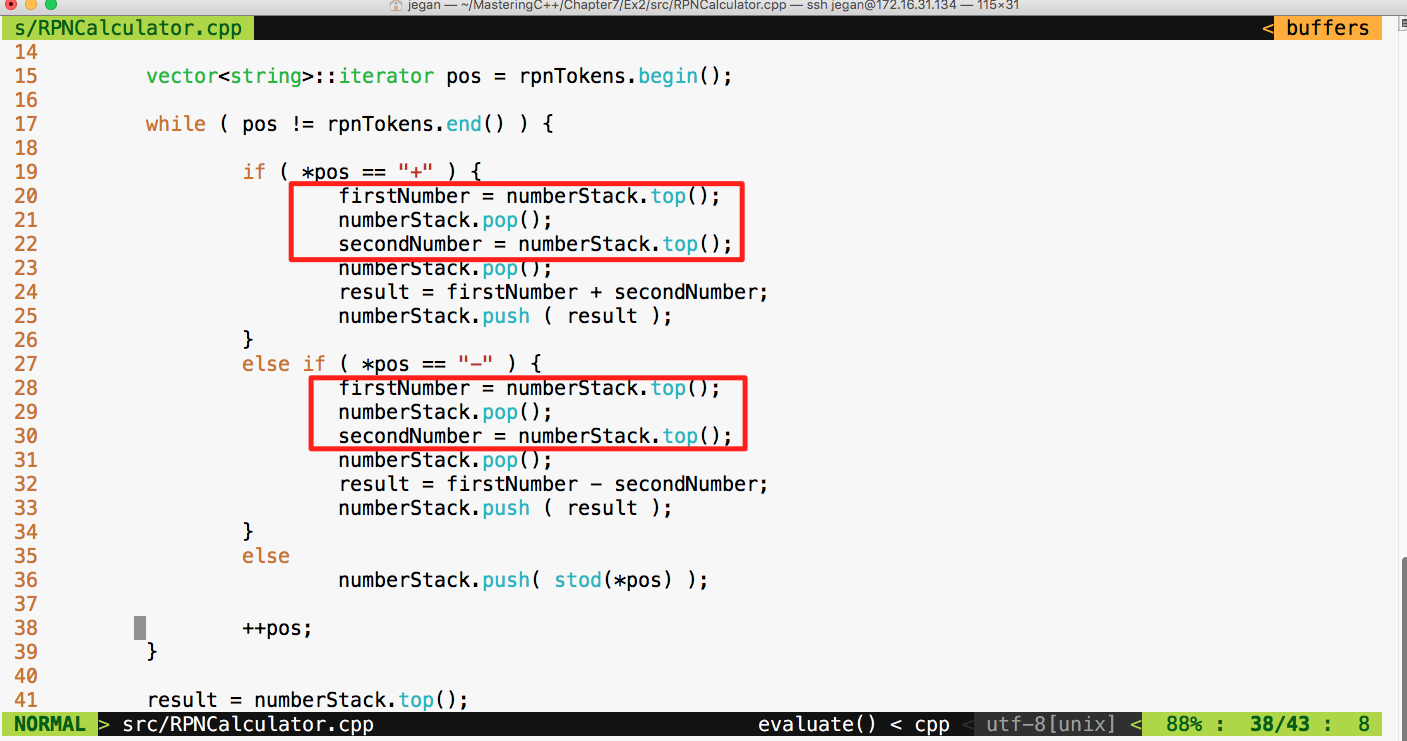
The root cause of the failure is that the Stack operates on the basis of Last In First Out (LIFO) whereas our code assumes FIFO. Did you notice that our code assumes that it will pop out the first number first while the reality is that it is supposed to pop out the second number first? Interesting, this bug was there in the addition operation too; however, since addition is associative, the bug was kind of suppressed but the subtraction test case detected it.
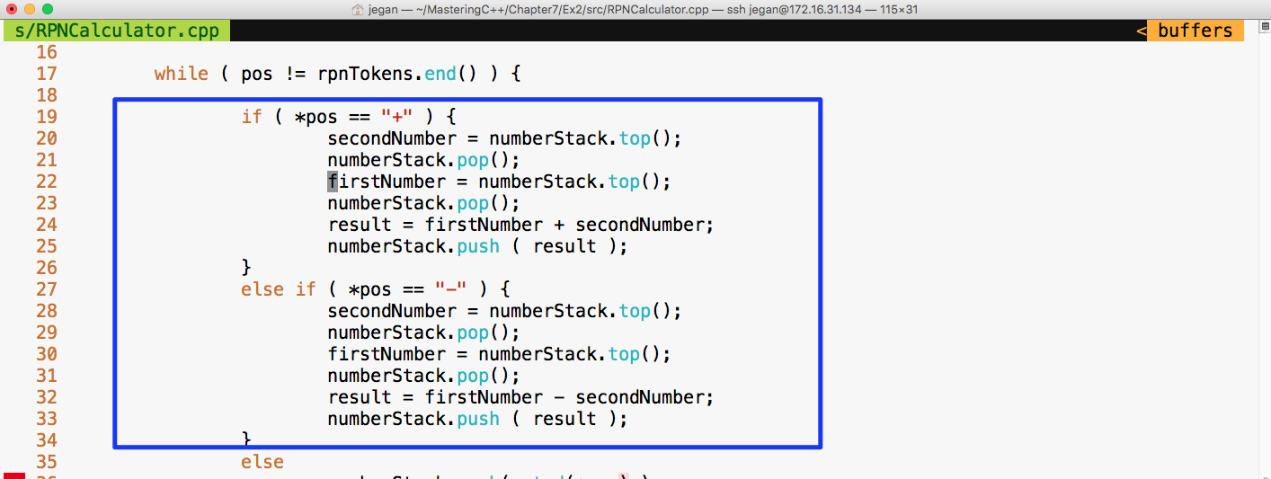
Let's fix the bug as shown in the preceding screenshot and check whether the test cases will pass:
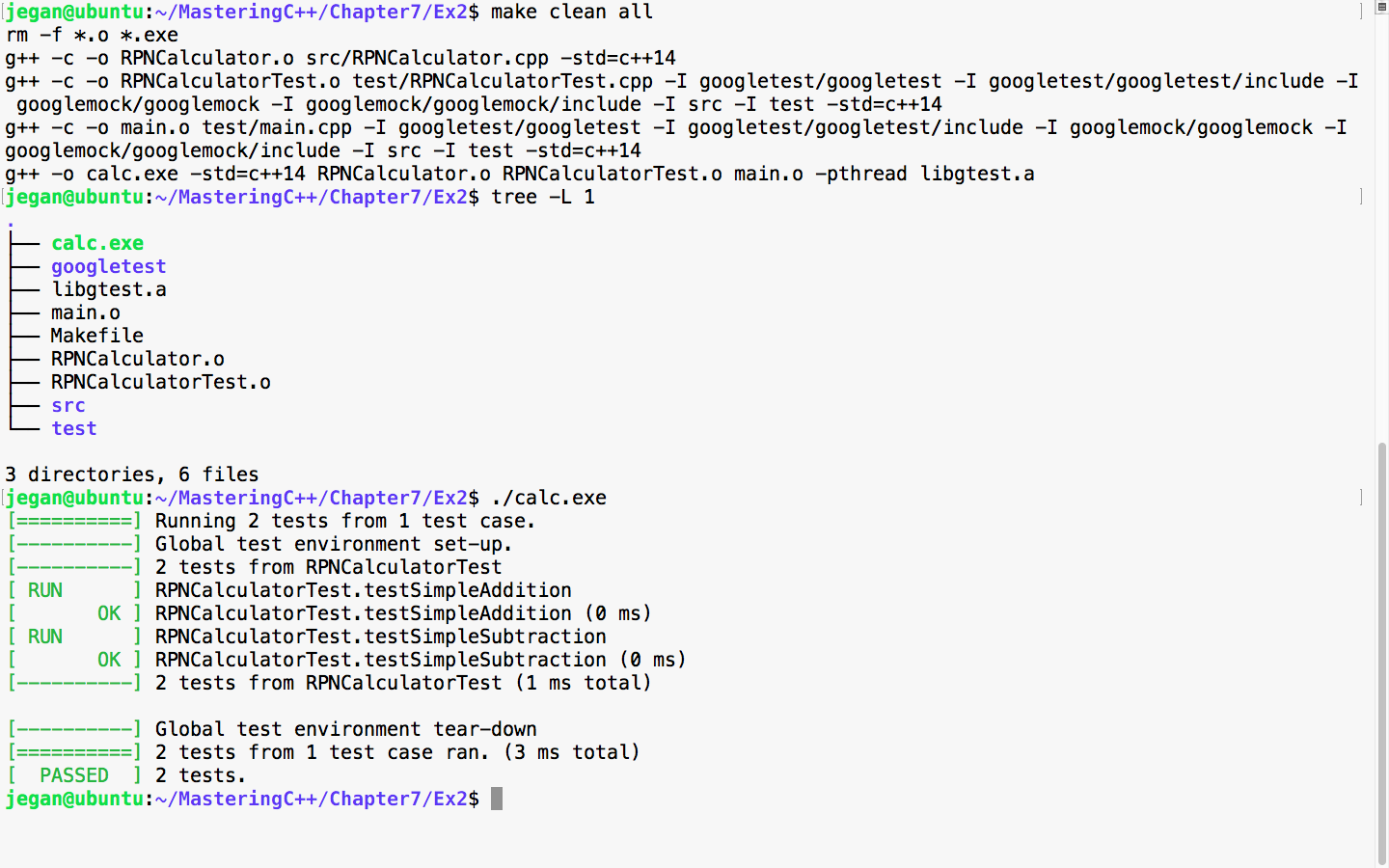
Awesome! We fixed the bug and our test case seems to certify they are fixed. Let's add more test cases. This time, let's add a test case to verify multiplication:
Test Case : Test a simple multiplication
Input: "25 10 *"
Expected Output: 250.0
Let's translate the preceding test case as a google test in the test folder, as follows:
test/RPNCalculatorTest.cpp

TEST ( RPNCalculatorTest, testSimpleMultiplication ) {
         RPNCalculator rpnCalculator;
         double actualResult = rpnCalculator.evaluate ( "25 10 *" );
         double expectedResult = 250.0;
         EXPECT_EQ ( expectedResult, actualResult );
}
We know this time the test case is going to fail, so let's fast forward and take a look at the division test case:
Test Case : Test a simple division
Input: "250 10 /"
Expected Output: 25.0
Let's translate the preceding test case as a google test in the test folder, as follows:
test/RPNCalculatorTest.cpp

TEST ( RPNCalculatorTest, testSimpleDivision ) {
         RPNCalculator rpnCalculator;
         double actualResult = rpnCalculator.evaluate ( "250 10 /" );
         double expectedResult = 25.0;
         EXPECT_EQ ( expectedResult, actualResult );
}
Let's skip the test result and move forward with a final complex expression test case that involves many operations:
Test Case : Test a complex rpn expression
Input: "2  5  *  4  + 7  2 -  1  +  /"
Expected Output: 25.0
Let's translate the preceding test case as a google test in the test folder, as shown here:
test/RPNCalculatorTest.cpp

TEST ( RPNCalculatorTest, testSimpleDivision ) {
         RPNCalculator rpnCalculator;
         double actualResult = rpnCalculator.evaluate ( "250 10 /" );
         double expectedResult = 25.0;
         EXPECT_EQ ( expectedResult, actualResult );
}
Let's check whether our RPNCalculator application is able to evaluate a complex RPN expression that involves addition, subtraction, multiplication, and division in a single expression with the following test case:
test/RPNCalculatorTest.cpp

TEST ( RPNCalculatorTest, testComplexExpression ) {
         RPNCalculator rpnCalculator;
         double actualResult = rpnCalculator.evaluate ( "2  5  *  4  +  7  2 - 1 +  /" );
         double expectedResult = 2.33333;
         ASSERT_NEAR ( expectedResult, actualResult, 4 );
}
In the preceding test case, we are checking whether the expected result matches the actual result to the approximation of up to four decimal places. If the values are different beyond this approximation, then the test case is supposed to fail.
Let's check the test case output now:
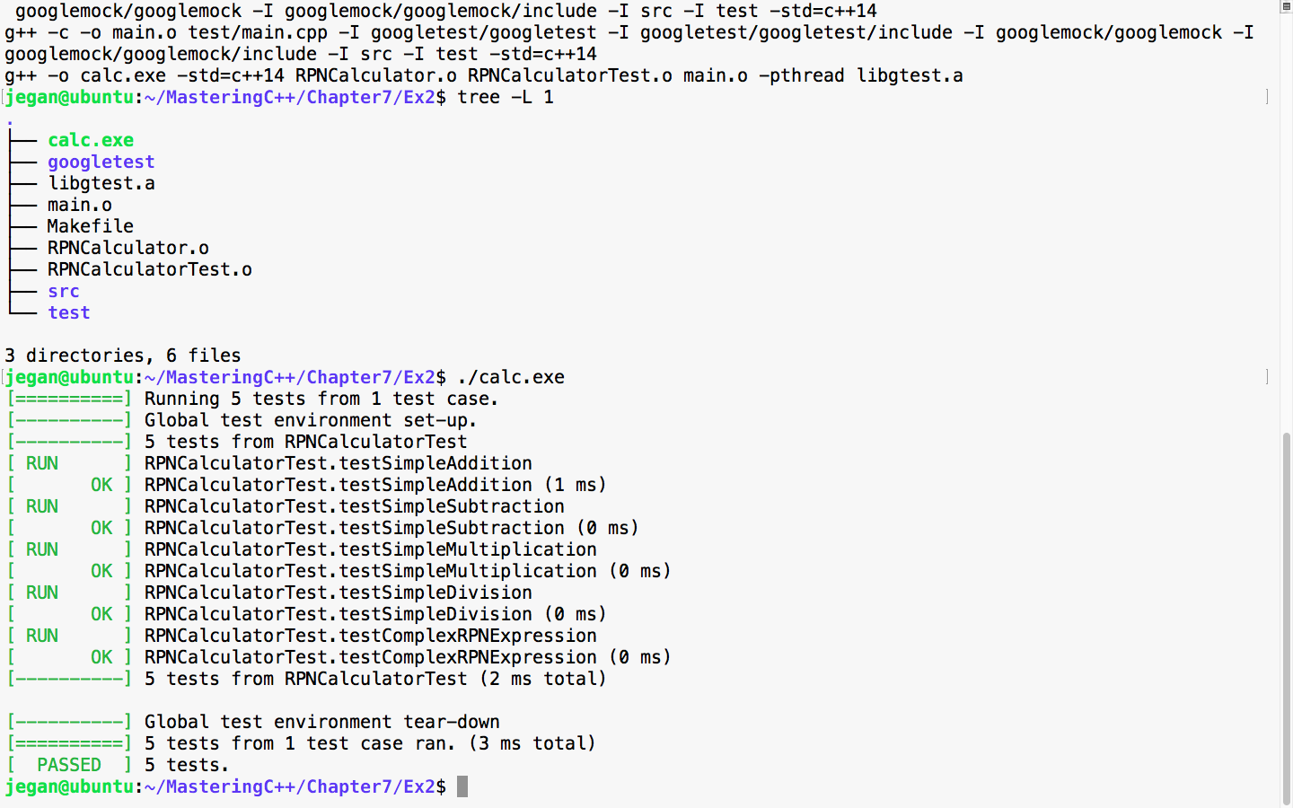
Great! All the test cases are green.
Now let's take a look at our production code and check whether there is any room for improvement:
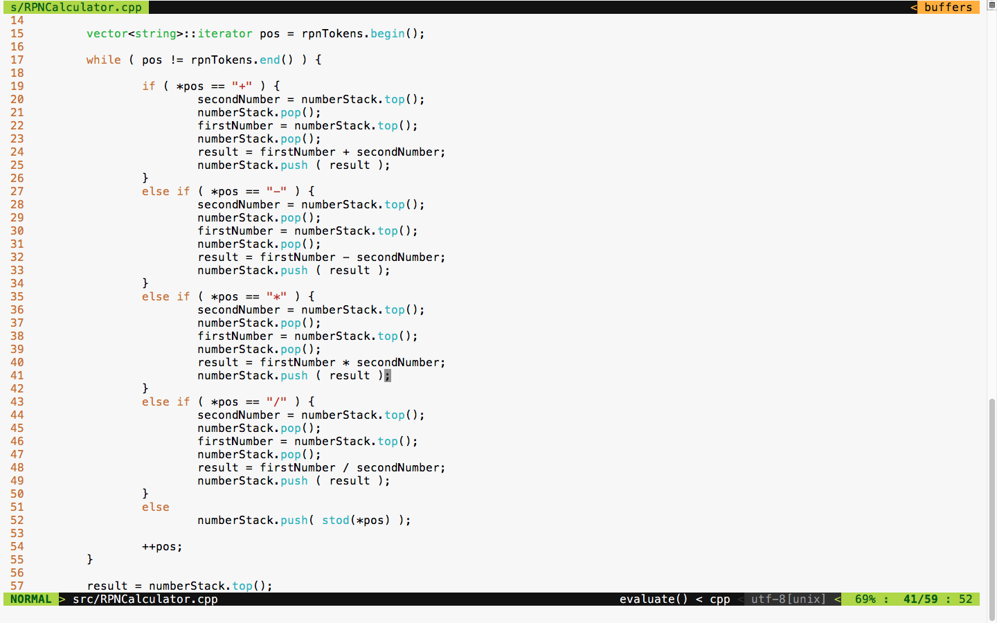
The code is functionally good but has many code smells. It is a long method with the nested if-else condition and duplicate code. TDD is not just about test automation; it is also about writing good code without code smells. Hence, we must refactor code and make it more modular and reduce the code complexity.
We can apply polymorphism or the strategy design pattern here instead of the nested if-else conditions. Also, we can use the factory method design pattern to create various subtypes. There is also scope to use the Null Object Design Pattern.
The best part is we don't have to worry about the risk of breaking our code in the process of refactoring as we have a sufficient number of test cases to give us feedback in case we break our code.
First, let's understand how we could refactor the RPNCalculator design shown in Figure 7.35:
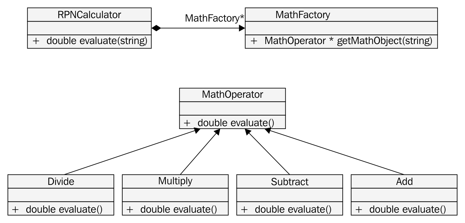
Based on the preceding design refactoring approach, we can refactor RPNCalculator as shown in Figure 7.36:
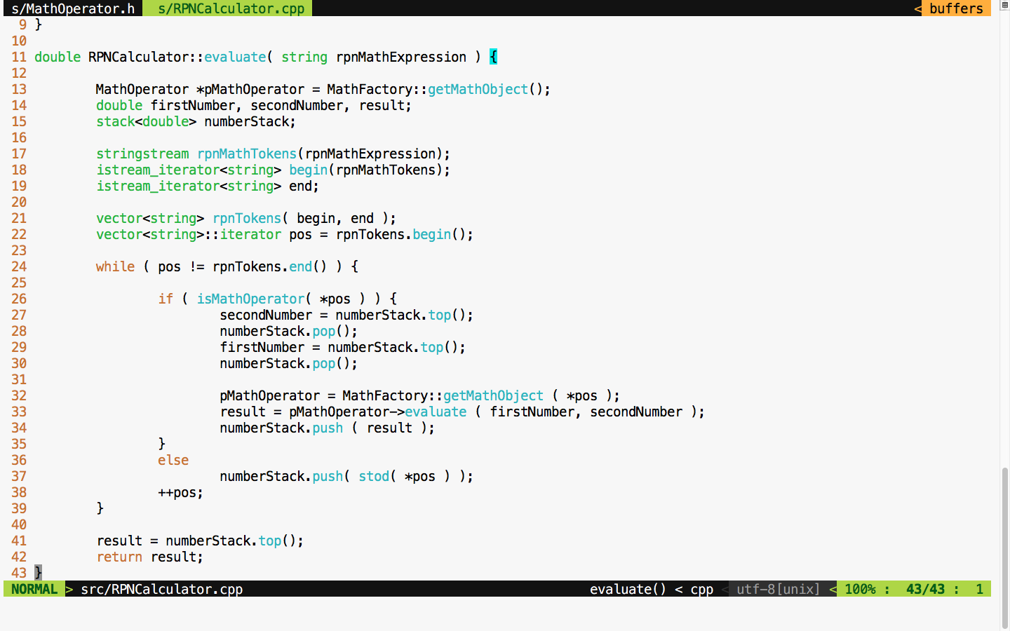
If you compare the RPNCalculator code before and after refactoring, you'll find that code complexity has reduced to a decent amount after refactoring.
The MathFactory class can be implemented as shown in Figure 7.37:
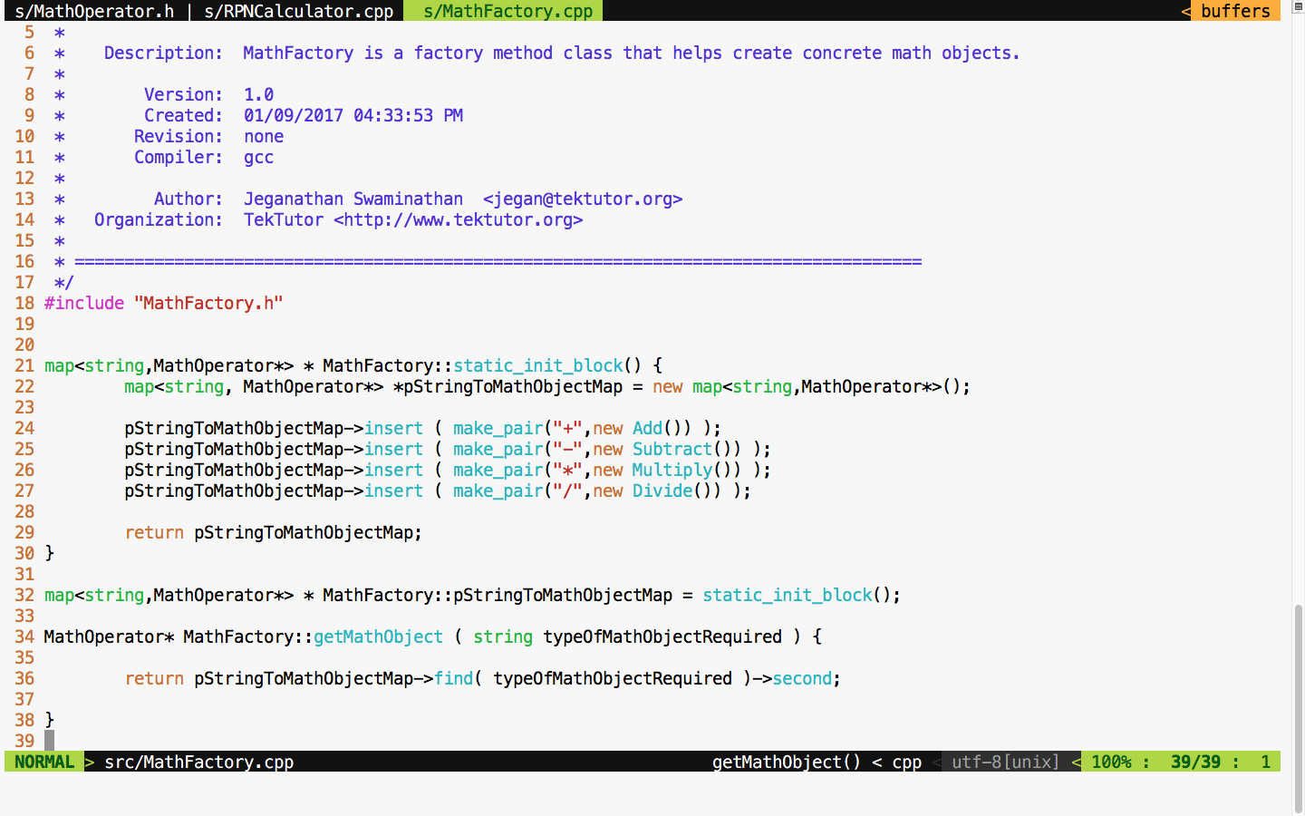
As much as possible, we must strive to avoid if-else conditions, or in general, we must try to avoid code branching when possible. Hence, STL map is used to avoid if-else conditions. This also promotes the reuse of the same Math objects, irrespective of the complexity of the RPN expression.
You will get an idea of how the MathOperator Add class is implemented if you refer to Figure 7.38:
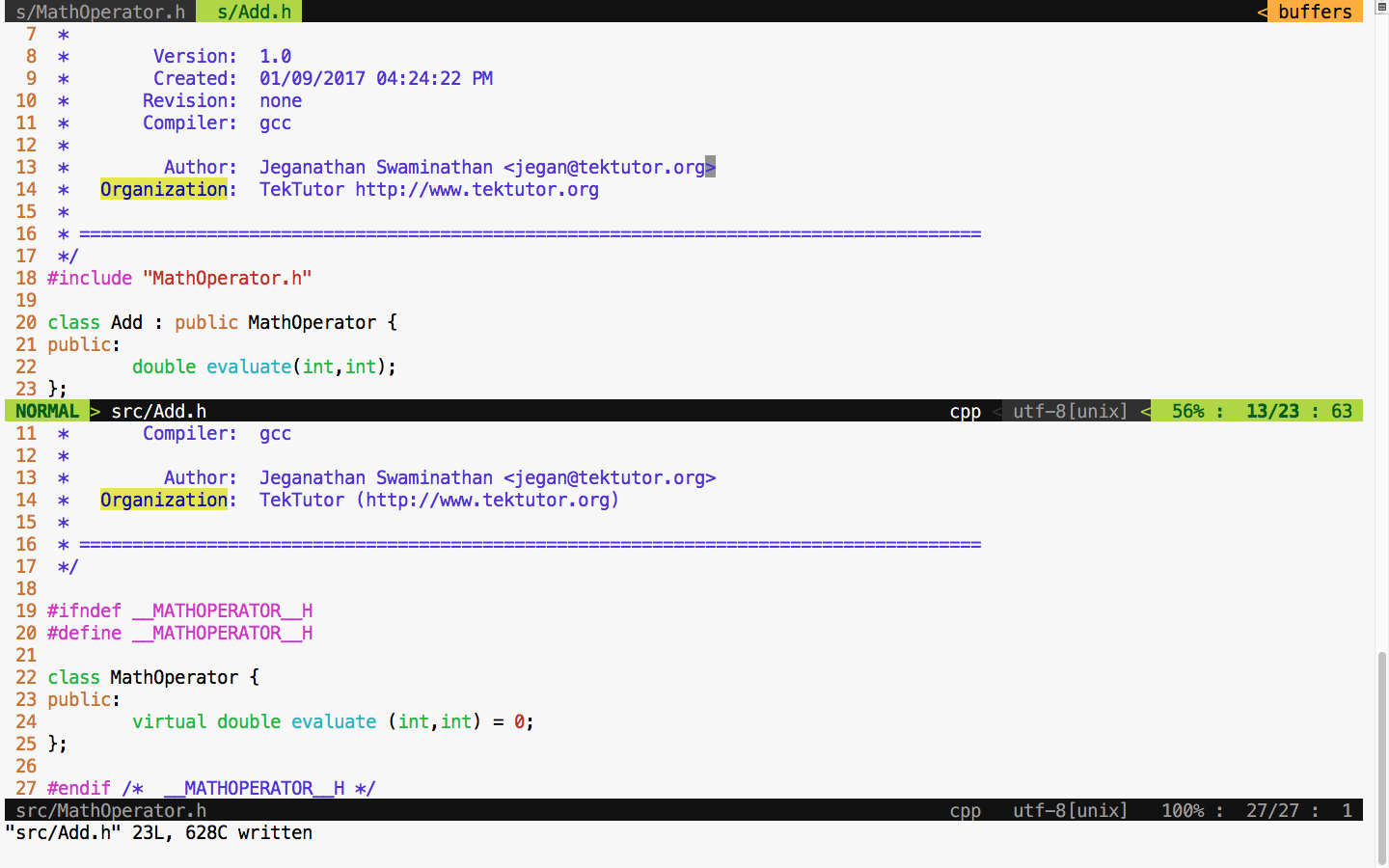
The Add class definition looks as shown in Figure 7.39:
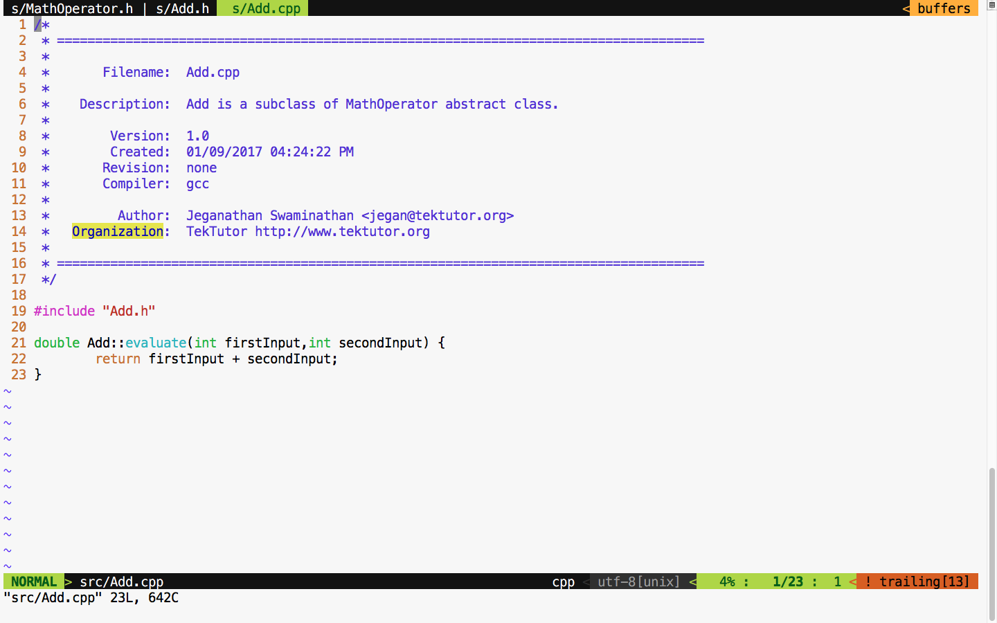
The subtract, multiplication, and division classes can be implemented in the similar fashion, as an Add class. The bottom line is that after refactoring, we can refactor a single RPNCalculator class into smaller and maintainable classes that can be tested individually.
Let's take a look at the refactored Makefile class in Figure 7.40 and test our code after the refactoring process is complete:
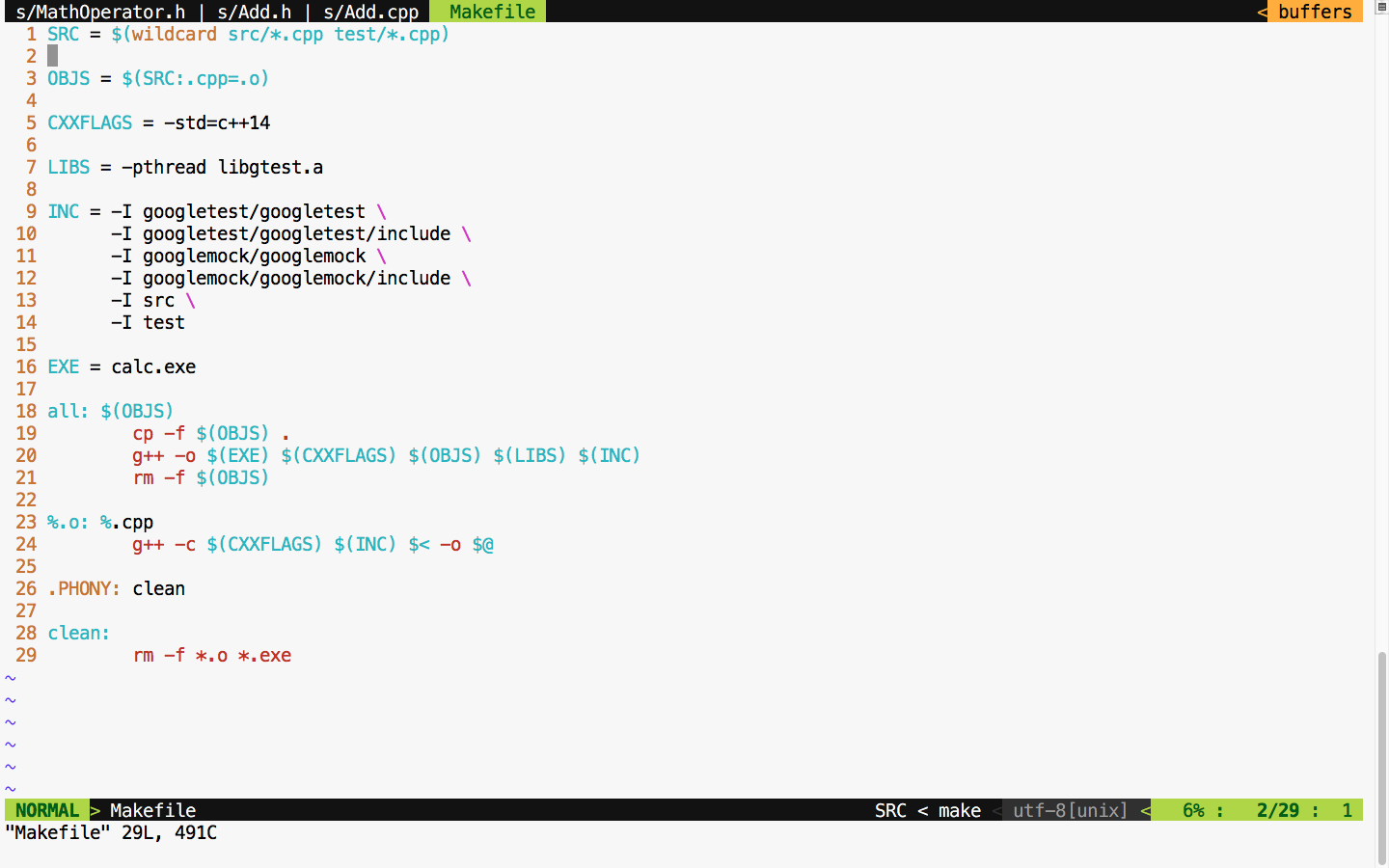
If all goes well, we should see all the test cases pass after refactoring if no functionalities are broken, as shown in Figure 7.41:
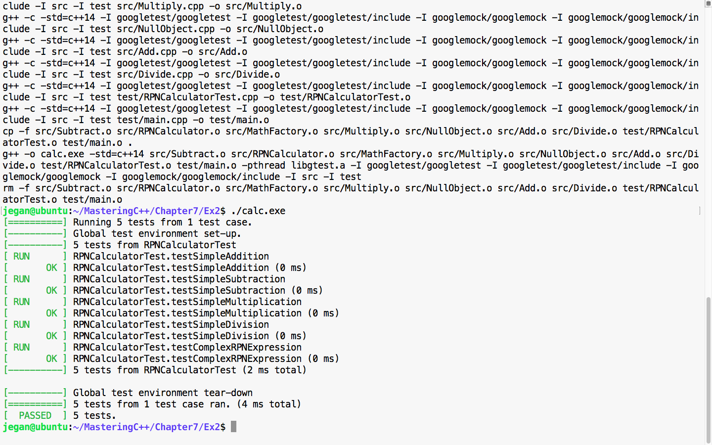
Cool! All the test cases have passed, hence it is guaranteed that we haven't broken the functionality in the process of refactoring. The main intent of TDD is to write testable code that is both functionally and structurally clean.
In the previous section, the CUT was independent with no dependency, hence the way it tested the code was straightforward. However, let's discuss how we can unit test the CUT that has dependencies. For this, refer to the following image:
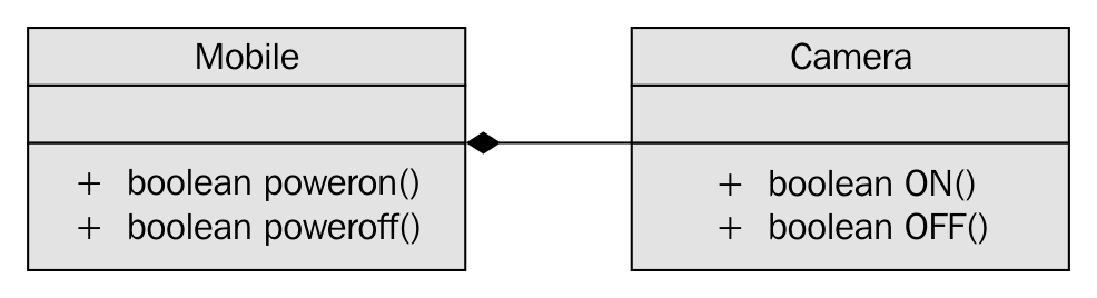
In Figure 7.42, it is apparent that Mobile has a dependency on Camera and the association between Mobile and Camera is composition. Let's see how the Camera.h header file is implemented in a legacy application:
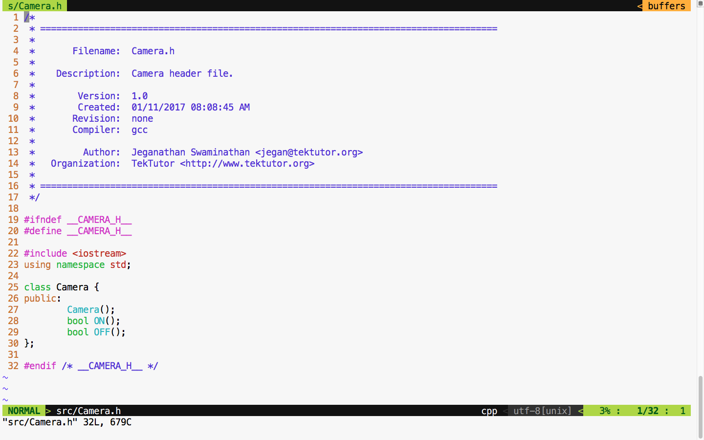
For demonstration purposes, let's take this simple Camera class that has ON() and OFF() functionalities. Let's assume that the ON/OFF functionality will interact with the camera hardware internally. Check out the Camera.cpp source file in Figure 7.44:
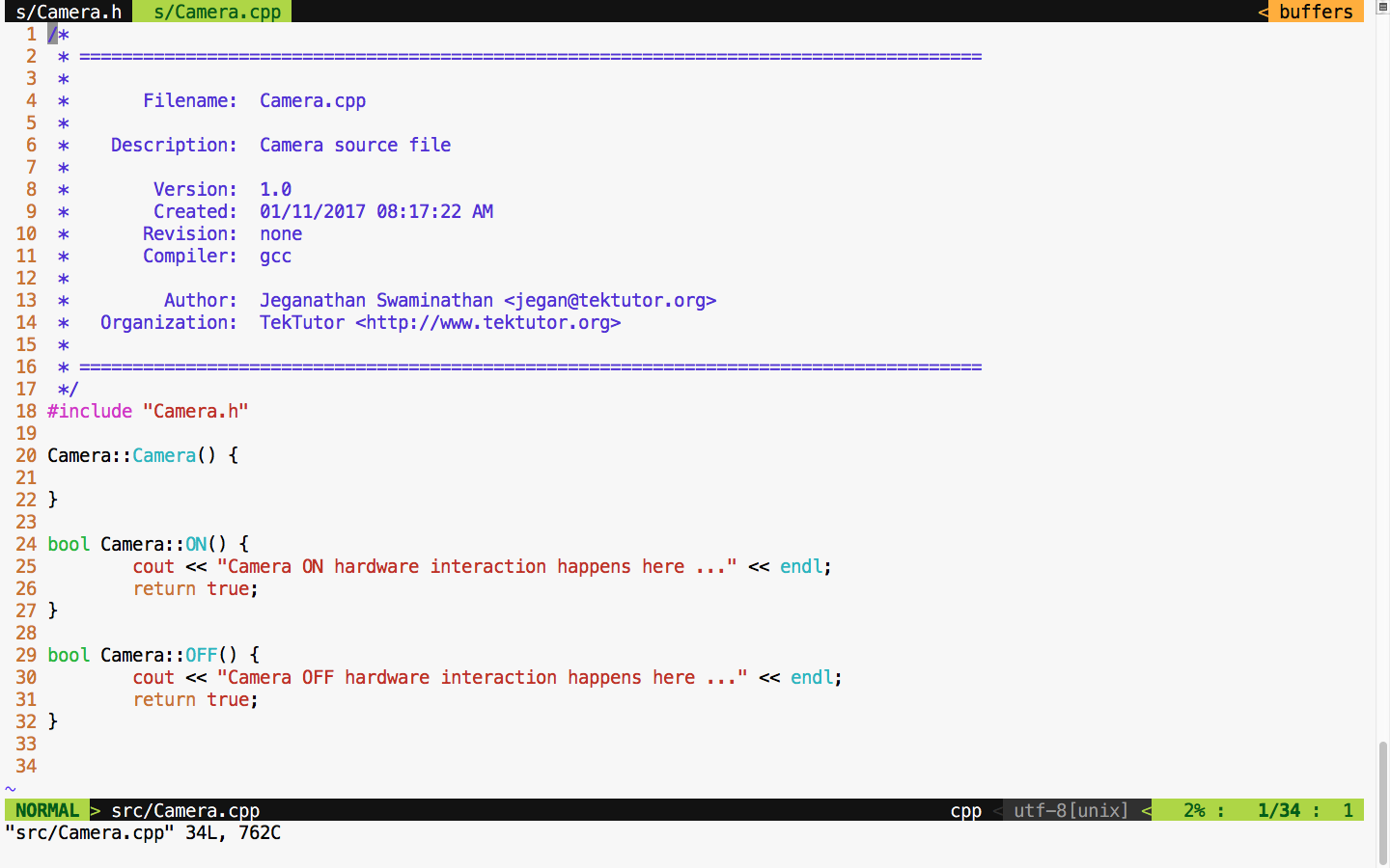
For debugging purposes, I have added some print statements that will come in handy when we test the powerOn() and powerOff() functionalities of mobile. Now let's check the Mobile class header file in Figure 7.45:
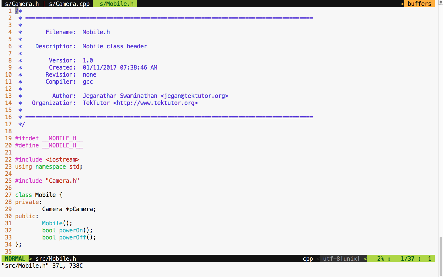
We move on to the mobile implementation, as illustrated in Figure 7.46:
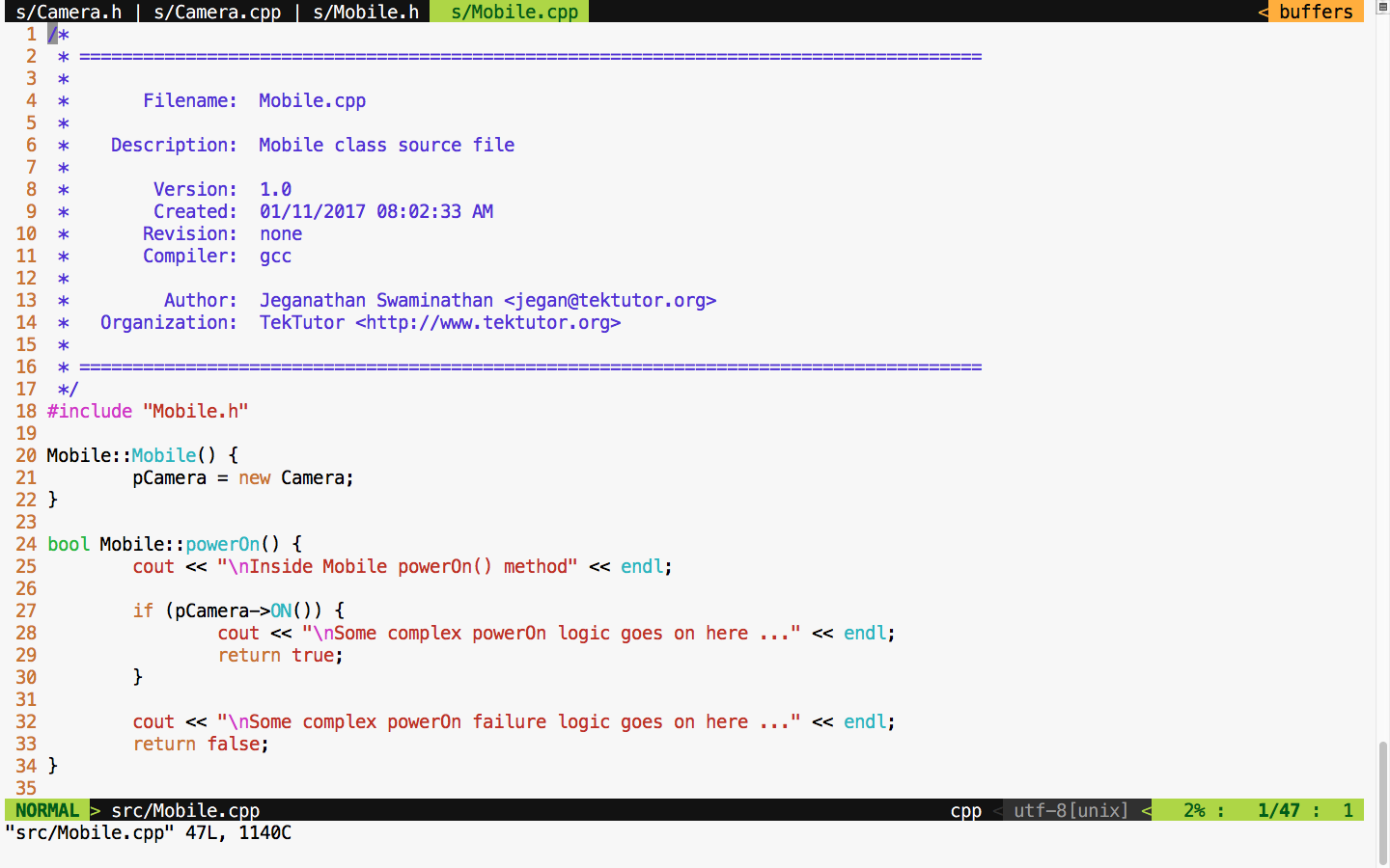
From the Mobile constructor implementation, it is evident that mobile has a camera or to be precise composition relationship. In other words, the Mobile class is the one that constructs the Camera object, as shown in Figure 7.46, line 21, in the constructor. Let's try to see the complexity involved in testing the powerOn() functionality of Mobile; the dependency has a composition relationship with the CUT of Mobile.
Let's write the powerOn() test case assuming camera On has succeeded, as follows:
TEST ( MobileTest, testPowerOnWhenCameraONSucceeds ) {

     Mobile mobile;
     ASSERT_TRUE ( mobile.powerOn() );

}
Now let's try to run the Mobile test case and check the test outcome, as illustrated in Figure 7.47:
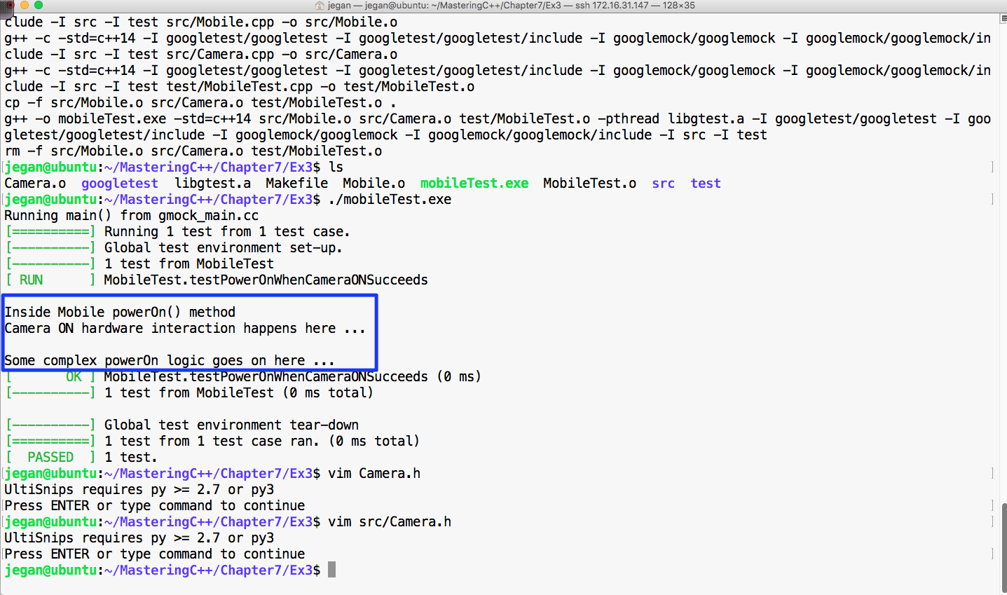
From Figure 7.47, we can understand that the powerOn() test case of Mobile has passed. However, we also understand that the real ON() method of the Camera class also got invoked. This, in turn, will interact with the camera hardware. At the end of the day, it is not a unit test as the test outcome isn't completely dependent on the CUT. If the test case had failed, we wouldn't have been able to pinpoint whether the failure was due to the code in the powerOn() logic of mobile or the code in the ON() logic of camera, which would have defeated the purpose of our test case. An ideal unit test should isolate the CUT from its dependencies using dependency injection and test the code. This approach will help us identify the behavior of the CUT in normal or abnormal scenarios. Ideally, when a unit test case fails, we should be able to guess the root cause of the failure without debugging the code; this is only possible when we manage to isolate the dependencies of our CUT.
The key benefit of this approach is that the CUT can be tested even before the dependency is implemented, which helps test 60~70 percent of the code without the dependencies. This naturally reduces the time to market the software product.
This is where the Google mock or gmock comes in handy. Let's check how we can refactor our code to enable dependency injection. Though it sounds very complex, the effort required to refactor code isn't that complex. In reality, the effort required to refactor your production code could be more complex, but it is worth the effort. Let's take a look at the refactored Mobile class shown in Figure 7.48:
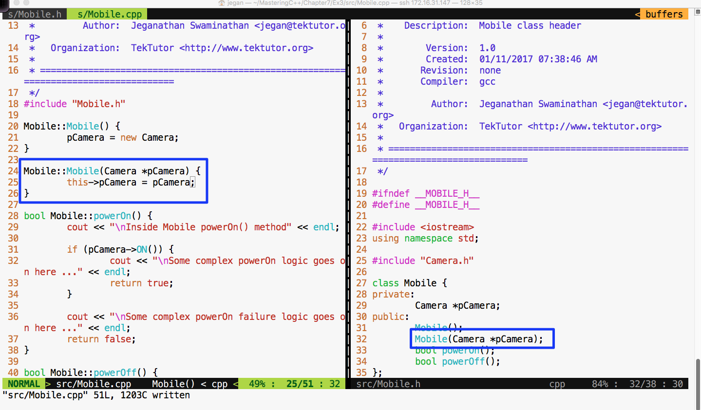
In the Mobile class, I have added an overloaded constructor that takes camera as an argument. This technique is called constructor dependency injection. Let's see how this simple yet powerful technique could help us isolate the camera dependency while testing the powerOn() functionality of Mobile.
Also, we must refactor the Camera.h header file and declare the ON() and OFF() methods as virtual in order for the gmock framework to help us stub these methods, as shown in Figure 7.49:
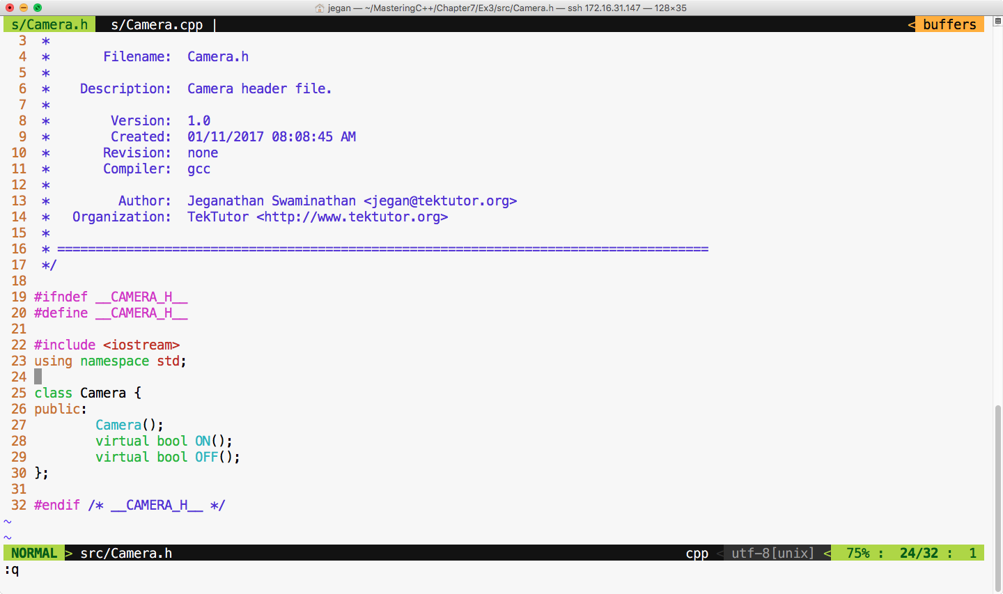
Now let's refactor our test case as shown in Figure 7.50:
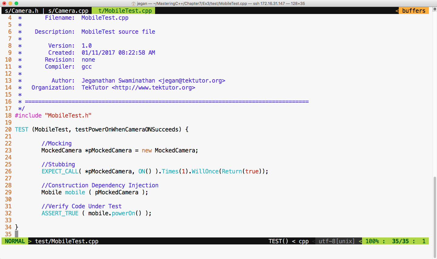
We are all set to build and execute the test cases. The test outcome is expected as shown in Figure 7.51:
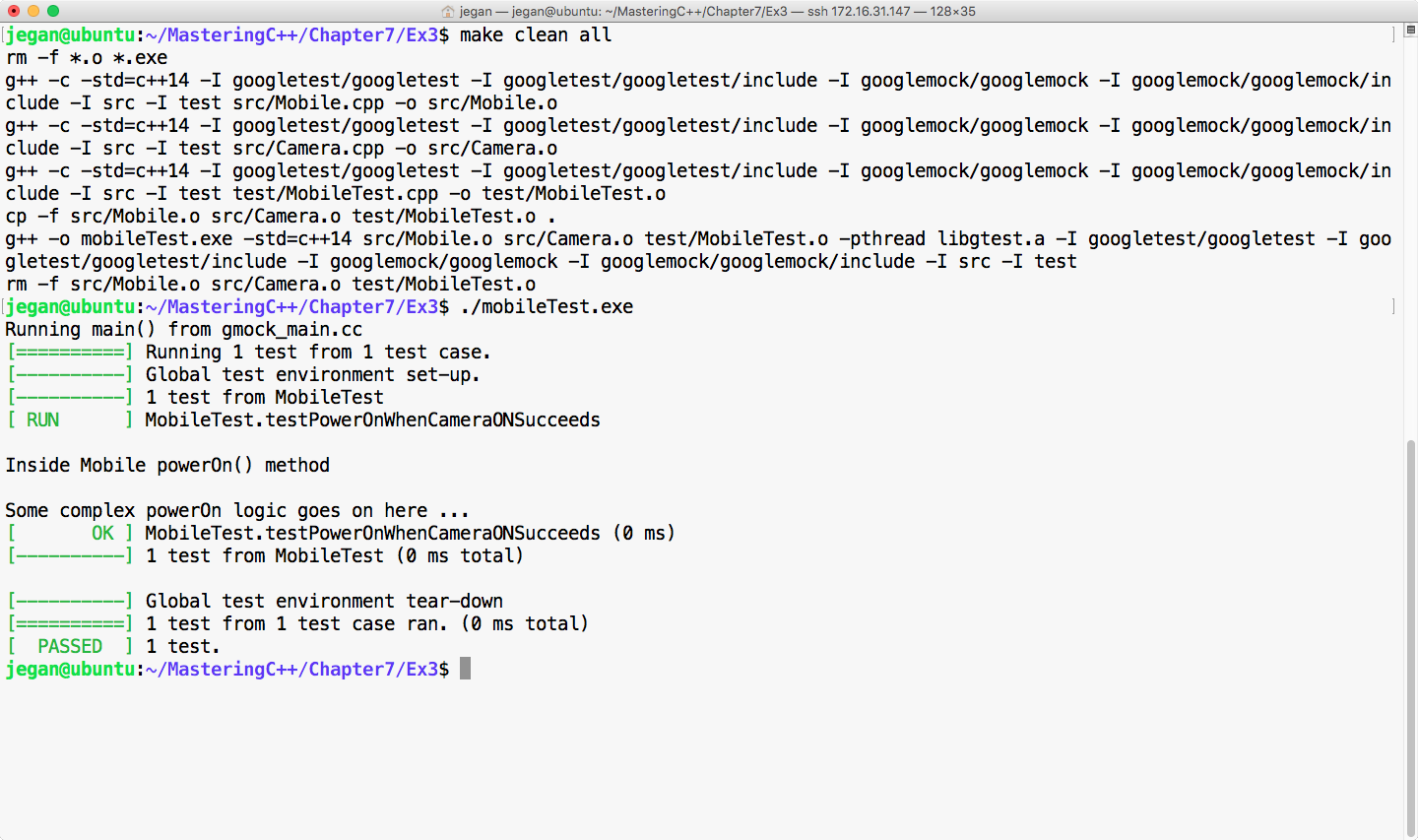
Cool! Not only has our test case passed, but we have also isolated our CUT from its camera dependency, which is evident as we don't see the print statements from the ON() method of camera. The bottom line is you have now learned how to unit test code by isolating its dependencies.
Happy TDD!
In this chapter, you learned quite a lot about TDD, and the following is the summary of the key takeaway points:
You have learned TDD and how to automate Unit Test Cases, Integration Test Cases, and Interaction Test cases in a bottom-up approach. With BDD, you will learn the top-down development approach, writing end-to-end functionalities and test cases and other complex test scenarios that we did not cover while discussing TDD.
In the next chapter, you will learn about Behavior-Driven Development.
This chapter covers the following topics:
In the following sections, let's look into each topic with easy-to-digest and interesting code samples in a practical fashion.
Behavior-driven development (BDD) is an outside-in development technique. BDD encourages capturing the requirements as a set of scenarios or use cases that describe how the end user will use the feature. The scenario will precisely express what will be the input supplied and what is the expected response from the feature. The best part of BDD is that it uses a domain-specific language (DSL) called Gherkin to describe the BDD scenarios.
Gherkin is an English-like language that is used by all the BDD test frameworks. Gherkin is a business-readable DSL that helps you describe the test case scenarios, keeping out the implementation details. The Gherkin language keywords are a bunch of English words; hence the scenarios can be understood by both technical and non-technical members involved in a software product or a project team.
Did I tell you that the BDD scenarios written in Gherkin languages serve as both documentation and test cases? As the Gherkin language is easy to understand and uses English-like keywords, the product requirements can be directly captured as BDD scenarios, as opposed to boring Word or PDF documents. Based on my consulting and industry experience, I have observed that a majority of the companies never update the requirement documents when the design gets refactored in the due course of time. This leads to stale and non-updated documents, which the development team will not trust for their reference purposes. Hence, the effort that has gone towards preparing the requirements, high-level design documents, and low-level design documents goes to waste in the long run, whereas Cucumber test cases will stay updated and relevant at all times.
TDD is an inside-out development technique whereas BDD is an outside-in development technique. TDD mainly focuses on unit testing and integration test case automation.
BDD focuses on end-to-end functional test cases and user acceptance test cases. However, BDD could also be used for unit testing, smoke testing, and, literally, every type of testing.
BDD is an extension of the TDD approach; hence, BDD also strongly encourages test-first development. It is quite natural to use both BDD and TDD in the same product; hence, BDD isn't a replacement for TDD. BDD can be thought of as a high-level design document, while TDD is the low-level design document.
In C++, TDD test cases are written using testing frameworks such as CppUnit, gtest, and so on, which require a technical background to understand them and hence, are generally used only by developers.
In C++, BDD test cases are written using a popular test framework called cucumber-cpp. The cucumber-cpp framework expects that the test cases are written in the Gherkin language, while the actual test case implementations can be done with any test framework, such as gtest or CppUnit.
However, in this book, we will be using cucumber-cpp with the gtest framework.
Gherkin is the universal language used by every BDD framework for various programming languages that enjoy BDD support.
Gherkin is a line-oriented language, similar to YAML or Python. Gherkin will interpret the structure of the test case based on indentations.
The # character is used for a single line of comment in Gherkin. At the time of writing this book, Gherkin support about 60 keywords.
Gherkin is a DSL used by the Cucumber framework.
Installing the cucumber-cpp framework is quite straightforward in Linux. All you need to do is either download or clone the latest copy of cucumber-cpp.
The following command can be used to clone the cucumber-cpp framework:
git clone https://github.com/cucumber/cucumber-cpp.git
The cucumber-cpp framework is supported in Linux, Windows, and Macintosh. It can be integrated with Visual Studio on Windows or Xcode on macOS.
The following screenshot demonstrates the Git clone procedure:
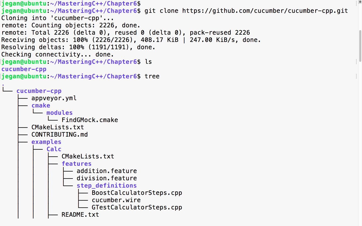
As cucumber-cpp depends on a wire protocol to allow the writing of BDD test case step definitions in the C++ language, we need to install Ruby.
The following command helps you install Ruby on your Ubuntu system. This is one of the prerequisite software that is required for the cucumber-cpp framework:
sudo apt install ruby
The following screenshot demonstrates the Ruby installation procedure:
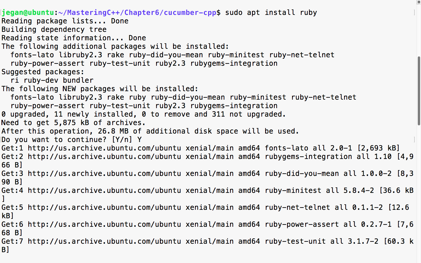
Once the installation is complete, please ensure that Ruby is installed properly by checking its version. The following command should print the version of Ruby installed on your system:
ruby --version
In order to complete the Ruby installation, we need to install the ruby-dev packages, as follows:
sudo apt install ruby-dev
Next, we need to ensure that the bundler tool is installed so that the Ruby dependencies are installed by the bundler tool seamlessly:
sudo gem install bundler
bundle install
If it all went smooth, you can go ahead and check if the correct version of Cucumber, Ruby, and Ruby's tools are installed properly. The bundle install command will ensure that Cucumber and other Ruby dependencies are installed. Make sure you don't install bundle install as a sudo user; this will prevent non-root from accessing the Ruby gem packages:
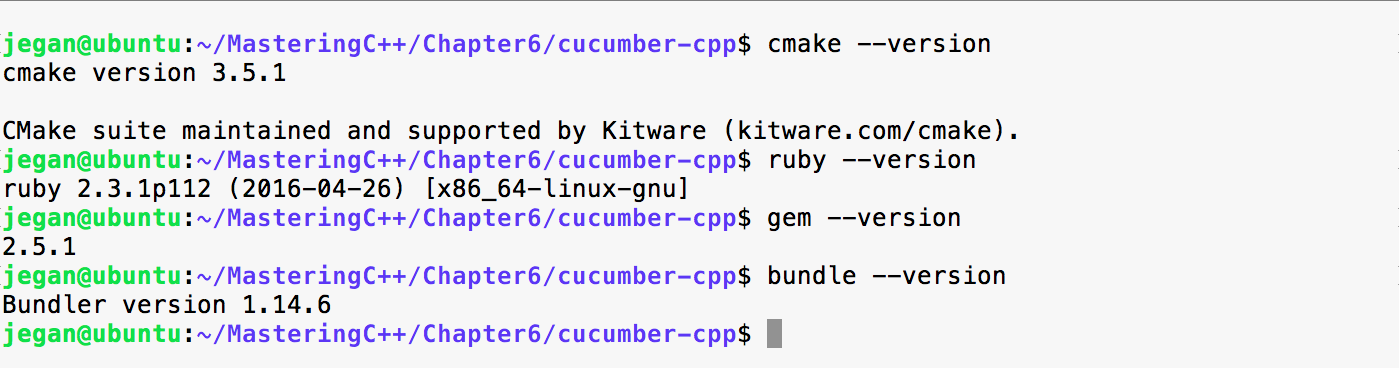
We are almost done, but we are not there yet. We need to build the cucumber-cpp project; as part of that, let's get the latest test suite for the cucumber-cpp framework:
git submodule init
git submodule update
We go on to install the ninja and boost libraries before we can initiate the build. Though we aren't going to use the boost test framework in this chapter, the travis.sh script file looks for the boost library. Hence, I would suggest installing the boost library in general, as part of Cucumber:
sudo apt install ninja-build
sudo apt-get install libboost-all-dev
Now, it's time to build the cucumber-cpp framework. Let's create the build folder. In the cucumber-cpp folder, there will be a shell script by the name, travis.sh. You got to execute the script to build and execute the test cases:
sudo ./travis.sh
Though the previous approach works, my personal preference and recommendation would be the following approach. The reason behind recommending the following approach is that the build folder is supposed to be created as a non-root user, as anyone should be able to perform the build once the cucumber-cpp setup is complete. You should be able to find the instructions in the README.md file under the cucumber-cpp folder:
git submodule init
git submodule update
cmake -E make_directory build
cmake -E chdir build cmake --DCUKE_ENABLE_EXAMPLES=on ..
cmake --build build
cmake --build build --target test
cmake --build build --target features
If you were able to complete all the previous installation steps exactly as explained, you are all set to start playing with cucumber-cpp. Congrats!!!
Every product feature will have a dedicated feature file. The feature file is a text file with the .feature extension. A feature file can contain any number of scenarios, and each scenario is equivalent to a test case.
Let's take a look at a simple feature file example:
1   # language: en
2
3   Feature: The Facebook application should authenticate user login.
4
5     Scenario: Successful Login
6        Given I navigate to Facebook login page https://www.facebook.com
7        And I type jegan@tektutor.org as Email
8        And I type mysecretpassword as Password
9        When I click the Login button
10       Then I expect Facebook Home Page after Successful Login
Cool, it appears like plain English, right? But trust me, this is how Cucumber test cases are written! I understand your doubt--it looks easy and cool but how does this verify the functionality, and where is the code that verifies the functionality? The cucumber-cpp framework is a cool framework, but it doesn't natively support any testing functionalities; hence cucumber-cpp depends on the gtest, CppUnit, other test frameworks. The test case implementation is written in a Steps file, which can be written in C++ using the gtest framework in our case. However, any test framework will work.
Every feature file will start with the Feature keyword followed by one or more lines of description that describe the feature briefly. In the feature file, the words Feature, Scenario, Given, And, When, and Then are all Gherkin keywords.
A feature file may contain any number of scenarios (test cases) for a feature. For instance, in our case, login is the feature, and there could be multiple login scenarios as follows:
Every line following the scenario will translate into one function in the Steps_definition.cpp source file. Basically, the cucumber-cpp framework maps the feature file steps with a corresponding function in the Steps_definition.cpp file using regular expressions.
Gherkin supports over 60 spoken languages. As a best practice, the first line of a feature file will indicate to the Cucumber framework that we would like to use English:
1 # language: en
The following command will list all the spoken languages supported by the cucumber-cpp framework:
cucumber -i18n help
The list is as follows:
Like TDD, the Cucumber framework too recommends a project folder structure. The recommended cucumber-cpp project folder structure is as follows:
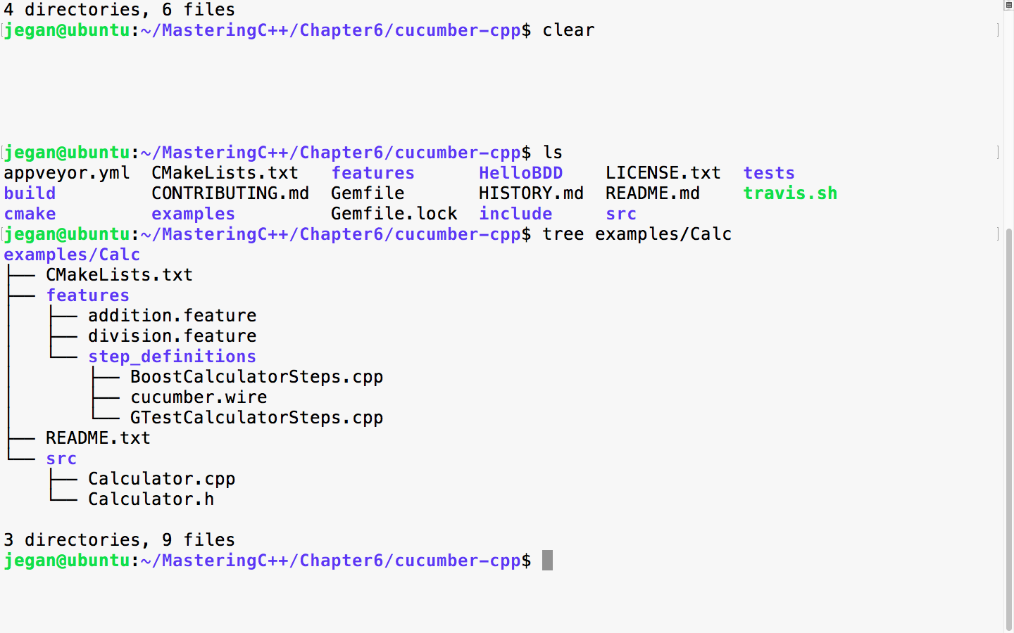
The src folder will contain the production code, that is, all your project files will be maintained under the src directory. The BDD feature files will be maintained under the features folder and its respective Steps file, which has either boost test cases or gtest cases. In this chapter, we will be using the gtest framework with cucumber-cpp. The wire file has wire protocol-related connection details such as the port and others. The CMakeLists.txt is the build script that has the instructions to build your project along with its dependency details, just like Makefile used by the MakeBuild utility.
Let's write our very first Cucumber test case! As this is our first exercise, I would like to keep it short and simple. First, let's create the folder structure for our HelloBDD project.
To create the Cucumber project folder structure, we can use the cucumber utility, as follows:
cucumber --init
This will ensure that the features and steps_definitions folders are created as per Cucumber best practices:
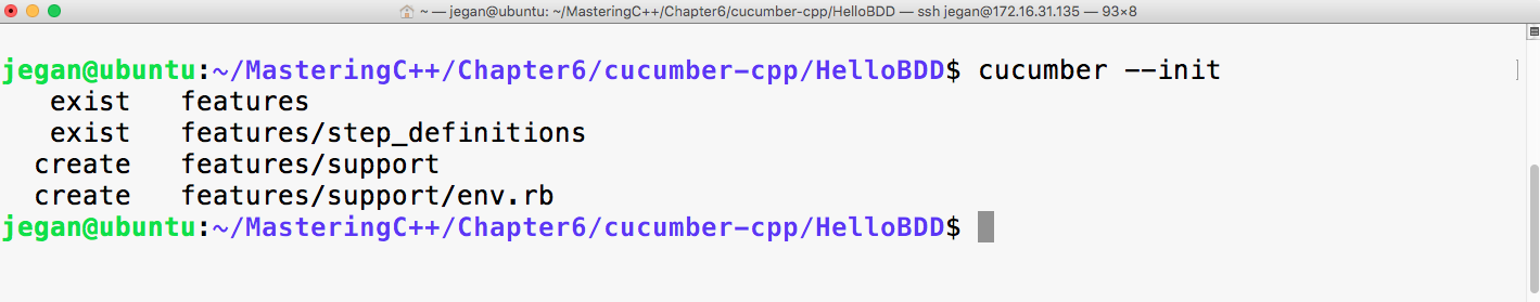
Once the basic folder structure is created, let's manually create the rest of the files:
mkdir src
cd HelloBDD
touch CMakeLists.txt
touch features/hello.feature
touch features/step_definitions/cucumber.wire
touch features/step_definitions/HelloBDDSteps.cpp
touch src/Hello.h
touch src/Hello.cpp
Once the folder structure and empty files are created, the project folder structure should look like the following screenshot:
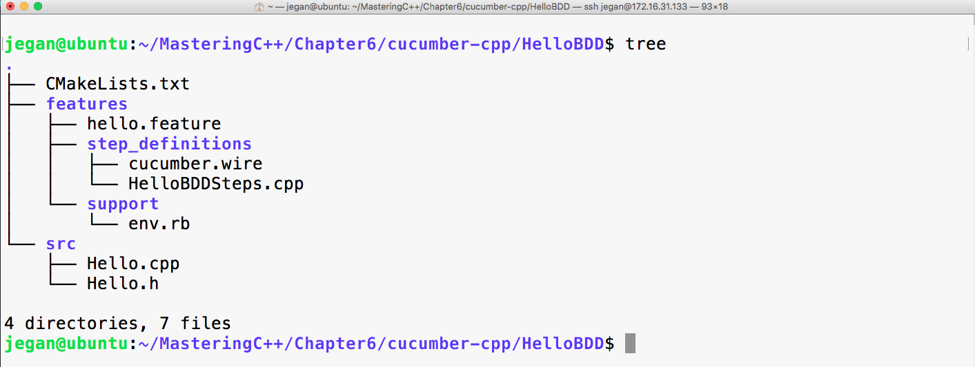
It's time to start applying our Gherkin knowledge in action; hence, let's first start with the feature file:
# language: en

Feature: Application should be able to print greeting message Hello BDD!

   Scenario: Should be able to greet with Hello BDD! message
      Given an instance of Hello class is created
      When the sayHello method is invoked
      Then it should return "Hello BDD!"
Let's take a look at the cucumber.wire file:
host: localhost
port: 3902
Now let's see how to write the steps file using the gtest Framework.
You can observe the written steps files using gtest in the following screenshot:
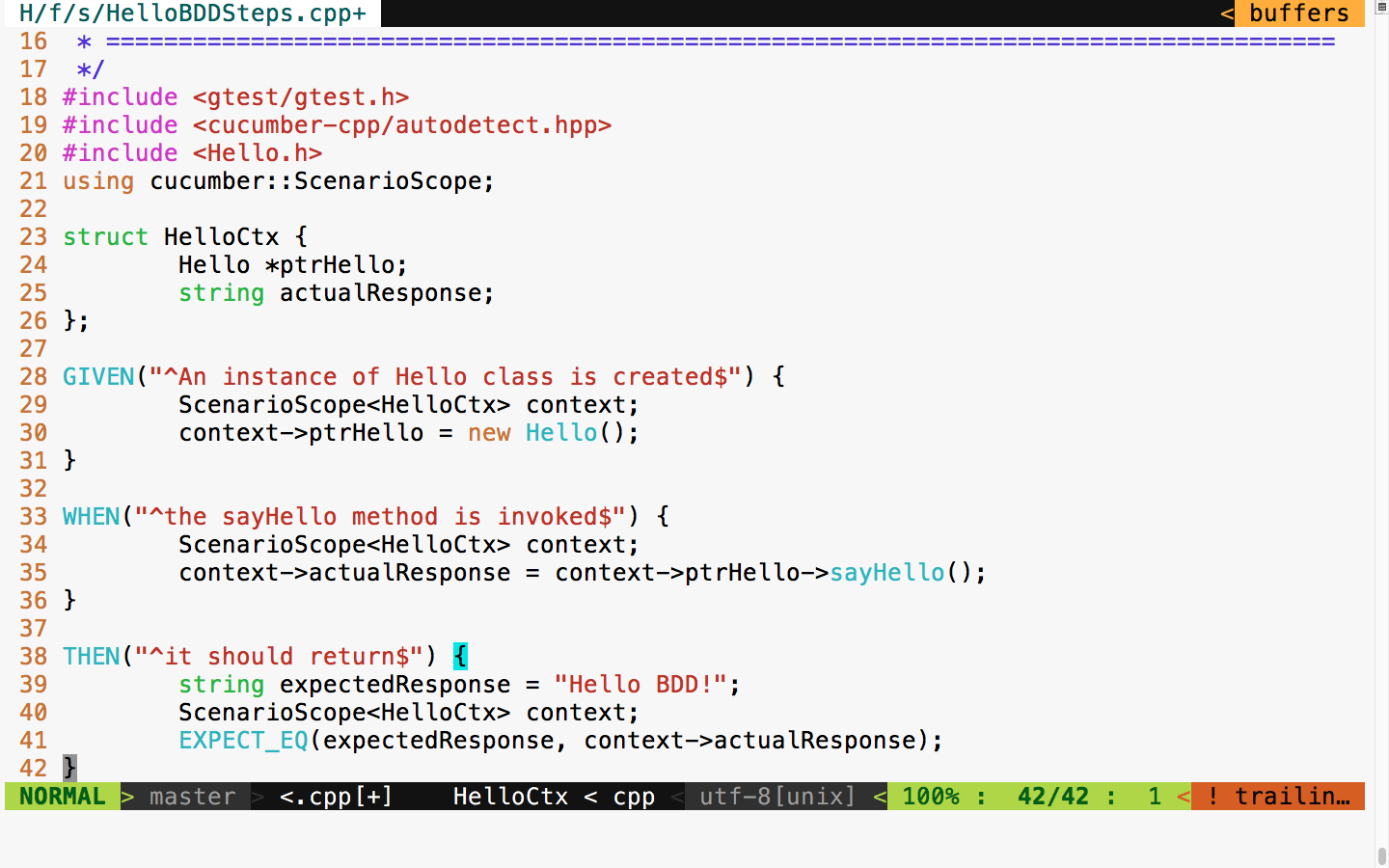
The following header files ensure that the gtest header and Cucumber headers necessary for writing Cucumber steps are included:
#include <gtest/gtest.h>
#include <cucumber-cpp/autodetect.hpp>
Now let's proceed with writing the steps:
struct HelloCtx {
     Hello *ptrHello;
     string actualResponse;
};
The HelloCtx struct is a user-defined test context that holds the object instance under test and its test response. The cucumber-cpp framework offers a smart ScenarioScope class that allows us to access the object under test and its output, across all the steps in a Cucumber test scenario.
For every Given, When, and Then statement that we wrote in the feature file, there is a corresponding function in the steps file. The appropriate cpp functions that correspond to Given, When, and Then are mapped with the help of regular expressions.
For instance, consider the following Given line in the feature file:
Given an instance of Hello class is created
This corresponds to the following cpp function that gets mapped with the help of regex. The ^ character in the regex implies that the pattern starts with an, and the $ character implies that the pattern ends with created:
GIVEN("^an instance of Hello class is created$")
{
       ScenarioScope<HelloCtx> context;
       context->ptrHello = new Hello();
}
As the GIVEN step says that, at this point, we must ensure that an instance of the Hello object is created; the corresponding C++ code is written in this function to instantiate an object of the Hello class.
On a similar note, the following When step and its corresponding cpp functions are mapped by cucumber-cpp:
When the sayHello method is invoked
It is important that the regex matches exactly; otherwise, the cucumber-cpp framework will report that it can't find the steps function:
WHEN("^the sayHello method is invoked$")
{
       ScenarioScope<HelloCtx> context;
       context->actualResponse = context->ptrHello->sayHello();
}
Now let's look at the Hello.h file:
#include <iostream>
#include <string>
using namespace std;

class Hello {
public:
       string sayHello();
};
Here is the respective source file, that is, Hello.cpp:
#include "Hello.h"

string Hello::sayHello() {
     return "Hello BDD!";
}
Finally, let's write CMakeLists.txt:
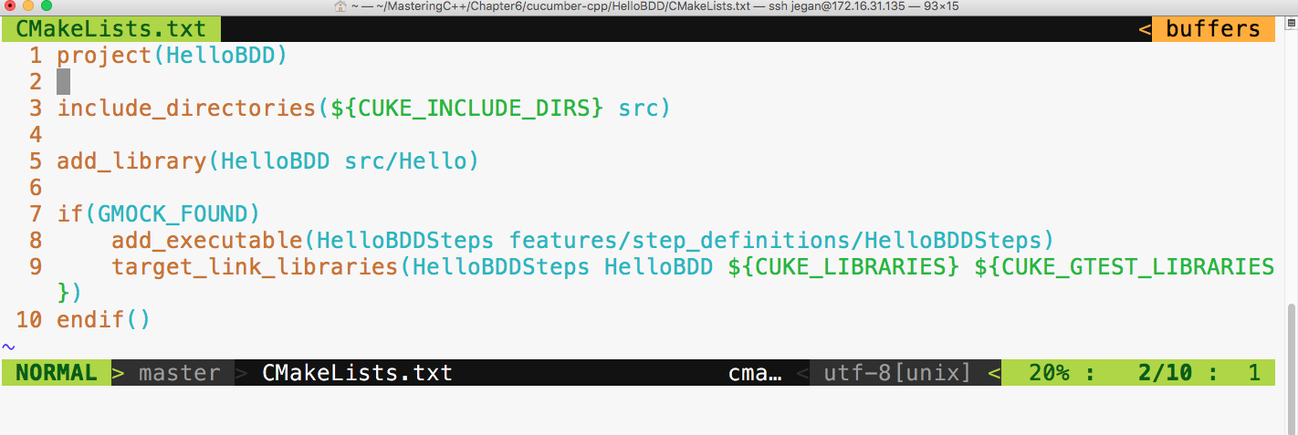
The first line implies the name of the project. The third line ensures that the Cucumber header directories and our project's include_directories are in the INCLUDE path. The fifth line basically instructs the cmake utility to create a library out of the files present under the src folder, that is, Hello.cpp, and its Hello.h file. The seventh line detects whether the gtest framework is installed on our system, and the eighth line ensures that the HelloBDDSteps.cpp file is compiled. Finally, in the ninth line, the final executable is created, linking all the HelloBDD libraries that have our production code, the HelloBDDSteps object file, and the respective Cucumber and gtest library files.
There is one last configuration that we need to do before we start building our project:
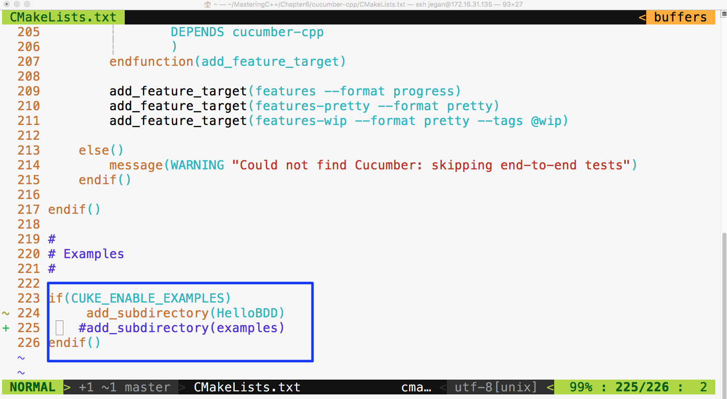
Basically, I have commented the examples subdirectories and added our HelloBDD project in CMakeLists.txt present under the cucumber-cpp folder, as shown earlier.
As we have created the project as per cucumber-cpp best practices, let's navigate to the HelloBDD project home and issue the following command:
cmake --build build
The following screenshot shows the build procedure:
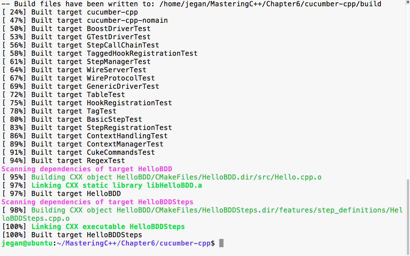
Now let's execute the test case. This involves two steps, as we are using the wire protocol. Let's first launch the test case executable in background mode and then Cucumber, as follows:
cmake --build build
build/HelloBDD/HelloBDDSteps > /dev/null &
cucumber HelloBDD
Redirecting to /dev/null isn't really mandatory. The main purpose of redirecting to a null device is to avoid distractions from the print statement that an application may spit in the terminal output. Hence, it is a personal preference. In case you prefer to see the debug or general print statements from your application, feel free to issue the command without redirection:
build/HelloBDD/HelloBDDSteps &
The following screenshot demonstrates the build and test execution procedure:
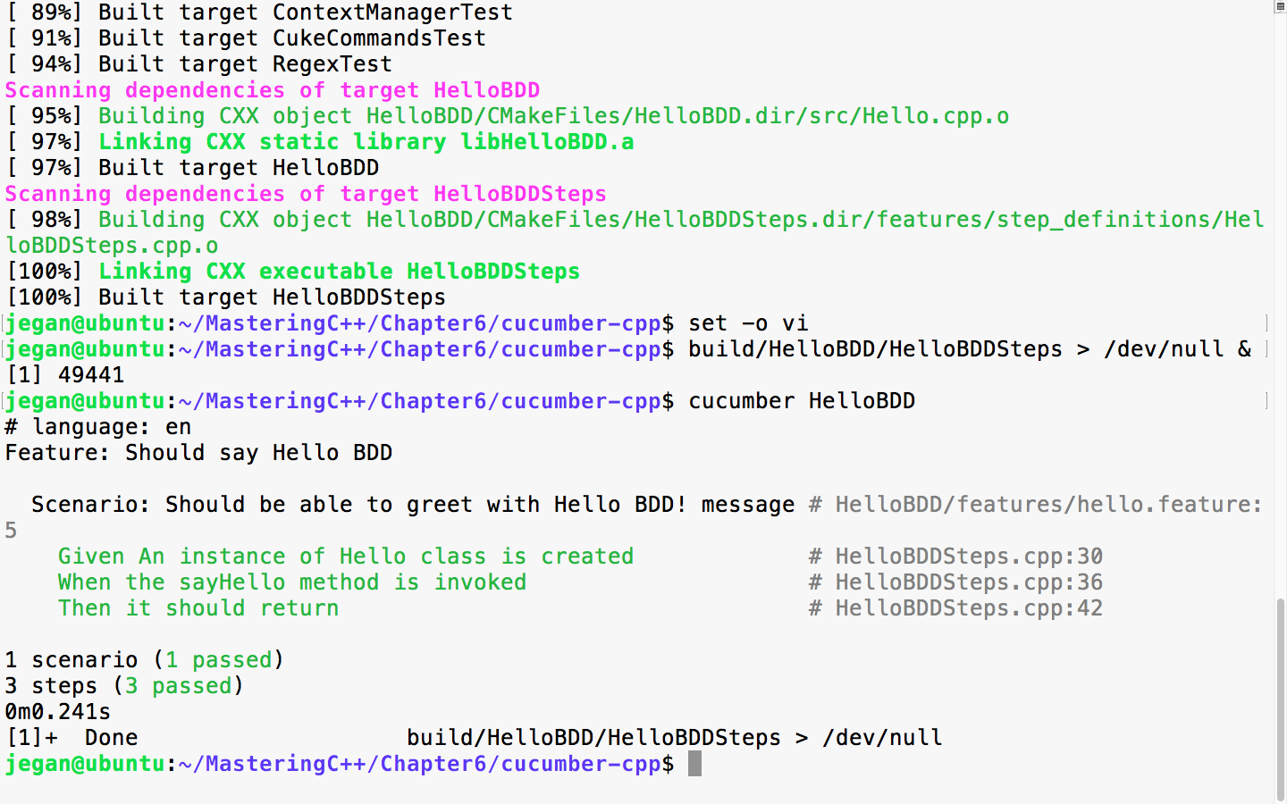
Congrats! our very first cucumber-cpp test case has passed. Each scenario represents a test case and the test case includes three steps; as all the steps passed, the scenario is reported as passed.
Do you want to quickly check whether the feature files and steps files are written correctly, without really executing them? Cucumber has a quick and cool feature to do so:
build/HelloBDD/HelloBDDSteps > /dev/null &
This command will execute our test application in the background mode. /dev/null is a null device in Linux OS, and we are redirecting all the unwanted print statements from the HelloBDDSteps executable to the null device to ensure it doesn't distract us while we execute our Cucumber test cases.
The next command will allow us to dry run the Cucumber test scenario:
cucumber --dry-run
The following screenshot shows the test execution:
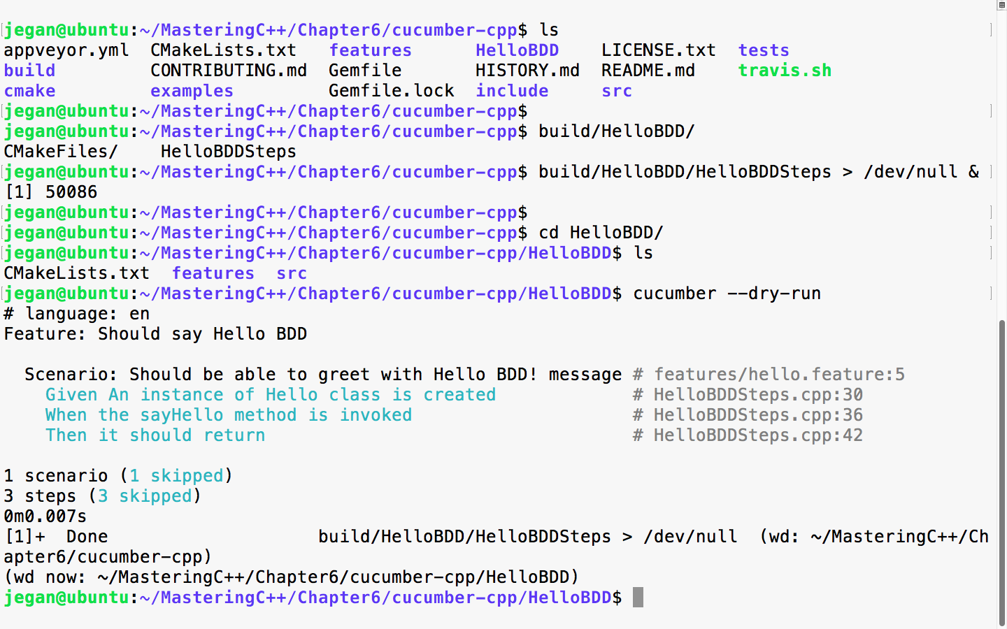
Just like TDD, BDD also insists on following a test-first development approach. Hence, in this section, let's explore how we could write an end-to-end feature following a test-first development approach the BDD way!
Let's take a simple example that helps us understand the BDD style of coding. We will write an RPNCalculator application that does addition, subtraction, multiplication, division, and complex math expressions that involve many math operations in the same input.
Let's create our project folder structure as per Cucumber standards:
mkdir RPNCalculator
cd RPNCalculator
cucumber --init
tree
mkdir src
tree
The following screenshot demonstrates the procedure visually:
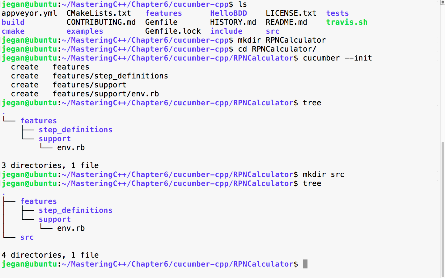
Great! The folder structure is now created. Now, let's create empty files with a touch utility to help us visualize our final project folder structure along with the files:
touch features/rpncalculator.feature
touch features/step_definitions/RPNCalculatorSteps.cpp
touch features/step_definitions/cucumber.wire
touch src/RPNCalculator.h
touch src/RPNCalculator.cpp
touch CMakeLists.txt
Once the dummy files are created, the final project folder structure will look like the following screenshot:
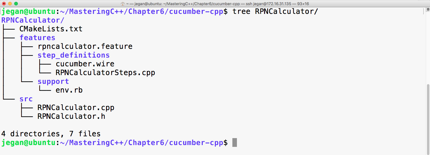
As usual, the Cucumber wire file is going to look as follows. In fact, throughout this chapter, this file will look same:
host: localhost
port: 3902
Now, let's start with the rpncalculator.feature file, as shown in the following screenshot:
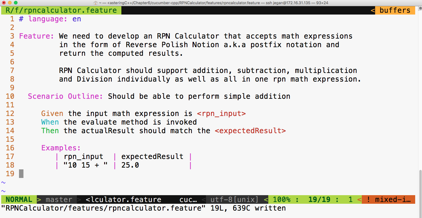
As you can see, the feature description can be pretty elaborate. Did you notice? I have used Scenario Outline in the place of scenario. The interesting part of Scenario Outline is that it allows describing the set of inputs and the corresponding output in the form of a table under the Examples Cucumber section.
We need to add our project in the CMakeLists.txt file at the cucumber-cpp home directory, as follows:
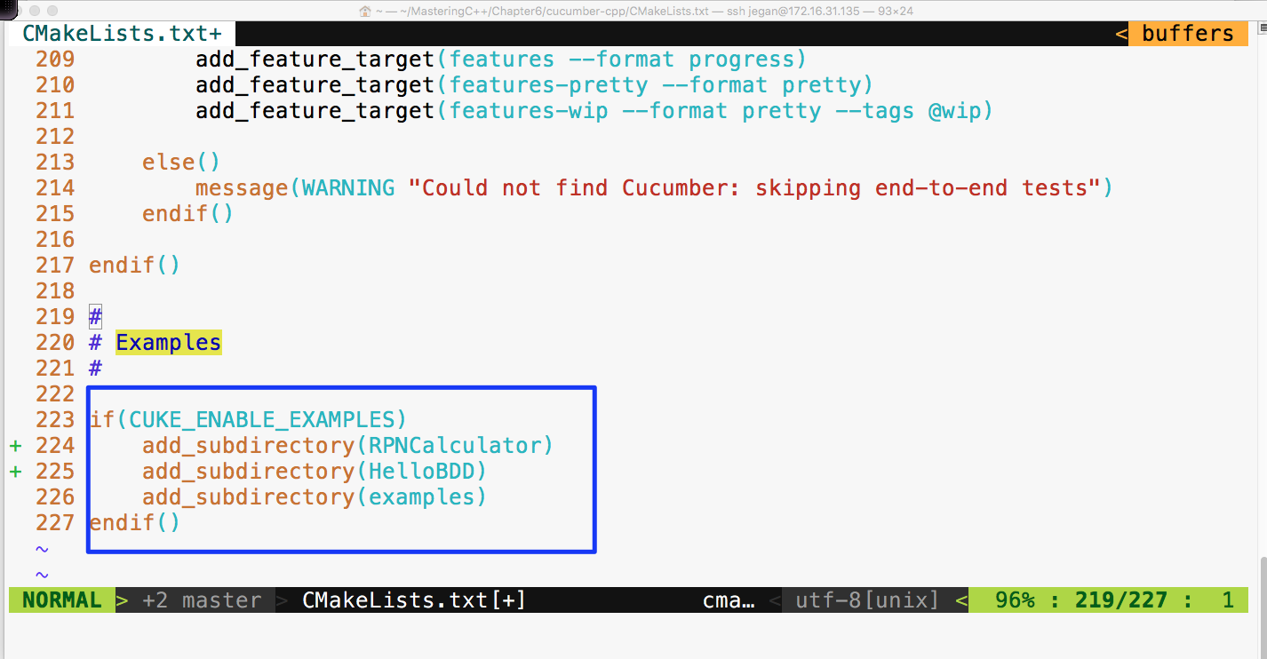
Ensure that CMakeLists.txt under the RPNCalculator folder looks as follows:
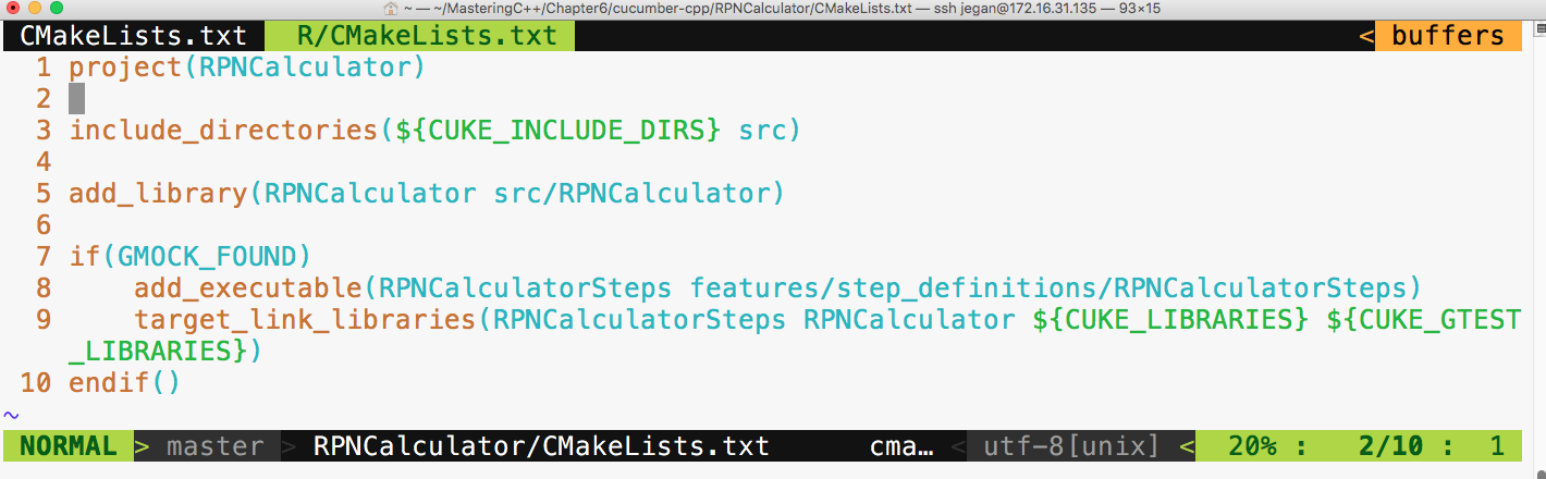
Now, let's build our project with the following command from the cucumber-cpp home directory:
cmake --build build
Let's execute our brand new RPNCalculator Cucumber test cases with the following command:
build/RPNCalculator/RPNCalculatorSteps &

cucumber RPNCalculator
The output looks as follows:
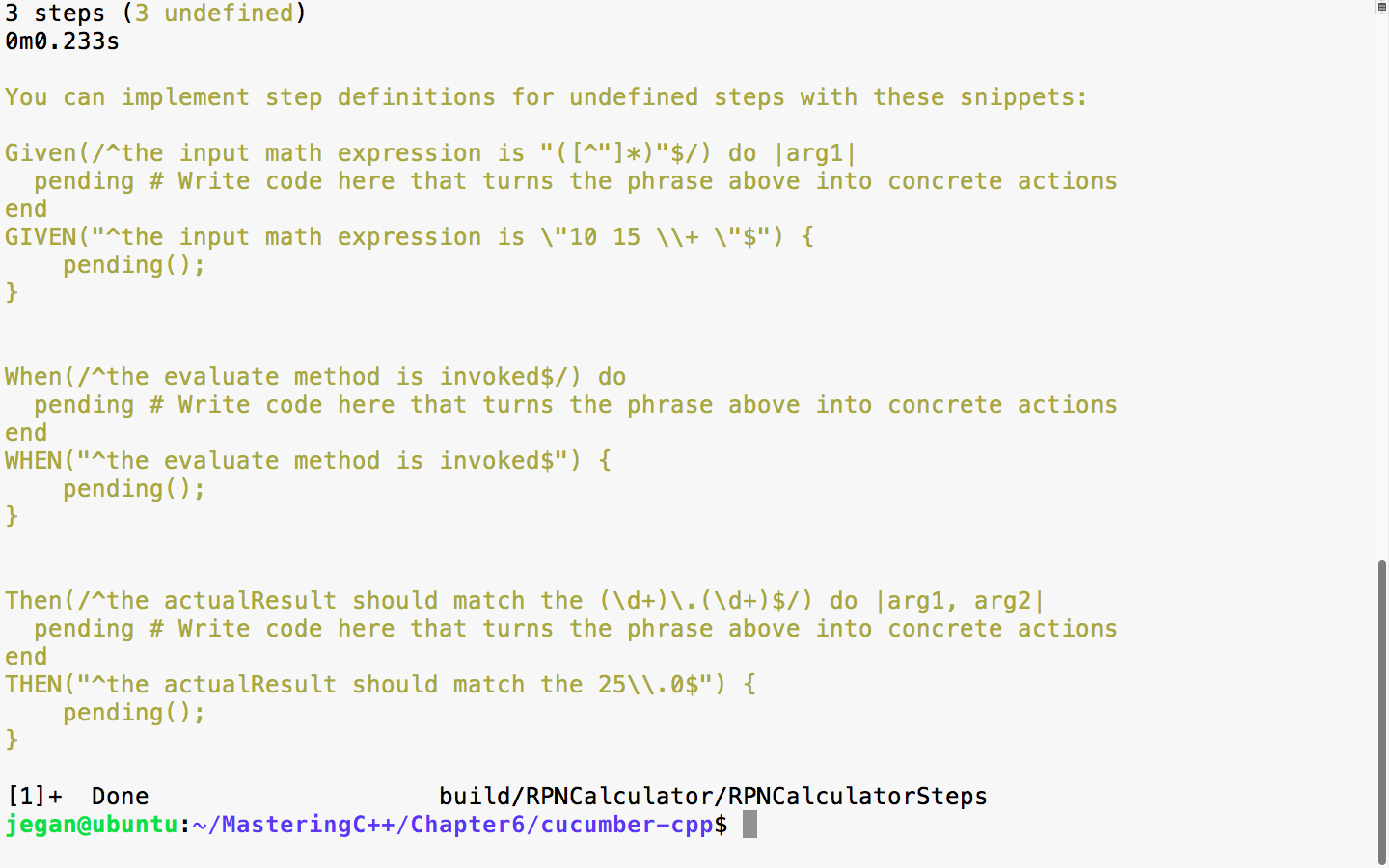
In the preceding screenshot, there are two suggestions for every Given, When, and Then statements we wrote in the feature file. The first version is meant for Ruby and the second is meant for C++; hence, we can safely ignore the step suggestions, which are as follows:
Then(/^the actualResult should match the (d+).(d+)$/) do |arg1, arg2|
   pending # Write code here that turns the phrase above into concrete actions
end
As we are yet to implement the RPNCalculatorSteps.cpp file, the Cucumber framework is suggesting us to supply implementations for the previous steps. Let's copy and paste them in the RPNCalculatorSteps.cpp file and complete the steps implementations, as follows:
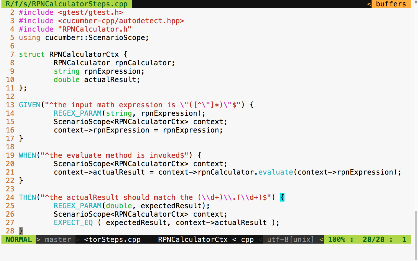
Now, let's try to build our project again with the following command:
cmake --build build
The build log looks as follows:
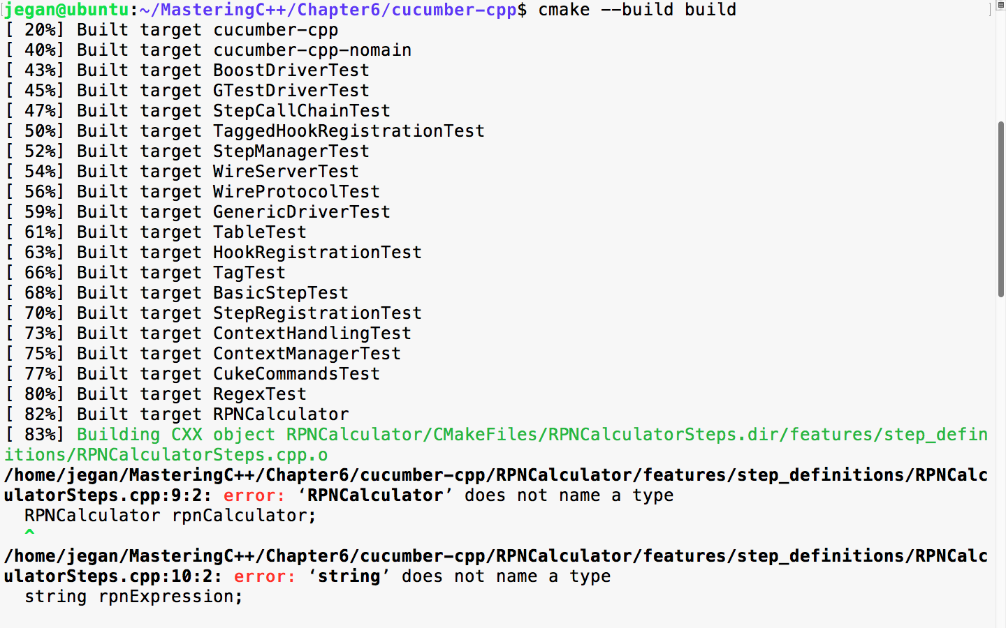
The secret formula behind every successful developer or consultant is that they have strong debugging and problem-solving skills. Analyzing build reports, especially build failures, is a key quality one should acquire to successfully apply BDD. Every build error teaches us something!
The build error is obvious, as we are yet to implement RPNCalculator, as the file is empty. Let's write minimal code such that the code compiles:
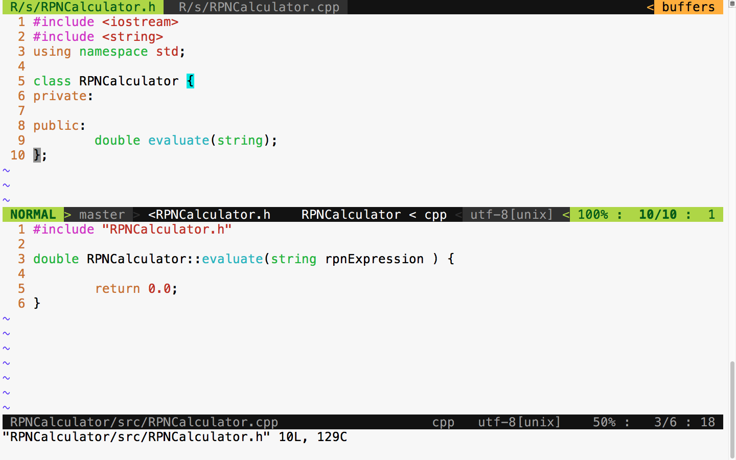
BDD leads to incremental design and development, unlike the waterfall model. The waterfall model encourages upfront design. Typically, in a waterfall model, the design is done initially, and it consumes 30-40% of the overall project effort. The main issue with upfront design is that we will have less knowledge about the feature initially; often, we will have a vague feature knowledge, but it will improve over time. So, it isn't a good idea to put in more effort in the design activity upfront; rather, be open to refactoring the design and code as and when necessary.
Hence, BDD is a natural choice for complex projects.
With this minimal implementation, let's try to build and run the test cases:
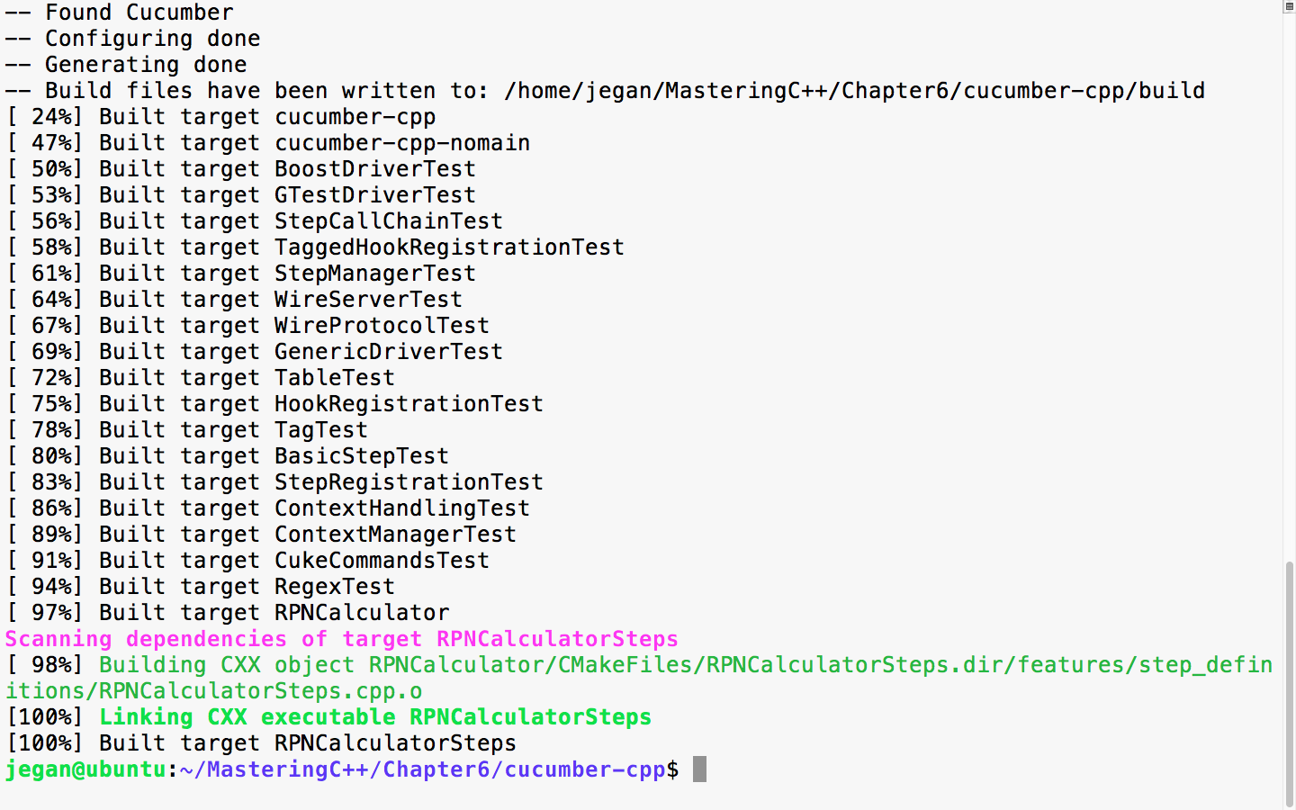
Cool! Since the code compiles without errors, let's execute the test case now and observe what happens:
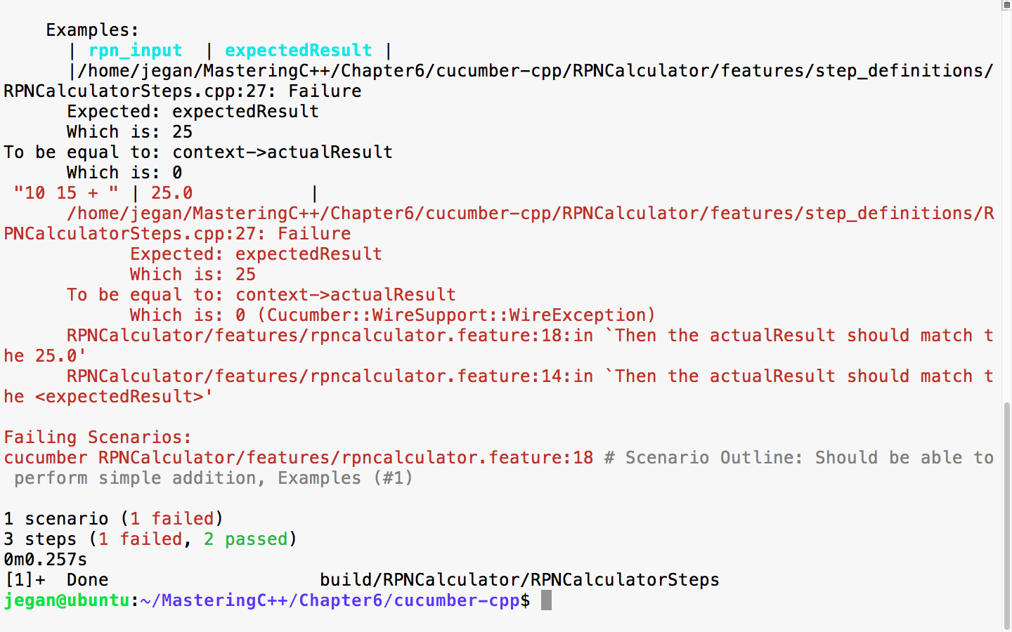
The errors are highlighted in red color as shown in the preceding screenshot by the cucumber-cpp framework. This is expected; the test case is failing as the RPNCalculator::evaluate method is hardcoded to return 0.0.
Now, let's go ahead and implement the code to make this test case pass. The modified RPNCalculator header file looks as follows:
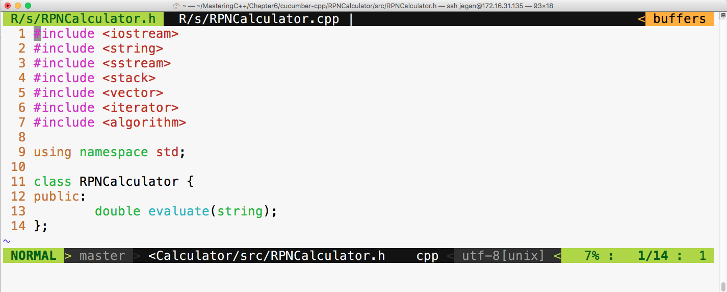
The respective RPNCalculator source file looks as follows:
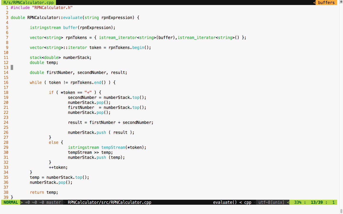
As per BDD practice, note that we have only implemented code that is necessary for supporting the addition operation alone, as per our current Cucumber scenario requirements. Like TDD, in BDD, we are supposed to write only the required amount of code to satisfy the current scenario; this way, we can ensure that every line of code is covered by effective test cases.
Let's now build and test. The following commands can be used to build, launch the steps in the background, and run the Cucumber test cases with a wire protocol, respectively:
cmake --build build

build/RPNCalculator/RPNCalculatorSteps &

cucumber RPNCalculator
The following screenshot demonstrates the procedure of building and executing the Cucumber test case:
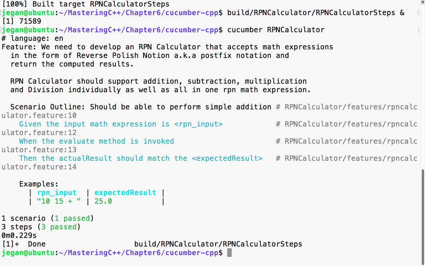
Great! Our test scenario is all green now! Let's move on to our next test scenario.
Let's add a scenario in the feature file to test the subtraction operation, as follows:
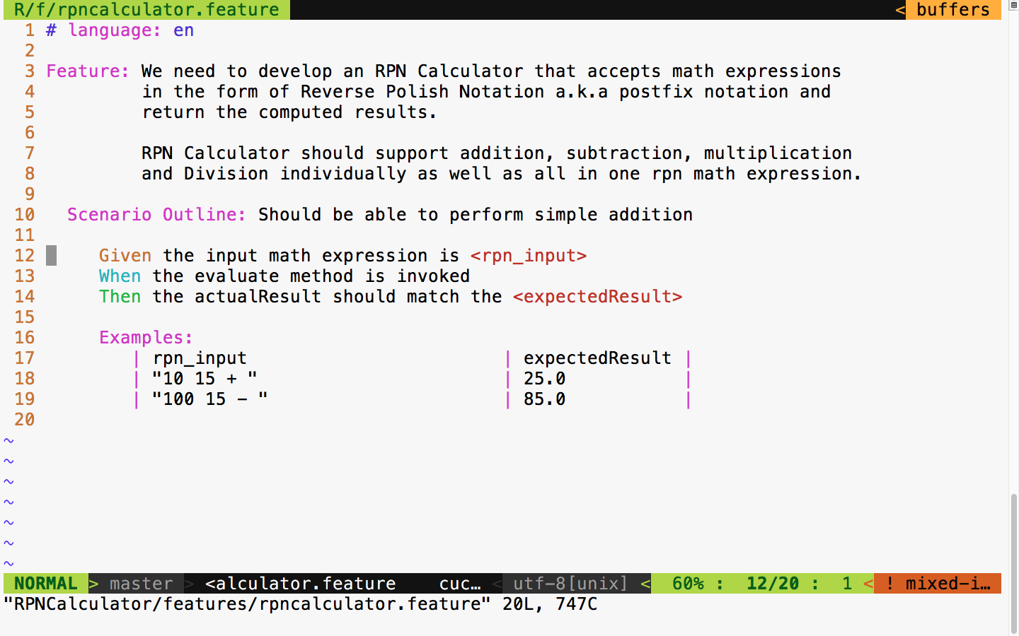
The test output looks as follows:
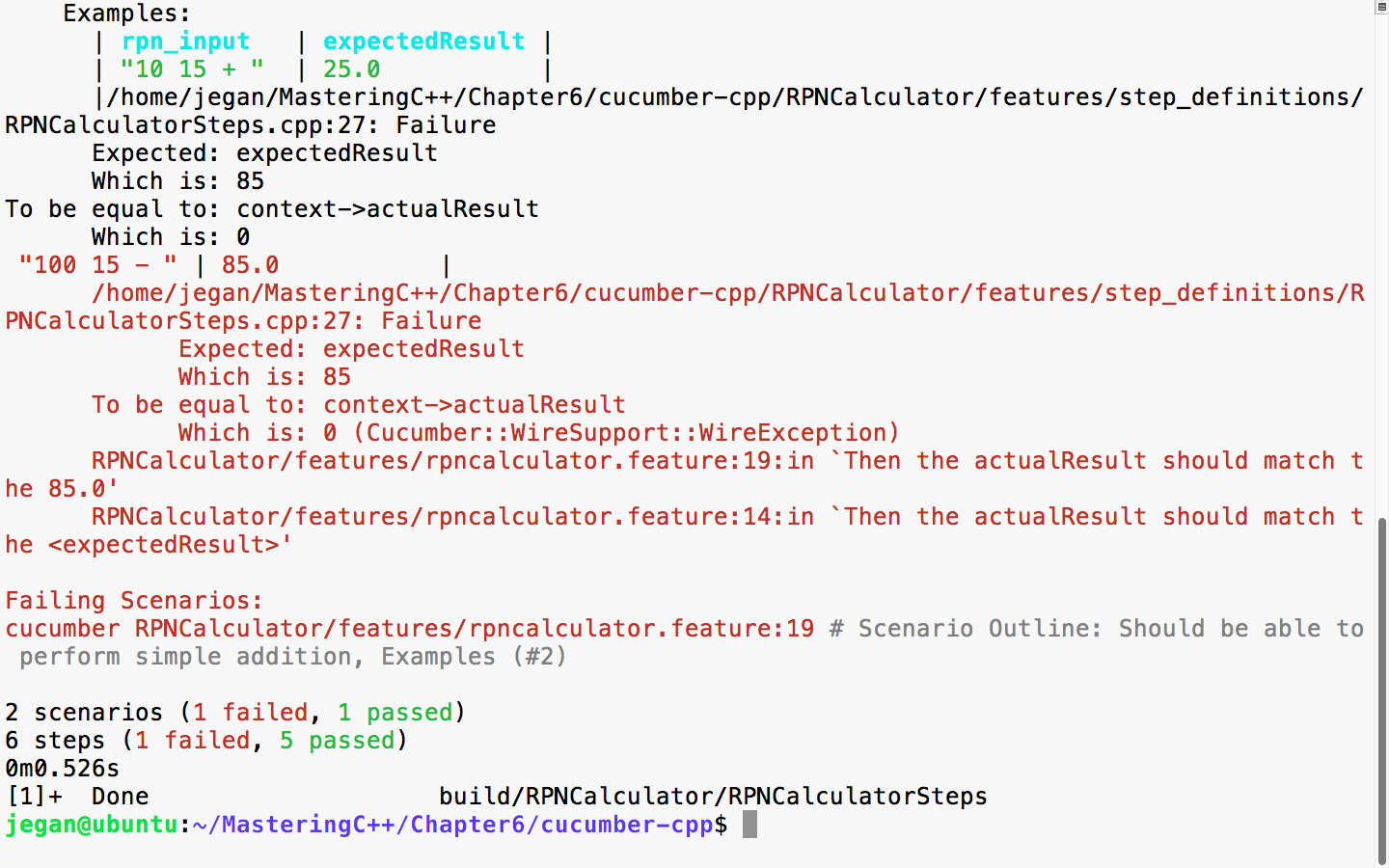
We had seen this before, hadn't we? I'm sure you guessed it right; the expected result is 85 whereas the actual result is 0, as we haven't added any support for subtraction yet. Now, let's add the necessary code to add the subtraction logic in our application:
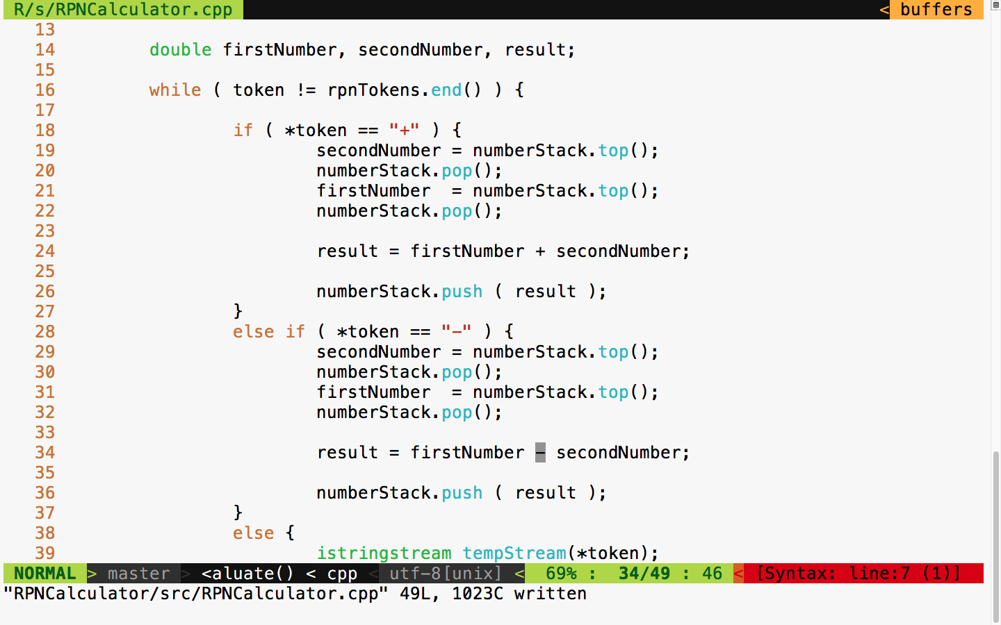
With this code change, let's rerun the test case and see what the test outcome is:
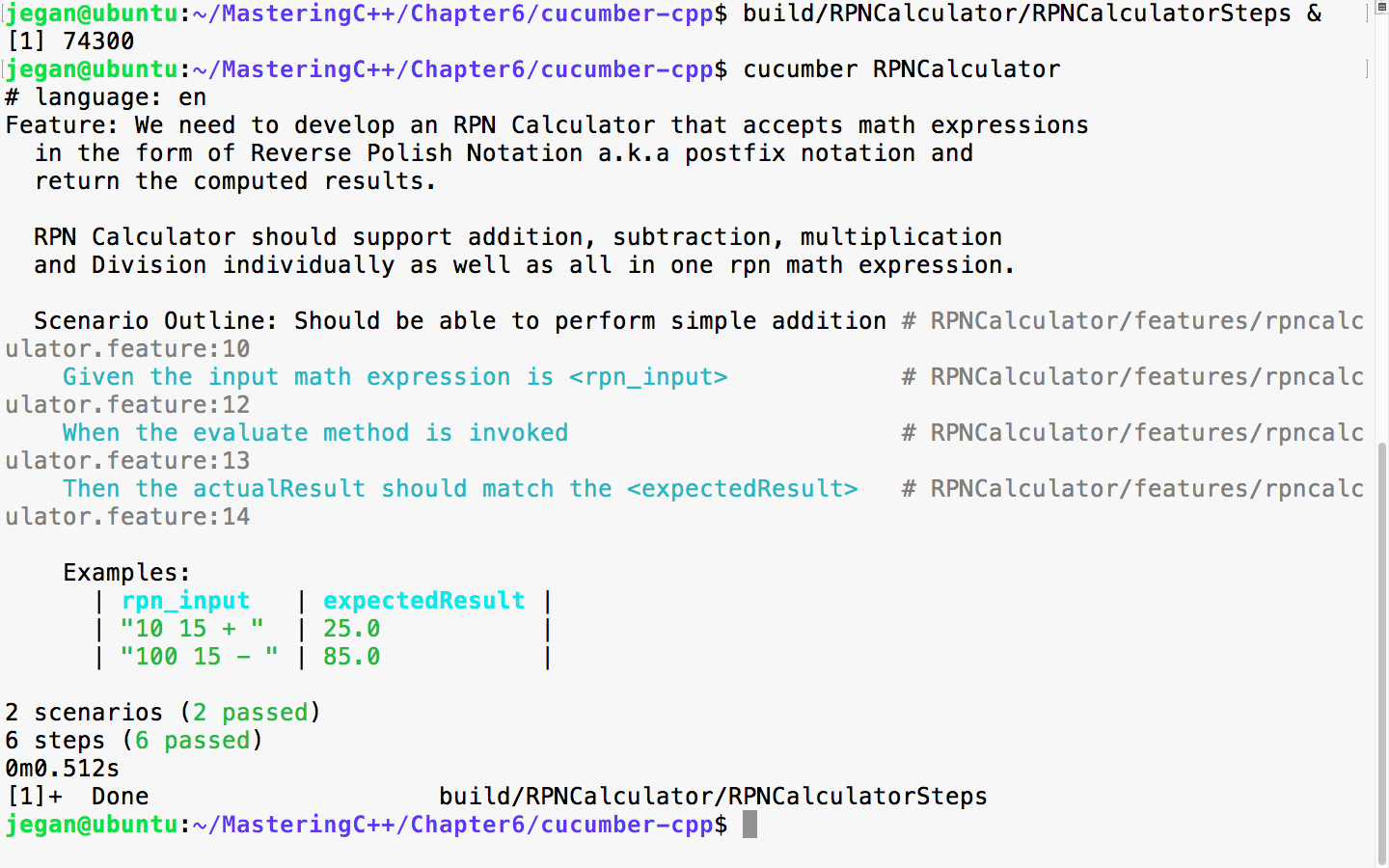
Cool, the test report is back to green!
Let's move on and add a scenario in the feature file to test the multiplication operation:
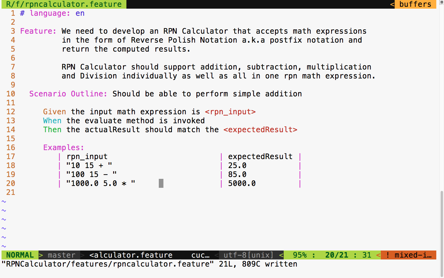
It is time to the run the test case, as shown in the following screenshot:
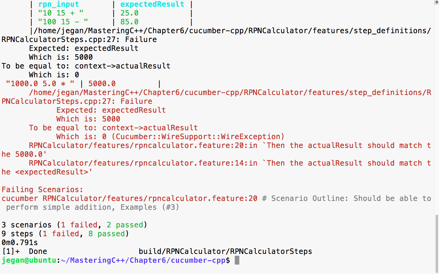
You got it right; yes, we need to add support for multiplication in our production code. Okay, let's do it right away, as shown in the following screenshot:
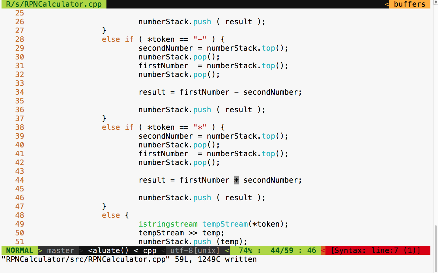
The following commands help you build, launch the steps applications, and run the Cucumber test cases, respectively. To be precise, the first command builds the test cases, while the second command launches the Cucumber steps test executable in the background mode. The third command executes the Cucumber test case that we wrote for the RPNCalculator project. The RPNCalculatorSteps executable will work as a server that Cucumber can talk to via the wire protocol. The Cucumber framework will get the connection details of the server from the cucumber.wire file kept under the step_definitions folder:
cmake --build build

build/RPNCalculator/RPNCalculatorSteps &

cucumber RPNCalculator
The following screenshot demonstrates the Cucumber test case execution procedure:
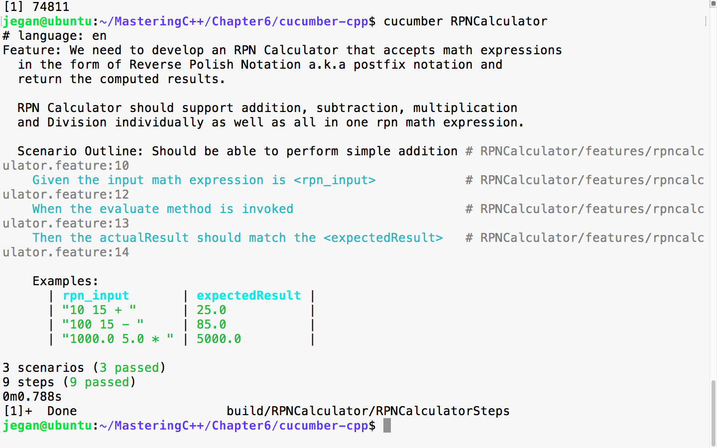
I'm sure you've got the hang of BDD! Yes, BDD is pretty simple and straightforward. Now let's add a scenario for the division operation as shown in the following screenshot:
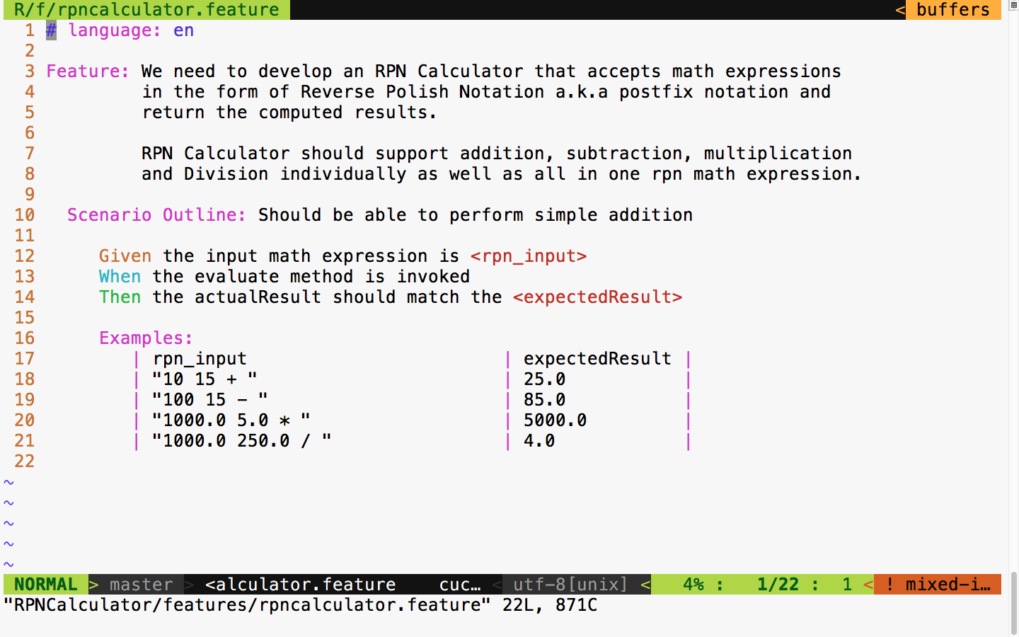
Let's quickly run the test case and observe the test outcome, as shown in the following screenshot:
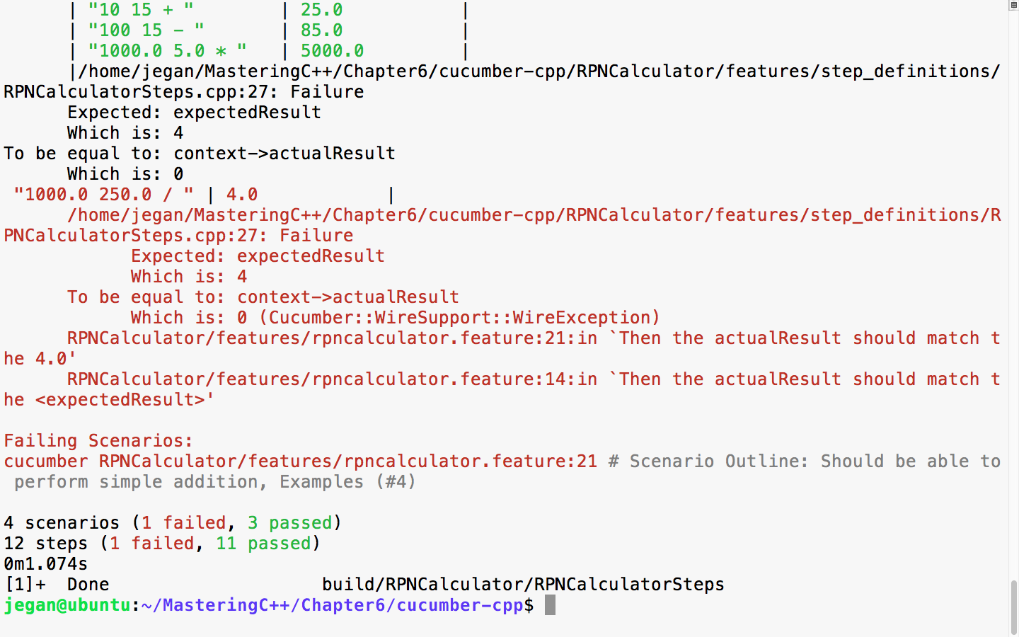
Yes, I heard you saying you know the reason for the failure. Let's quickly add support for division and rerun the test cases to see it turn all green! BDD makes coding really fun.
We need to add the following code snippet in RPNCalculator.cpp:
else if ( *token == "/" ) {
      secondNumber = numberStack.top();
      numberStack.pop();
      firstNumber = numberStack.top();
      numberStack.pop();

      result = firstNumber / secondNumber;

      numberStack.push ( result );
}
With this code change, let's check the test output:
cmake --build build
build/RPNCalculator/RPNCalculatorSteps &
cucumber RPNCalculator
The following screenshot demonstrates the procedure visually:
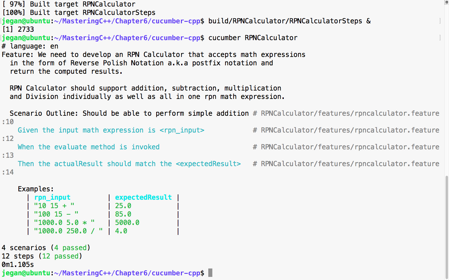
So far so good. All the scenarios we tested so far have passed, which is a good sign. But let's try a complex expression that involves many math operations. For instance, let's try 10.0 5.0 * 1.0 + 100.0 2.0 / -.
The following screenshot demonstrates the integration of the complex expression test case:
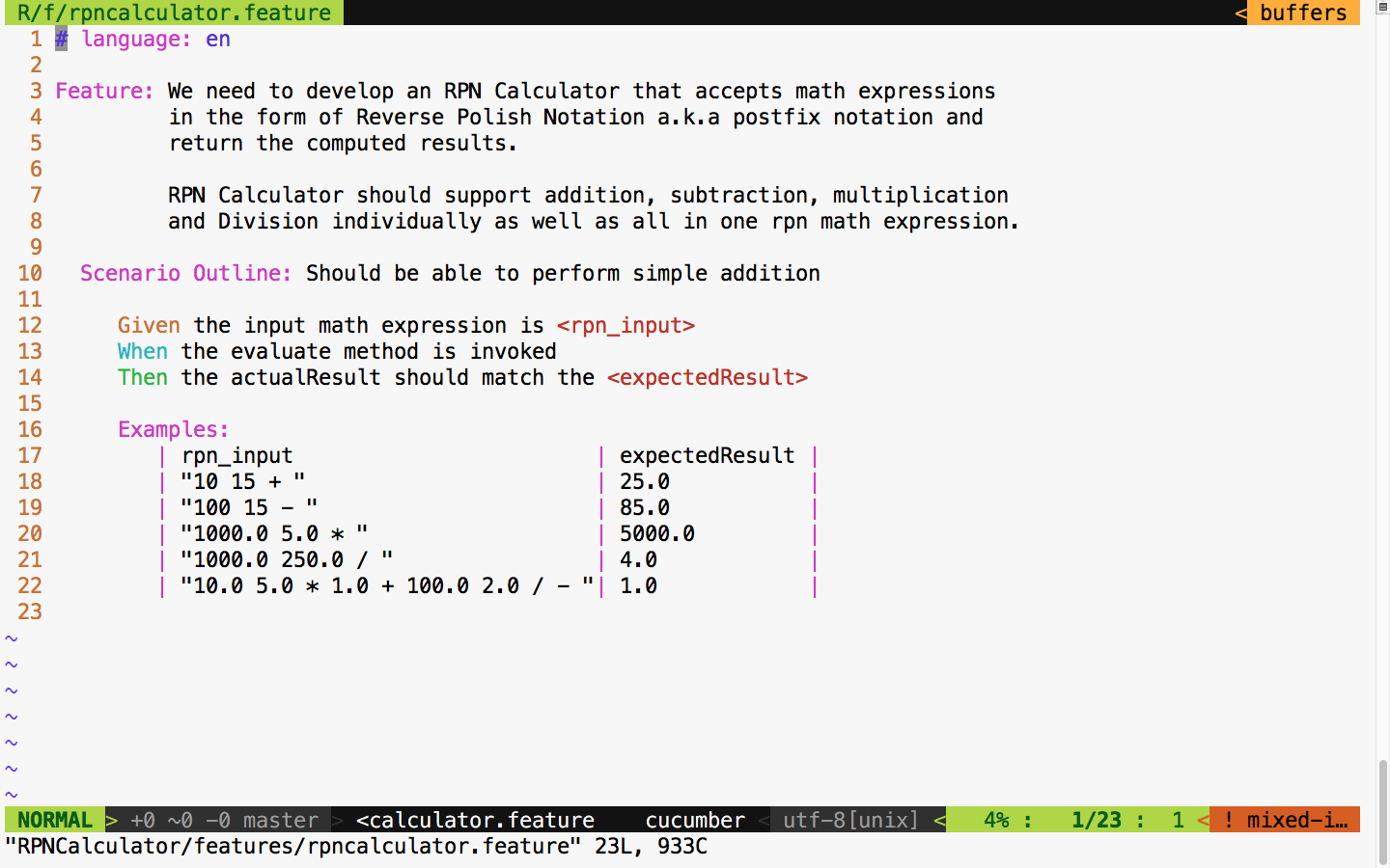
Let's run the test scenarios one more time, as this would be a real test for the entire code implemented so far, as this expression involves all the operations our simple application supports.
The following command can be used to launch the application in the background mode and to execute the Cucumber test cases:
build/RPNCalculator/RPNCalculatorSteps &
cucumber RPNCalculator
The following screenshot demonstrates the procedure visually:
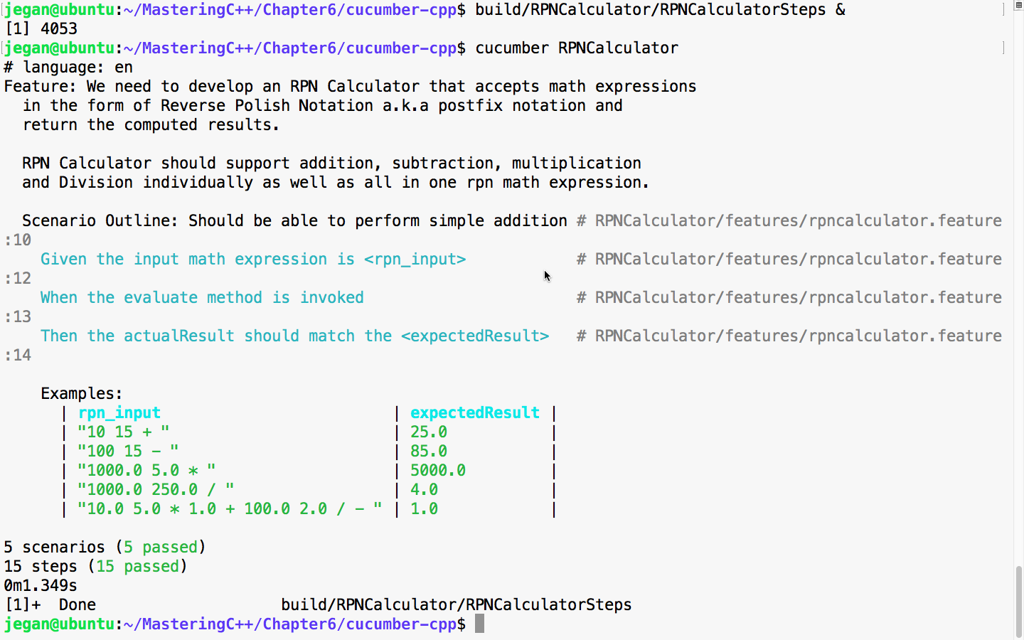
Great! If you have come this far, I'm sure you would have understood cucumber-cpp and the BDD style of coding.
In this chapter, you learned the following
In the next chapter, you will be learning about C++ debugging techniques.
This chapter will cover the following topics:
Clean code is the source code that works in an accurate way functionally and is structurally well written. Through thorough testing, we can ensure the code is functionally correct. We can improve code quality via code self-review, peer code review, code analysis, and most importantly, by code refactoring.
The following are some of the qualities of clean code:
Lastly, the best part about writing clean code is that both the development team involved in the project or product and the customer will be happy.
Refactoring helps improve the structural quality of the source code. It doesn't modify the functionality of the code; it just improves the structural aspect of the code quality. Refactoring makes the code cleaner, but at times it may help you improve the overall code performance. However, you need to understand that performance tuning is different from code refactoring.
The following diagram demonstrates the development process overview:
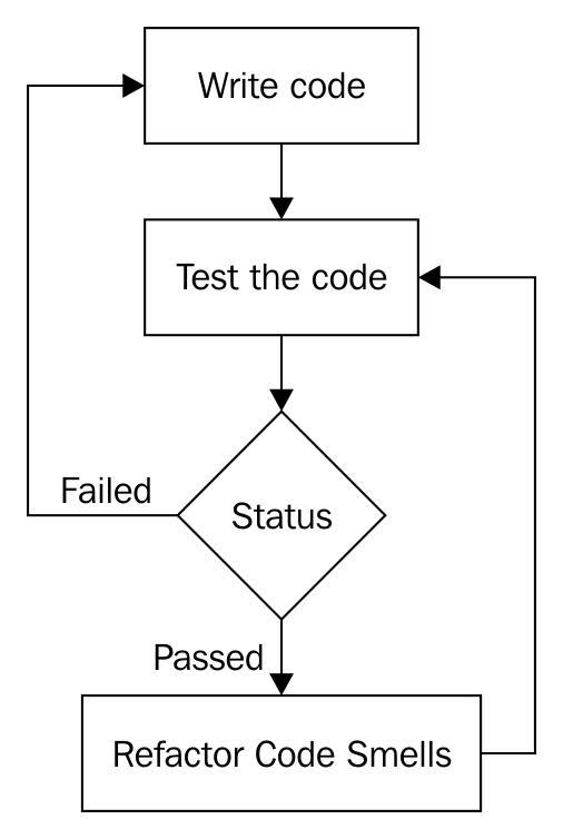
How is code refactoring done safely? The answer to this question is as follows:
Source code has two aspects of quality, namely functional and structural. The functional quality of a piece of source code can be achieved by testing the code against the customer specifications. The biggest mistake most developers make is that they tend to commit the code to version control software without refactoring it; that is, they commit the code the moment they believe it is functionally complete.
As a matter of fact, committing code to version control often is a good habit, as this is what makes continuous integration and DevOps possible. After committing the code to version control, what the vast majority of developers ignore is refactoring it. It is highly critical that you refactor the code to ensure it is clean, without which being agile is impossible.
Code that looks like noodles (spaghetti) requires more efforts to enhance or maintain. Hence, responding to a customer's request quickly is not practically possible. This is why maintaining clean code is critical to being agile. This is applicable irrespective of the agile framework that is followed in your organization.
Agile is all about fail fast. An agile team will be able to respond to a customer's requirement quickly without involving any circus from the development team. It doesn't really matter much which agile framework the team is using: Scrum, Kanban, XP, or something else. What really matters is, are you following them seriously?
As an independent software consultant, I have personally observed and learned who generally complains, and why they complain about agile.
As Scrum is one of the most popular agile frameworks, let's assume a product company, say, ABC Tech Private Ltd., has decided to follow Scrum for the new product that they are planning to develop. The good news is that ABC Tech, just like most organizations, also hosts a Sprint planning meeting, a daily stand-up meeting, Sprint review, Sprint retrospective, and all other Scrum ceremonies efficiently. Assume that ABC Tech has ensured their Scrum master is Scrum-certified and the product manager is a Scrum-certified product owner. Great! Everything sounds good so far.
Let's say the ABC Tech product team doesn't use TDD, BDD, ATDD, and DevOps. Do you think the ABC Tech product team is agile? Certainly not. As a matter of fact, the development team will be highly stressed with a hectic and impractical schedule. At the end of the day, there will be very high attrition, as the team will not be happy. Hence, customers will not be happy, as the quality of the product will suffer terribly.
What do you think has gone wrong with the ABC Tech product team?
Scrum has two sets of processes, namely the project management process, which is covered by Scrum ceremonies. Then, there is the engineering side of the process, which most organizations don't pay much attention to. This is evident from the interest or awareness of Certified SCRUM Developer (CSD) certification in the IT industry. The amount of interest the IT industry shows to CSM, CSPO, or CSP is hardly shown to CSD, which is required for developers. However, I don't believe certification alone could make someone a subject-matter expert; it only shows the seriousness the person or the organization shows in embracing an agile framework and delivering quality products to their customers.
Unless the code is kept clean, how is it possible for the development team to respond to customers' requirements quickly? In other words, unless the engineers in the development team embrace TDD, BDD, ATDD, continuous integration, and DevOps in the product development, no team will be able to succeed in Scrum or, for that matter, with any other agile framework.
The bottom line is that unless your organization takes the engineering Scrum process and project management Scrum process equally serious, no development team can claim to succeed in agile.
SOLID is an acronym for a set of important design principles that, if followed, can avoid code smells and improve the code quality, both structurally and functionally.
Code smells can be prevented or refactored into clean code if your software architecture meets the SOLID design principle compliance. The following principles are collectively called SOLID design principles:
The best part is that most design patterns also follow and are compliant with SOLID design principles.
Let's go through each of the preceding design principles one by one in the following sections.
Single responsibility principle is also referred to as SRP in short. SRP says that every class must have only one responsibility. In other words, every class must represent exactly one object. When a class represents multiple objects, it tends to violate SRP and opens up chances for multiple code smells.
For example, let's take a simple Employee class, as follows:
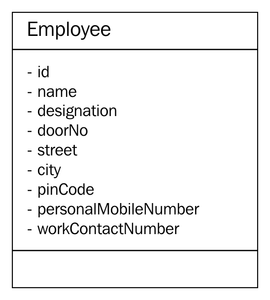
In the preceding class diagram, the Employee class seems to represent three different objects: Employee, Address, and Contact. Hence, it violates the SRP. As per this principle, from the preceding Employee class, two other classes can be extracted, namely Address and Contact, as follows:
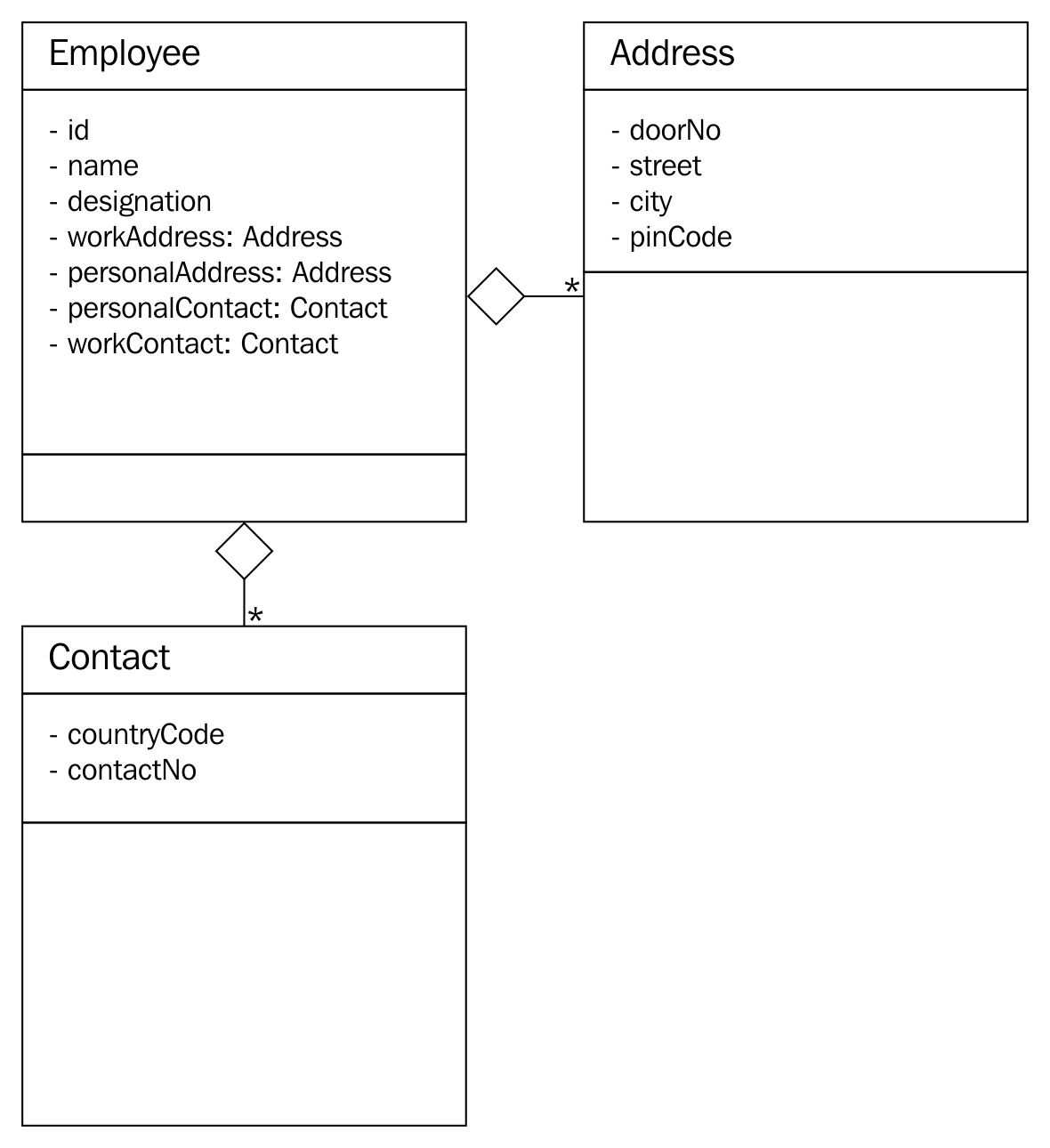
For simplicity, the class diagrams used in this section don't show any methods that are supported by the respective classes, as our focus is understanding the SRP with a simple example.
In the preceding refactored design, Employee has one or more addresses (personal and official) and one or more contacts (personal and official). The best part is that after refactoring the design, every class abstracts one and only thing; that is, it has only one responsibility.
An architecture or design is in compliance with the open closed principle (OCP) when the design supports the addition of new features with no code changes or without modifying the existing source code. As you know, based on your professional industry experience, every single project you have come across was extensible in one way or another. This is how you were able to add new features to your product. However, the design will be in compliance with the OCP when such a feature extension is done without you modifying the existing code.
Let's take a simple Item class, as shown in the following code. For simplicity, only the essential details are captured in the Item class:
#include <iostream>
#include <string>
using namespace std;
class Item {
       private:
         string name;
         double quantity;
         double pricePerUnit;
       public:
         Item ( string name, double pricePerUnit, double quantity ) {
         this-name = name;
         this->pricePerUnit = pricePerUnit;
         this->quantity = quantity;
    }
    public double getPrice( ) {
           return quantity * pricePerUnit;
    }
    public String getDescription( ) {
           return name;
    }
};
Assume the preceding Item class is part of a simple billing application for a small shop. As the Item class will be able to represent a pen, calculator, chocolate, notebook, and so on, it is generic enough to support any billable item that is dealt by the shop. However, if the shop owner is supposed to collect Goods and Services Tax (GST) or Value Added Tax (VAT), the existing Item class doesn't seem to support the tax component. One common approach is to modify the Item class to support the tax component. However, if we were to modify existing code, our design would be non-compliant to OCP.
Hence, let's refactor our design to make it OCP-compliant using Visitor design pattern. Let's explore the refactoring possibility, as shown in the following code:
#ifndef __VISITABLE_H
#define __VISITABLE_H
#include <string>
 using namespace std;
class Visitor;

class Visitable {
 public:
        virtual void accept ( Visitor * ) = 0;
        virtual double getPrice() = 0;
        virtual string getDescription() = 0;
 };
#endif
The Visitable class is an abstract class with three pure virtual functions. The Item class will be inheriting the Visitable abstract class, as shown here:
#ifndef __ITEM_H
#define __ITEM_H
#include <iostream>
#include <string>
using namespace std;
#include "Visitable.h"
#include "Visitor.h"
class Item : public Visitable {
 private:
       string name;
       double quantity;
       double unitPrice;
 public:
       Item ( string name, double quantity, double unitPrice );
       string getDescription();
       double getQuantity();
       double getPrice();
       void accept ( Visitor *pVisitor );
 };

 #endif
Next, let's take a look at the Visitor class, shown in the following code. It says there can be any number of Visitor subclasses that can be implemented in future to add new functionalities, all without modifying the Item class:
class Visitable;
#ifndef __VISITOR_H
#define __VISITOR_H
class Visitor {
 protected:
 double price;

 public:
 virtual void visit ( Visitable * ) = 0;
 virtual double getPrice() = 0;
 };

 #endif
The GSTVisitor class is the one that lets us add the GST functionality without modifying the Item class. The GSTVisitor implementation looks like this:
#include "GSTVisitor.h"

void GSTVisitor::visit ( Visitable *pItem ) {
     price = pItem->getPrice() + (0.18 * pItem->getPrice());
}

double GSTVisitor::getPrice() {
     return price;
}
The Makefile looks as follows:
all: GSTVisitor.o Item.o main.o
     g++ -o gst.exe GSTVisitor.o Item.o main.o

GSTVisitor.o: GSTVisitor.cpp Visitable.h Visitor.h
     g++ -c GSTVisitor.cpp

Item.o: Item.cpp
     g++ -c Item.cpp

main.o: main.cpp
     g++ -c main.cpp
The refactored design is OCP-compliant, as we would be able to add new functionalities without modifying the Item class. Just imagine: if the GST calculation varies from time to time, without modifying the Item class, we would be able to add new subclasses of Visitor and address the upcoming changes.
Liskov substitution principle (LSP) stresses the importance of subclasses adhering to the contract established by the base class. In an ideal inheritance hierarchy, as the design focus moves up the class hierarchy, we should notice generalization; as the design focus moves down the class hierarchy, we should notice specialization.
The inheritance contract is between two classes, hence it is the responsibility of the base class to impose rules that all subclasses can follow, and the subclasses are equally responsible for obeying the contract once agreed. A design that compromises these design philosophies will be non-compliant to the LSP.
LSP says if a method takes the base class or interface as an argument, one should be able to substitute the instance of any one of the subclasses unconditionally.
As a matter of fact, inheritance violates the most fundamental design principles: inheritance is weakly cohesive and strongly coupled. Hence, the real benefit of inheritance is polymorphism, and code reuse is a tiny benefit compared to the price paid for inheritance. When LSP is violated, we can't substitute the base class instance with one of its subclass instances, and the worst part is we can't invoke methods polymorphically. In spite of paying the design penalties of using inheritance, if we can't reap the benefit of polymorphism, there is no real motivation to use it.
The technique to identify LSP violation is as follows:
The following are the ways to refactor LSP violations:
Interface segregation design principle recommends modeling many small interfaces for a specific purpose, as opposed to modeling one bigger interface that represents many things. In the case of C++, an abstract class with pure virtual functions can be thought of as an interface.
Let's take a simple example to understand interface segregation:
#include <iostream>
#include <string>
using namespace std;

class IEmployee {
      public:
          virtual string getDoor() = 0;
          virtual string getStreet() = 0;
          virtual string getCity() = 0;
          virtual string getPinCode() = 0;
          virtual string getState() = 0;
          virtual string getCountry() = 0;
          virtual string getName() = 0;
          virtual string getTitle() = 0;
          virtual string getCountryDialCode() = 0;
          virtual string getContactNumber() = 0;
};
In the preceding example, the abstract class demonstrates a chaotic design. The design is chaotic as it seems to represent many things, such as employee, address, and contact. One of the ways in which the preceding abstract class can be refactored is by breaking the single interface into three separate interfaces: IEmployee, IAddress, and IContact. In C++, interfaces are nothing but abstract classes with pure virtual functions:
#include <iostream>
#include <string>
#include <list>
using namespace std;

class IEmployee {
  private:
     string firstName, middleName, lastName,
     string title;
     string employeeCode;
     list<IAddress> addresses;
     list<IContact> contactNumbers;
  public:
     virtual string getAddress() = 0;
     virtual string getContactNumber() = 0;
};

class IAddress {
     private:
          string doorNo, street, city, pinCode, state, country;
     public:
          IAddress ( string doorNo, string street, string city,
            string pinCode, string state, string country );
          virtual string getAddress() = 0;
};

class IContact {
      private:
           string countryCode, mobileNumber;
      public:
           IContact ( string countryCode, string mobileNumber );
           virtual string getMobileNumber() = 0;
};
In the refactored code snippet, every interface represents exactly one object, hence it is in compliance with the interface segregation design principle.
A good design will be strongly cohesive and loosely coupled. Hence, our design must have less dependency. A design that makes a code dependent on many other objects or modules is considered a poor design. If Dependency Inversion (DI) is violated, any change that happens in the dependent modules will have a bad impact on our module, leading to a ripple effect.
Let's take a simple example to understand the power of DI. A Mobile class "has a" Camera object and notice that has a form is composition. Composition is an exclusive ownership where the lifetime of the Camera object is directly controlled by the Mobile object:

As you can see in the preceding image, the Mobile class has an instance of Camera and the has a form used is composition, which is an exclusive ownership relationship.
Let's take a look at the Mobile class implementation, as follows:
#include <iostream>
using namespace std;

class Mobile {
     private:
          Camera camera;
     public:
          Mobile ( );
          bool powerOn();
          bool powerOff();
};

class Camera {
      public:
          bool ON();
          bool OFF();
};

bool Mobile::powerOn() {
       if ( camera.ON() ) {
           cout << "nPositive Logic - assume some complex Mobile power ON logic happens here." << endl;
           return true;
       }
       cout << "nNegative Logic - assume some complex Mobile power OFF logic happens here." << endl;
            << endl;
       return false;
}

bool Mobile::powerOff() {
      if ( camera.OFF() ) {
              cout << "nPositive Logic - assume some complex Mobile power OFF             logic happens here." << endl;
      return true;
 }
      cout << "nNegative Logic - assume some complex Mobile power OFF logic happens here." << endl;
      return false;
}

bool Camera::ON() {
     cout << "nAssume Camera class interacts with Camera hardware heren" << endl;
     cout << "nAssume some Camera ON logic happens here" << endl;
     return true;
}

bool Camera::OFF() {
 cout << "nAssume Camera class interacts with Camera hardware heren" << endl;
 cout << "nAssume some Camera OFF logic happens here" << endl;
 return true;
}
In the preceding code, Mobile has implementation-level knowledge about Camera, which is a poor design. Ideally, Mobile should be interacting with Camera via an interface or an abstract class with pure virtual functions, as this separates the Camera implementation from its contract. This approach helps replace Camera without affecting Mobile and also gives an opportunity to support a bunch of Camera subclasses in place of one single camera.
Wondering why it is called Dependency Injection (DI) or Inversion of Control (IOC)? The reason it is termed dependency injection is that currently, the lifetime of Camera is controlled by the Mobile object; that is, Camera is instantiated and destroyed by the Mobile object. In such a case, it is almost impossible to unit test Mobile in the absence of Camera, as Mobile has a hard dependency on Camera. Unless Camera is implemented, we can't test the functionality of Mobile, which is a bad design approach. When we invert the dependency, it lets the Mobile object use the Camera object while it gives up the responsibility of controlling the lifetime of the Camera object. This process is rightly referred to as IOC. The advantage is that you will be able to unit test the Mobile and Camera objects independently and they will be strongly cohesive and loosely coupled due to IOC.
Let's refactor the preceding code with the DI design principle:
#include <iostream>
using namespace std;

class ICamera {
       public:
         virtual bool ON() = 0;
         virtual bool OFF() = 0;
};

class Mobile {
      private:
            ICamera *pCamera;
      public:
            Mobile ( ICamera *pCamera );
            void setCamera( ICamera *pCamera );
            bool powerOn();
            bool powerOff();
};

class Camera : public ICamera {
public:
            bool ON();
            bool OFF();
};

//Constructor Dependency Injection
Mobile::Mobile ( ICamera *pCamera ) {
    this->pCamera = pCamera;
}

//Method Dependency Injection
Mobile::setCamera( ICamera *pCamera ) {
    this->pCamera = pCamera;
}

bool Mobile::powerOn() {
      if ( pCamera->ON() ) {
            cout << "nPositive Logic - assume some complex Mobile power ON logic happens here." << endl;
            return true;
      }
cout << "nNegative Logic - assume some complex Mobile power OFF logic happens here." << endl;
<< endl;
      return false;
}

bool Mobile::powerOff() {
      if ( pCamera->OFF() ) {
           cout << "nPositive Logic - assume some complex Mobile power OFF logic happens here." << endl;
           return true;
}
      cout << "nNegative Logic - assume some complex Mobile power OFF logic happens here." << endl;
      return false;
}

bool Camera::ON() {
       cout << "nAssume Camera class interacts with Camera hardware heren" << endl;
       cout << "nAssume some Camera ON logic happens here" << endl;
       return true;
}

bool Camera::OFF() {
       cout << "nAssume Camera class interacts with Camera hardware heren" << endl;
       cout << "nAssume some Camera OFF logic happens here" << endl;
       return true;
}
The changes are highlighted in bold in the preceding code snippet. IOC is such a powerful technique that it lets us decouple the dependency as just demonstrated; however, its implementation is quite simple.
Code smell is a term used to refer to a piece of code that lacks structural quality; however, the code may be functionally correct. Code smells violate SOLID design principles, hence they must be taken seriously, as the code that is not well written leads to heavy maintenance cost in the long run. However, code smells can be refactored into clean code.
As an independent software consultant, I have had a lot of opportunities to interact and learn from great developers, architects, QA folks, system administrators, CTOs and CEOs, entrepreneurs, and so on. Whenever our discussions crossed the billion dollar question, "What is clean code or good code?", I more or less got one common response globally, "Good code will be well commented." While this is partially correct, certainly that's where the problem starts. Ideally, clean code should be self-explanatory, without any need for comments. However, there are some occasions where comments improve the overall readability and maintainability. Not all comments are code smells, hence it becomes necessary to differentiate a good comment from a bad one. Have a look at the following code snippet:
if ( condition1 ) {
     // some block of code
}
else if ( condition2 ) {
     // some block of code
}
else {
     // OOPS - the control should not reach here ### Code Smell ###
}
I'm sure you have come across these kinds of comments. Needless to explain that the preceding scenario is a code smell. Ideally, the developer should have refactored the code to fix the bug instead of writing such a comment. I was once debugging a critical issue in the middle of the night and I noticed the control reached the mysterious empty code block with just a comment in it. I'm sure you have come across funnier code and can imagine the frustration it brings; at times, you too would have written such a type of code.
A good comment will express why the code is written in a specific way rather than express how the code does something. A comment that conveys how the code does something is a code smell, whereas a comment that conveys the why part of the code is a good comment, as the why part is not expressed by the code; therefore, a good comment provides value addition.
A method is long when it is identified to have multiple responsibilities. Naturally, a method that has more than 20-25 lines of code tends to have more than one responsibility. Having said that, a method with more lines of code is longer. This doesn't mean a method with less than 25 lines of code isn't longer. Take a look at the following code snippet:
void Employee::validateAndSave( ) {
        if ( ( street != "" ) && ( city != "" ) )
              saveEmployeeDetails();
}
Clearly, the preceding method has multiple responsibilities; that is, it seems to validate and save the details. While validating before saving isn't wrong, the same method shouldn't do both. So the preceding method can be refactored into two smaller methods that have one single responsibility:
private:
void Employee::validateAddress( ) {
     if ( ( street == "" ) || ( city == "" ) )
          throw exception("Invalid Address");
}

public:
void Employee::save() {
      validateAddress();
}
Each of the refactored methods shown in the preceding code has exactly one responsibility. It would be tempting to make the validateAddress() method a predicate method; that is, a method that returns a bool. However, if validateAddress() is written as a predicate method, then the client code will be forced to do if check, which is a code smell. Handling errors by returning error code isn't considered object-oriented code, hence error handling must be done using C++ exceptions.
An object-oriented method takes fewer arguments, as a well-designed object will be strongly cohesive and loosely coupled. A method that takes too many arguments is a symptom that informs that the knowledge required to make a decision is received externally, which means the current object doesn't have all of the knowledge to make a decision by itself.
This means the current object is weakly cohesive and strongly coupled, as it depends on too much external data to make a decision. Member functions generally tend to receive fewer arguments, as the data members they require are generally member variables. Hence, the need to pass member variables to member functions sounds artificial.
Let's see some of the common reasons why a method tends to receive too many arguments. The most common symptoms and reasons are listed here:
The ways to refactor a method that takes long parameter list (LPL) are listed here:
Duplicate code is a commonly recurring code smell that doesn't require much explanation. The copying and pasting code culture alone can't be blamed for duplicate code. Duplicate code makes code maintenance more cumbersome, as the same issues may have to be fixed in multiple places, and integrating new features requires too many code changes, which tends to break the unexpected functionalities. Duplicate code also increases the application binary footprint, hence it must be refactored to clean code.
Conditional complexity code smell is about complex large conditions that tend to grow larger and more complex with time. This code smell can be refactored with the strategy design pattern. As the strategy design pattern deals with many related objects, there is scope for using the Factory method, and the null object design pattern can be used to deal with unsupported subclasses in the Factory method:
//Before refactoring
void SomeClass::someMethod( ) {
      if (  ! conition1 && condition2 )
         //perform some logic
      else if ( ! condition3 && condition4 && condition5 )
         //perform some logic
      else
         //do something
}

//After refactoring
void SomeClass::someMethod() {
     if ( privateMethod1() )
          //perform some logic
     else if ( privateMethod2() )
          //perform some logic
     else
         //do something
}
A large class code smell makes the code difficult to understand and tougher to maintain. A large class can do too many things for one class. Large classes can be refactored by breaking them into smaller classes with a single responsibility.
Dead code is commented code or code that is never used or integrated. It can be detected with code coverage tools. Generally, developers retain these instances of code due to lack of confidence, and this happens more often in legacy code. As every code is tracked in version control software tools, dead code can be deleted, and if required, can always be retrieved back from version control software.
Primitive Obsession (PO) is a wrong design choice: use of a primitive data type to represent a complex domain entity. For example, if the string data type is used to represent date, though it sounds like a smart idea initially, it invites a lot of maintenance trouble in the long run.
Assuming you have used a string data type to represent date, the following issues will be a challenge:
Ideally, date must be represented by a class as opposed to a primitive data type.
Data classes provide only getter and setter functions. Though they are very good for transferring data from one layer to another, they tend to burden the classes that depend on the data class. As data classes won't provide any useful functionalities, the classes that interact or depend on data classes end up adding functionalities with the data from the data class. In this fashion, the classes around the data class violate the SRP and tend to be a large class.
Certain classes are termed feature envy if they have too much knowledge about other internal details of other classes. Generally, this happens when the other classes are data classes. Code smells are interrelated; breaking one code smell tends to attract other code smells.
In this chapter, you learned about the following topics:
You also learned about many refactoring techniques that will help you maintain your code cleaner. Happy coding!
Chances are that if you're reading this book, you have already done some multithreaded programming in C++, or, possibly, other languages. This chapter is meant to recap the topic purely from a C++ point of view, going through a basic multithreaded application, while also covering the tools we'll be using throughout the book. At the end of this chapter, you will have all the knowledge and information needed to proceed with the further chapters.
Topics covered in this chapter include the following:
During the course of this book, we'll be assuming the use of a GCC-based toolchain (GCC or MinGW on Windows). If you wish to use alternative toolchains (clang, MSVC, ICC, and so on), please consult the documentation provided with these for compatible commands.
To compile the examples provided in this book, makefiles will be used. For those unfamiliar with makefiles, they are a simple but powerful text-based format used with the make tool for automating build tasks including compiling source code and adjusting the build environment. First released in 1977, make remains among the most popular build automation tools today.
Familiarity with the command line (Bash or equivalent) is assumed, with MSYS2 (Bash on Windows) recommended for those using Windows.
In its most basic form, a multithreaded application consists of a singular process with two or more threads. These threads can be used in a variety of ways; for example, to allow the process to respond to events in an asynchronous manner by using one thread per incoming event or type of event, or to speed up the processing of data by splitting the work across multiple threads.
Examples of asynchronous responses to events include the processing of the graphical user interface (GUI) and network events on separate threads so that neither type of event has to wait on the other, or can block events from being responded to in time. Generally, a single thread performs a single task, such as the processing of GUI or network events, or the processing of data.
For this basic example, the application will start with a singular thread, which will then launch a number of threads, and wait for them to finish. Each of these new threads will perform its own task before finishing.
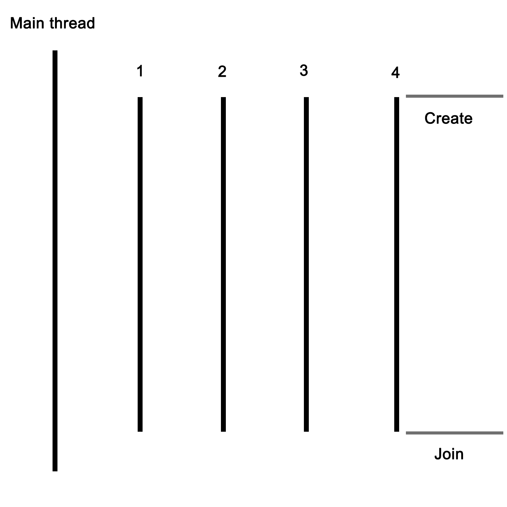
Let's start with the includes and global variables for our application:
#include <iostream>
#include <thread>
#include <mutex>
#include <vector>
#include <random>

using namespace std;

// --- Globals
mutex values_mtx;
mutex cout_mtx;
vector<int> values;
Both the I/O stream and vector headers should be familiar to anyone who has ever used C++: the former is here used for the standard output (cout), and the vector for storing a sequence of values.
The random header is new in c++11, and as the name suggests, it offers classes and methods for generating random sequences. We use it here to make our threads do something interesting.
Finally, the thread and mutex includes are the core of our multithreaded application; they provide the basic means for creating threads, and allow for thread-safe interactions between them.
Moving on, we create two mutexes: one for the global vector and one for cout, since the latter is not thread-safe.
Next we create the main function as follows:
int main() {
    values.push_back(42);
We push a fixed value onto the vector instance; this one will be used by the threads we create in a moment:
    thread tr1(threadFnc, 1);
    thread tr2(threadFnc, 2);
    thread tr3(threadFnc, 3);
    thread tr4(threadFnc, 4);
We create new threads, and provide them with the name of the method to use, passing along any parameters--in this case, just a single integer:
    tr1.join();
    tr2.join();
    tr3.join();
    tr4.join();
Next, we wait for each thread to finish before we continue by calling join() on each thread instance:
    cout << "Input: " << values[0] << ", Result 1: " << values[1] << ", Result 2: " << values[2] << ", Result 3: " << values[3] << ", Result 4: " << values[4] << "n";


    return 1;
}
At this point, we expect that each thread has done whatever it's supposed to do, and added the result to the vector, which we then read out and show the user.
Of course, this shows almost nothing of what really happens in the application, mostly just the essential simplicity of using threads. Next, let's see what happens inside this method that we pass to each thread instance:
void threadFnc(int tid) {
    cout_mtx.lock();
    cout << "Starting thread " << tid << ".n";
    cout_mtx.unlock();
In the preceding code, we can see that the integer parameter being passed to the thread method is a thread identifier. To indicate that the thread is starting, a message containing the thread identifier is output. Since we're using a non-thread-safe method for this, we use the cout_mtx mutex instance to do this safely, ensuring that just one thread can write to cout at any time:
    values_mtx.lock();
    int val = values[0];
    values_mtx.unlock();
When we obtain the initial value set in the vector, we copy it to a local variable so that we can immediately release the mutex for the vector to enable other threads to use the vector:
    int rval = randGen(0, 10);
    val += rval;
These last two lines contain the essence of what the threads created do: they take the initial value, and add a randomly generated value to it. The randGen() method takes two parameters, defining the range of the returned value:
    cout_mtx.lock();
    cout << "Thread " << tid << " adding " << rval << ". New value: " << val << ".n";
    cout_mtx.unlock();

    values_mtx.lock();
    values.push_back(val);
    values_mtx.unlock();
}
Finally, we (safely) log a message informing the user of the result of this action before adding the new value to the vector. In both cases, we use the respective mutex to ensure that there can be no overlap when accessing the resource with any of the other threads.
Once the method reaches this point, the thread containing it will terminate, and the main thread will have one less thread to wait for to rejoin. The joining of a thread basically means that it stops existing, usually with a return value passed to the thread which created the thread. This can happen explicitly, with the main thread waiting for the child thread to finish, or in the background.
Lastly, we'll take a look at the randGen() method. Here we can see some multithreaded specific additions as well:
int randGen(const int& min, const int& max) {
    static thread_local mt19937 generator(hash<thread::id>()(this_thread::get_id()));
    uniform_int_distribution<int> distribution(min, max);
    return distribution(generator)
}
This preceding method takes a minimum and maximum value as explained earlier, which limits the range of the random numbers this method can return. At its core, it uses a mt19937-based generator, which employs a 32-bit Mersenne Twister algorithm with a state size of 19937 bits. This is a common and appropriate choice for most applications.
Of note here is the use of the thread_local keyword. What this means is that even though it is defined as a static variable, its scope will be limited to the thread using it. Every thread will thus create its own generator instance, which is important when using the random number API in the STL.
A hash of the internal thread identifier is used as a seed for the generator. This ensures that each thread gets a fairly unique seed for its generator instance, allowing for better random number sequences.
Finally, we create a new uniform_int_distribution instance using the provided minimum and maximum limits, and use it together with the generator instance to generate the random number which we return.
In order to compile the code described earlier, one could use an IDE, or type the command on the command line. As mentioned in the beginning of this chapter, we'll be using makefiles for the examples in this book. The big advantages of this are that one does not have to repeatedly type in the same extensive command, and it is portable to any system which supports make.
Further advantages include being able to have previous generated artifacts removed automatically and to only compile those source files which have changed, along with a detailed control over build steps.
The makefile for this example is rather basic:
GCC := g++

OUTPUT := ch01_mt_example
SOURCES := $(wildcard *.cpp)
CCFLAGS := -std=c++11 -pthread

all: $(OUTPUT)

$(OUTPUT):
    $(GCC) -o $(OUTPUT) $(CCFLAGS) $(SOURCES)

clean:
    rm $(OUTPUT)

.PHONY: all
From the top down, we first define the compiler that we'll use (g++), set the name of the output binary (the .exe extension on Windows will be post-fixed automatically), followed by the gathering of the sources and any important compiler flags.
The wildcard feature allows one to collect the names of all files matching the string following it in one go without having to define the name of each source file in the folder individually.
For the compiler flags, we're only really interested in enabling the c++11 features, for which GCC still requires one to supply this compiler flag.
For the all method, we just tell make to run g++ with the supplied information. Next we define a simple clean method which just removes the produced binary, and finally, we tell make to not interpret any folder or file named all in the folder, but to use the internal method with the .PHONY section.
When we run this makefile, we see the following command-line output:
$ make
g++ -o ch01_mt_example -std=c++11 ch01_mt_example.cpp
Afterwards, we find an executable file called ch01_mt_example (with the .exe extension attached on Windows) in the same folder. Executing this binary will result in a command-line output akin to the following:
$ ./ch01_mt_example.exe

Starting thread 1.

Thread 1 adding 8. New value: 50.

Starting thread 2.

Thread 2 adding 2. New value: 44.

Starting thread 3.

Starting thread 4.

Thread 3 adding 0. New value: 42.

Thread 4 adding 8. New value: 50.

Input: 42, Result 1: 50, Result 2: 44, Result 3: 42, Result 4: 50
What one can see here already is the somewhat asynchronous nature of threads and their output. While threads 1 and 2 appear to run synchronously, starting and quitting seemingly in order, threads 3 and 4 clearly run asynchronously as both start simultaneously before logging their action. For this reason, and especially in longer-running threads, it's virtually impossible to say in which order the log output and results will be returned.
While we use a simple vector to collect the results of the threads, there is no saying whether Result 1 truly originates from the thread which we assigned ID 1 in the beginning. If we need this information, we need to extend the data we return by using an information structure with details on the processing thread or similar.
One could, for example, use struct like this:
struct result {
    int tid;
    int result;
};
The vector would then be changed to contain result instances rather than integer instances. One could pass the initial integer value directly to the thread as part of its parameters, or pass it via some other way.
The example in this chapter is primarily useful for applications where data or tasks have to be handled in parallel. For the earlier mentioned use case of a GUI-based application with business logic and network-related features, the basic setup of a main application, which launches the required threads, would remain the same. However, instead of having each thread to be the same, each would be a completely different method.
For this type of application, the thread layout would look like this:
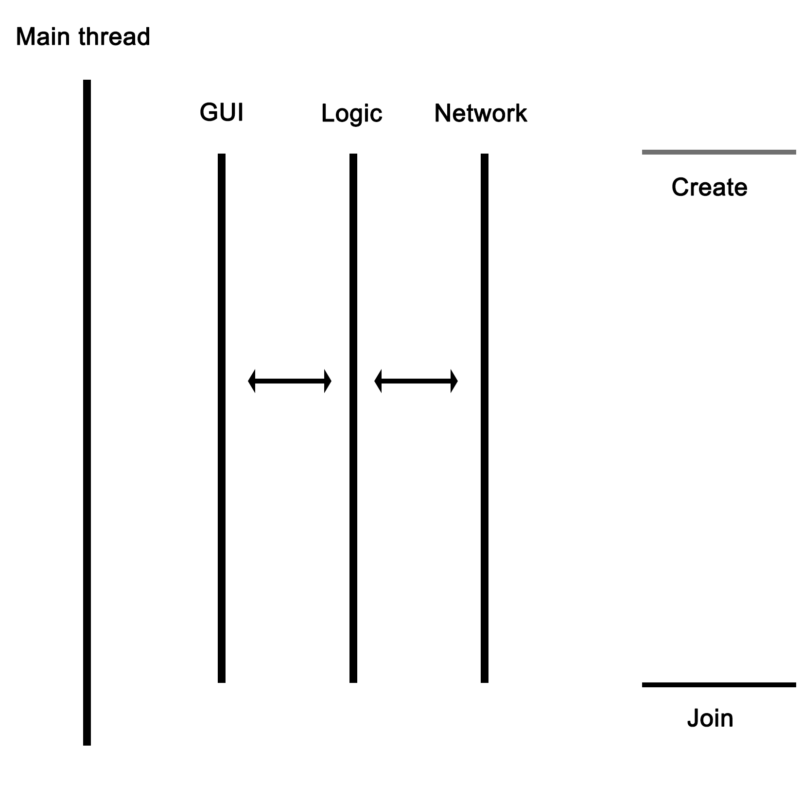
As the graphic shows, the main thread would launch the GUI, network, and business logic thread, with the latter communicating with the network thread to send and receive data. The business logic thread would also receive user input from the GUI thread, and send updates back to be displayed on the GUI.
In this chapter, we went over the basics of a multithreaded application in C++ using the native threading API. We looked at how to have multiple threads perform a task in parallel, and also explored how to properly use the random number API in the STL within a multithreaded application.
In the next chapter, we'll discuss how multithreading is implemented both in hardware and in operating systems. We'll see how this implementation differs per processor architecture and operating system, and how this affects our multithreaded application.
The foundation of any multithreaded application is formed by the implementation of the required features by the hardware of the processor, as well as by the way these features are translated into an API for use by applications by the operating system. An understanding of this foundation is crucial for developing an intuitive understanding of how to best implement a multithreaded application.
Topics covered in this chapter include the following:
Unix, Linux, and macOS are largely compliant with the POSIX standard. Portable Operating System Interface for Unix (POSIX) is an IEEE standard that helps all Unix and Unix-like operating systems, that is Linux and macOS, communicate with a single interface.
Interestingly, POSIX is also supported by POSIX-compliant tools--Cygwin, MinGW, and Windows subsystem for Linux--that provide a pseudo-Unix-like runtime and development environment on Windows platforms.
Note that pthread is a POSIX-compliant C library used in Unix, Linux, and macOS. Starting from C++11, C++ natively supports threads via the C++ thread support library and concurrent library. In this chapter, we will understand how to use pthreads, thread support, and concurrency library in an object-oriented fashion. Also, we will discuss the merits of using native C++ thread support and concurrency library as opposed to using POSIX pthreads or other third-party threading frameworks.
Let's get straight to business. You need to understand the pthread APIs we'll discuss to get your hands dirty. To start with, this function is used to create a new thread:
 #include <pthread.h>
 int pthread_create(
              pthread_t *thread,
              const pthread_attr_t *attr,
              void *(*start_routine)(void*),
              void *arg
 )
The following table briefly explains the arguments used in the preceding function:
|
API arguments |
Comments |
|
pthread_t *thread |
Thread handle pointer |
|
pthread_attr_t *attr |
Thread attribute |
|
void *(*start_routine)(void*) |
Thread function pointer |
|
void * arg |
Thread argument |
This function blocks the caller thread until the thread passed in the first argument exits, as shown in the code:
int pthread_join ( pthread_t *thread, void **retval )
The following table briefly describes the arguments in the preceding function:
|
API arguments |
Comments |
|
pthread_t thread |
Thread handle |
|
void **retval |
Output parameter that indicates the exit code of the thread procedure |
The ensuing function should be used within the thread context. Here, retval is the exit code of the thread that indicates the exit code of the thread that invoked this function:
int pthread_exit ( void *retval )
Here's the argument used in this function:
|
API argument |
Comment |
|
void *retval |
The exit code of the thread procedure |
The following function returns the thread ID:
pthread_t pthread_self(void)
Let's write our first multithreaded application:
#include <pthread.h>
#include <iostream>

using namespace std;

void* threadProc ( void *param ) {
  for (int count=0; count<3; ++count)
    cout << "Message " << count << " from " << pthread_self()
         << endl;
  pthread_exit(0);
}

int main() {
  pthread_t thread1, thread2, thread3;

  pthread_create ( &thread1, NULL, threadProc, NULL );
  pthread_create ( &thread2, NULL, threadProc, NULL );
  pthread_create ( &thread3, NULL, threadProc, NULL );

  pthread_join( thread1, NULL );
  pthread_join( thread2, NULL );

  pthread_join( thread3, NULL );

  return 0;

}
The program can be compiled with the following command:
g++ main.cpp -lpthread
As you can see, we need to link the POSIX pthread library dynamically.
Check out the following screenshot and visualize the output of the multithreaded program:
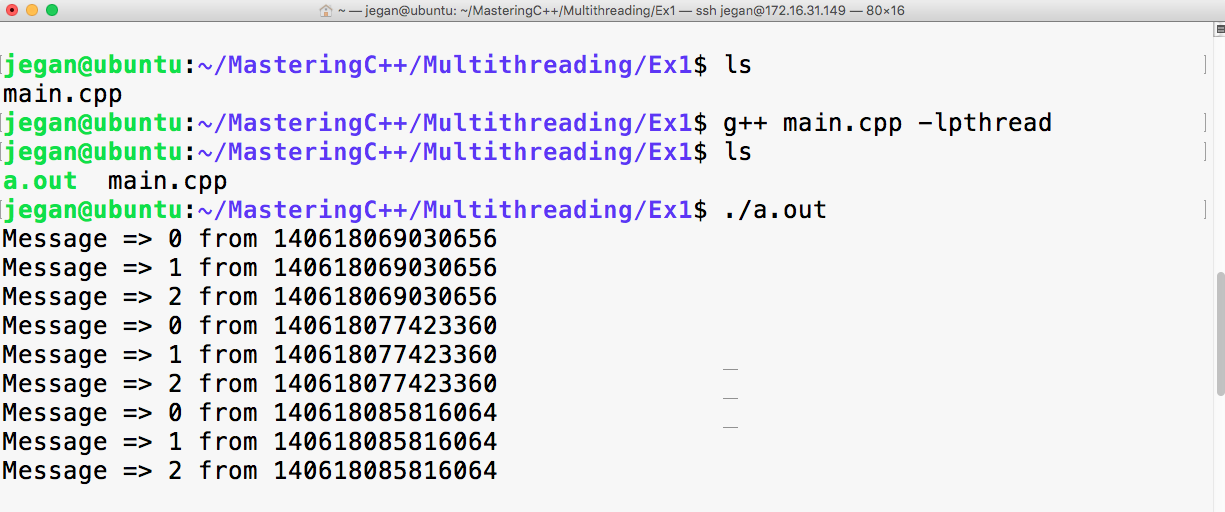
The code that is written in ThreadProc runs within the thread context. The preceding program has a total of four threads, including the main thread. I had blocked the main thread with pthread_join to force it to wait for the other three threads to complete their tasks first, failing which the main thread would have exited before them. When the main thread exits, the application exits too, which ends up prematurely destroying newly created threads.
Though we created thread1, thread2, and thread3 in the respective sequence, there is no guarantee that they will be started in the exact same sequence they were created in.
The operating system scheduler decides the sequence in which the threads must be started, based on the algorithm used by the operating system scheduler. Interestingly, the sequence in which the threads get started might vary at different runs in the same system.
Starting from C++11, C++ does support threads natively, and it is generally referred to as the C++ thread support library. The C++ thread support library provides an abstraction over the POSIX pthreads C library. Over time, C++ native thread support has improved to a greater extent.
I highly recommend you make use of the C++ native thread over pthreads. The C++ thread support library is supported on all platforms as it is officially part of standard C++ as opposed to the POSIX pthread library, which is only supported on Unix, Linux, and macOS but not directly on Windows.
The best part is thread support has matured to a new level in C++17, and it is poised to reach the next level in C++20. Hence, it is a good idea to consider using the C++ thread support library in your projects.
Essentially, to the operating system (OS), a process consists of one or more threads, each thread processing its own state and variables. One would regard this as a hierarchical configuration, with the OS as the foundation, providing support for the running of (user) processes. Each of these processes then consists of one or more threads. Communication between processes is handled by inter-process communication (IPC), which is provided by the operating system.
In a graphical view, this looks like the following:
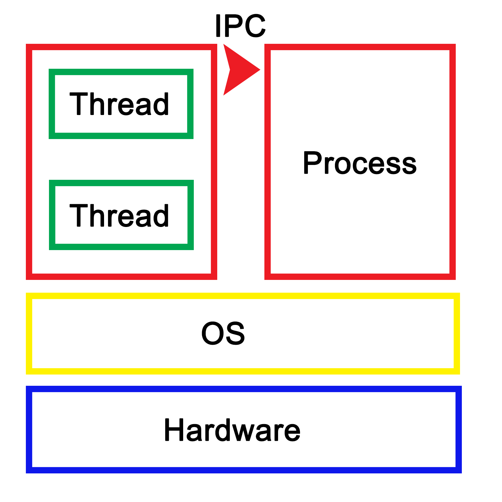
Each process within the OS has its own state, with each thread in a process having its own state as well as the relative to the other threads within that same process. While IPC allows processes to communicate with each other, threads can communicate with other threads within the process in a variety of ways, which we'll explore in more depth in upcoming chapters. This generally involves some kind of shared memory between threads.
An application is loaded from binary data in a specific executable format such as, for example, Executable and Linkable Format (ELF) which is generally used on Linux and many other operating systems. With ELF binaries, the following number of sections should always be present:
The .bss section is, essentially, allocated with uninitialized memory including empty arrays which thus do not take up any space in the binary, as it makes no sense to store rows of pure zeroes in the executable. Similarly, there is the .data section with initialized data. This contains global tables, variables, and the like. Finally, the .rodata section is like .data, but it is, as the name suggests, read-only. It contains things such as hardcoded strings.
In the .text section, we find the actual application instructions (code) which will be executed by the processor. The whole of this will get loaded by the operating system, thus creating a process. The layout of such a process looks like the following diagram:
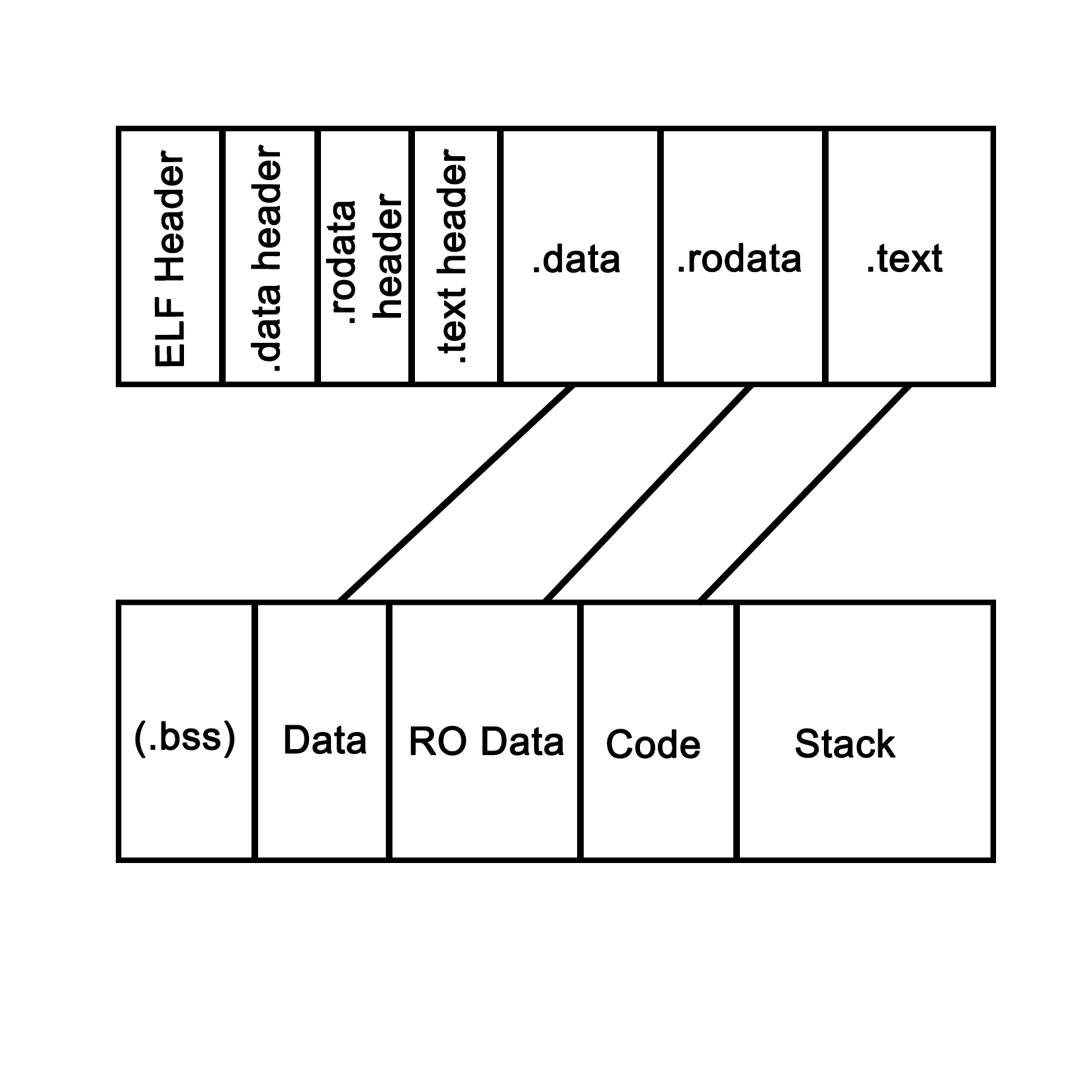
This is what a process looks like when launched from an ELF-format binary, though the final format in memory is roughly the same in basically any OS, including for a Windows process launched from a PE-format binary. Each of the sections in the binary are loaded into their respective sections, with the BSS section allocated to the specified size. The .text section is loaded along with the other sections, and its initial instruction is executed once this is done, which starts the process.
In system languages such as C++, one can see how variables and other program state information within such a process are stored both on the stack (variables exist within the scope) and heap (using the new operator). The stack is a section of memory (one allocated per thread), the size of which depends on the operating system and its configuration. One can generally also set the stack size programmatically when creating a new thread.
In an operating system, a process consists of a block of memory addresses, the size of which is constant and limited by the size of its memory pointers. For a 32-bit OS, this would limit this block to 4 GB. Within this virtual memory space, the OS allocates a basic stack and heap, both of which can grow until all memory addresses have been exhausted, and further attempts by the process to allocate more memory will be denied.
The stack is a concept both for the operating system and for the hardware. In essence, it's a collection (stack) of so-called stack frames, each of which is composed of variables, instructions, and other data relevant to the execution frame of a task.
In hardware terms, the stack is part of the task (x86) or process state (ARM), which is how the processor defines an execution instance (program or thread). This hardware-defined entity contains the entire state of a singular thread of execution. See the following sections for further details on this.
A task is defined as follows in the Intel IA-32 System Programming guide, Volume 3A:
"A task is a unit of work that a processor can dispatch, execute, and suspend. It can be used to execute a program, a task or process, an operating-system service utility, an interrupt or exception handler, or a kernel or executive utility."
"The IA-32 architecture provides a mechanism for saving the state of a task, for dispatching tasks for execution, and for switching from one task to another. When operating in protected mode, all processor execution takes place from within a task. Even simple systems must define at least one task. More complex systems can use the processor's task management facilities to support multitasking applications."
This excerpt from the IA-32 (Intel x86) manual summarizes how the hardware supports and implements support for operating systems, processes, and the switching between these processes.
It's important to realize here that, to the processor, there's no such thing as a process or thread. All it knows of are threads of execution, defined as a series of instructions. These instructions are loaded into memory somewhere, and the current position in these instructions is kept track of along with the variable data (variables) being created, as the application is executed within the data section of the process.
Each task also runs within a hardware-defined protection ring, with the OS's tasks generally running on ring 0, and user tasks on ring 3. Rings 1 and 2 are rarely used except for specific use cases with modern OSes on the x86 architecture. These rings are privilege-levels enforced by the hardware and allow for example for the strict separation of kernel and user-level tasks.
The task structure for both 32-bit and 64-bit tasks are quite similar in concept. The official name for it is the Task State Structure (TSS). It has the following layout for 32-bit x86 CPUs:
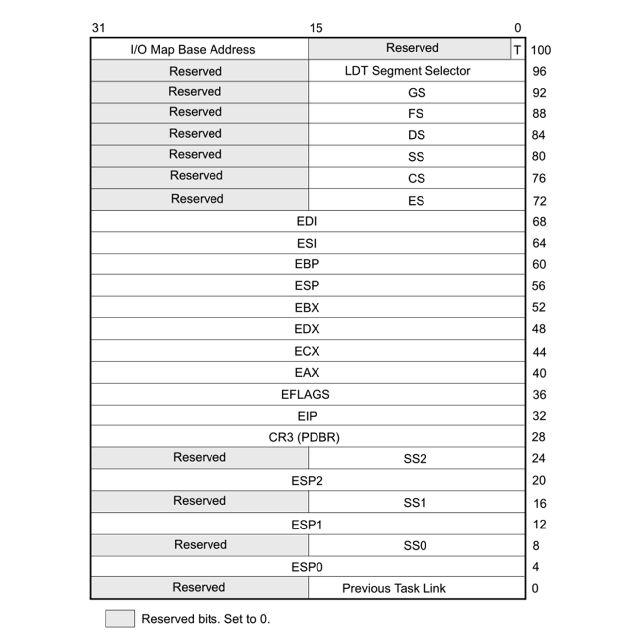
Following are the firlds:
For 64-bit x86_64 CPUs, the TSS layout looks somewhat different, since hardware-based task switching is not supported in this mode:
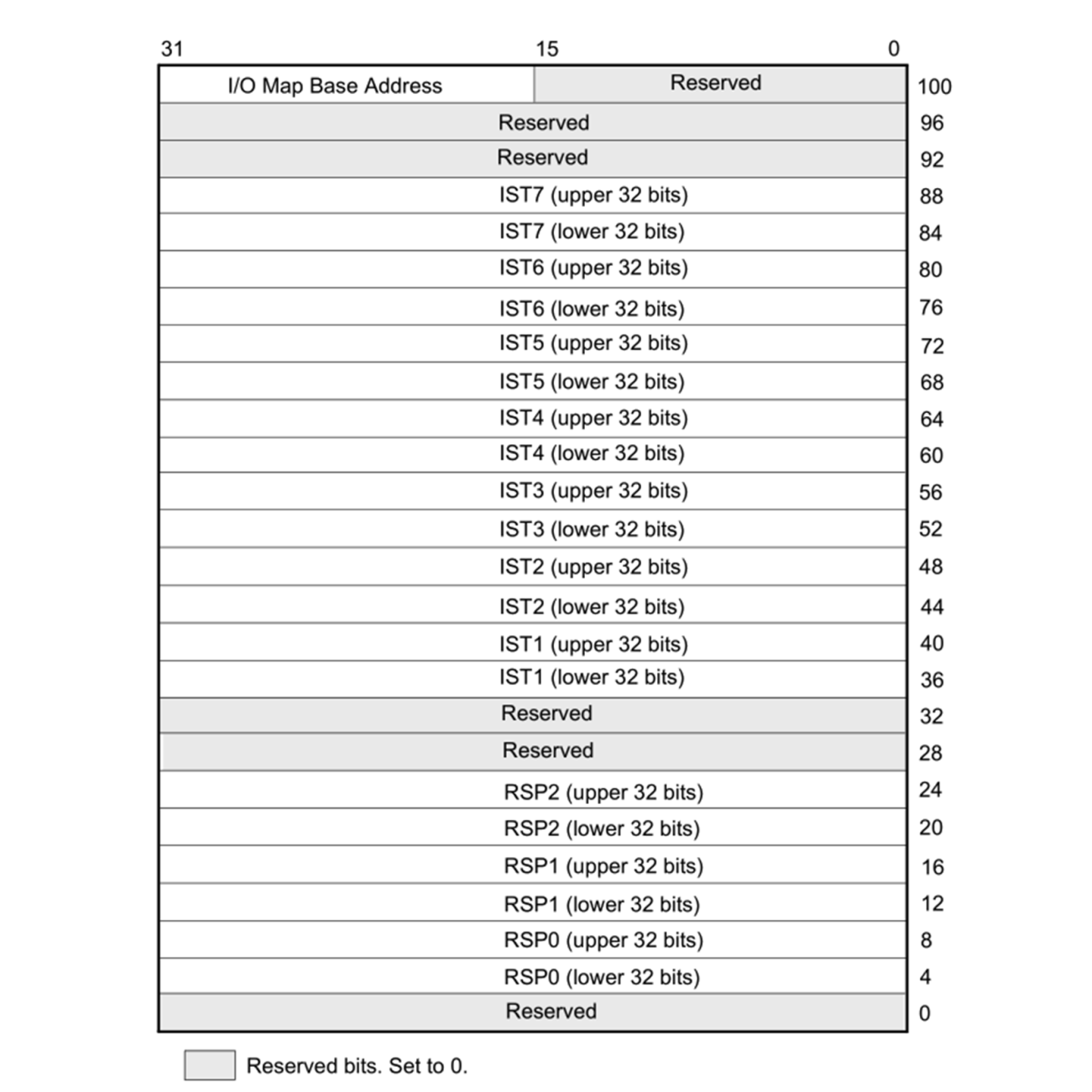
Here, we have similar relevant fields, just with different names:
Even though on x86 in 32-bit mode, the CPU supports hardware-based switching between tasks, most operating systems will use just a single TSS structure per CPU regardless of the mode, and do the actual switching between tasks in software. This is partially due to efficiency reasons (swapping out only pointers which change), partially due to features which are only possible this way, such as measuring CPU time used by a process/thread, and to adjust the priority of a thread or process. Doing it in software also simplifies the portability of code between 64-bit and 32-bit systems, since the former do not support hardware-based task switching.
During a software-based task switch (usually via an interrupt), the ESP/RSP, and so on are stored in memory and replaced with the values for the next scheduled task. This means that once execution resumes, the TSS structure will now have the Stack Pointer (SP), segment pointer(s), register contents, and all other details of the new task.
The source of the interrupt can be based in hardware or software. A hardware interrupt is usually used by devices to signal to the CPU that they require attention by the OS. The act of calling a hardware interrupt is called an Interrupt Request, or IRQ.
A software interrupt can be due to an exceptional condition in the CPU itself, or as a feature of the CPU's instruction set. The action of switching tasks by the OS's kernel is also performed by triggering a software interrupt.
In ARM architectures, applications usually run in the unprivileged Exception Level 0 (EL0) level, which is comparable to ring 3 on x86 architectures, and the OS kernel in EL1. The ARMv7 (AArch32, 32-bit) architecture has the SP in the general purpose register 13. For ARMv8 (AArch64, 64-bit), a dedicated SP register is implemented for each exception level: SP_EL0, SP_EL1, and so on.
For task state, the ARM architecture uses Program State Register (PSR) instances for the Current Program State Register (CPSR) or the Saved Program State Register (SPSR) program state's registers. The PSR is part of the Process State (PSTATE), which is an abstraction of the process state information.
While the ARM architecture is significantly different from the x86 architecture, when using software-based task switching, the basic principle does not change: save the current task's SP, register state, and put the next task's detail in there instead before resuming processing.
As we saw in the preceding sections, the stack together with the CPU registers define a task. As mentioned earlier, this stack consists of stack frames, each of which defines the (local) variables, parameters, data, and instructions for that particular instance of task execution. Of note is that although the stack and stack frames are primarily a software concept, it is an essential feature of any modern OS, with hardware support in many CPU instruction sets. Graphically, it can be be visualized like the following:
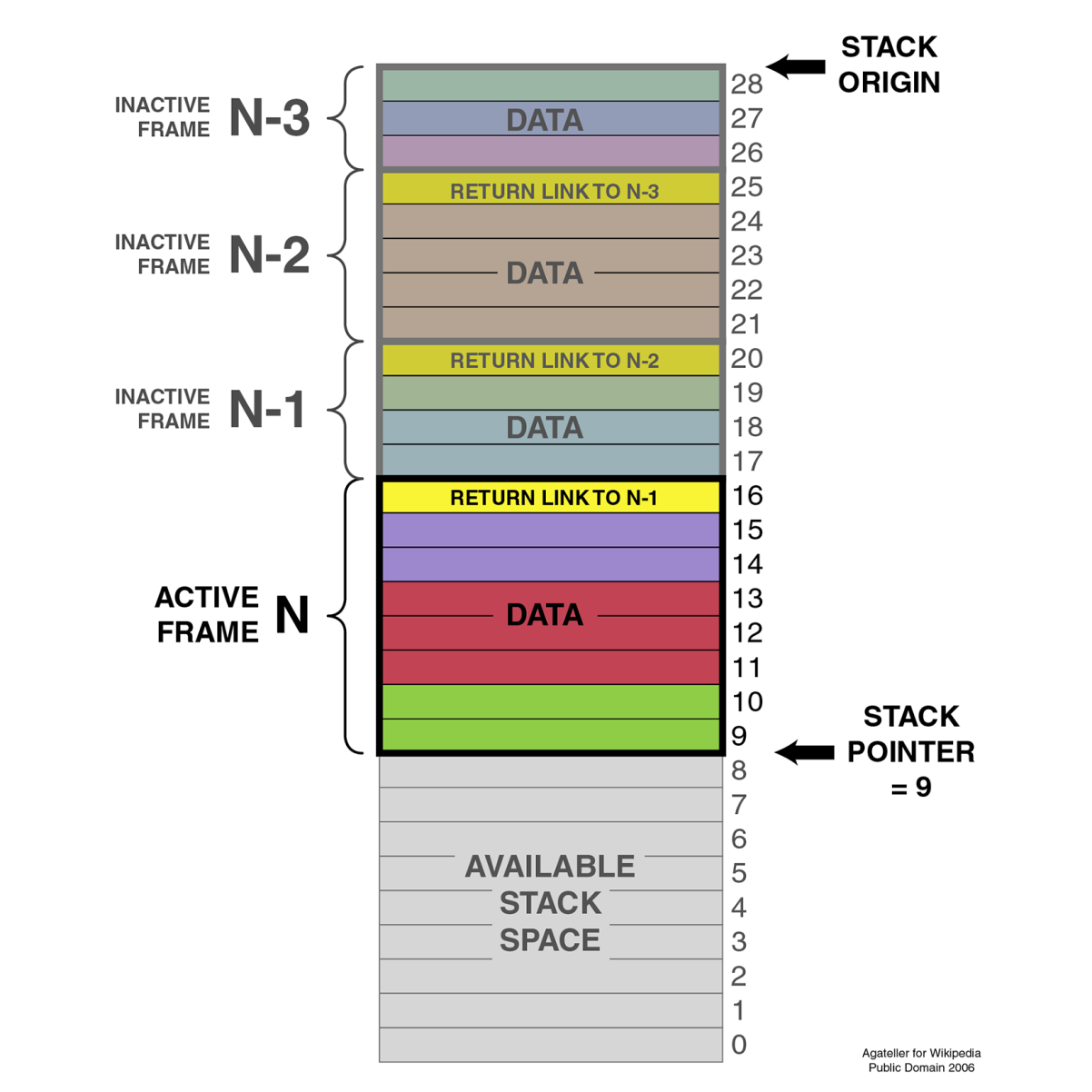
The SP (ESP on x86) points to the top of the stack, with another pointer (Extended Base Pointer (EBP) for x86). Each frame contains a reference to the preceding frame (caller return address), as set by the OS.
When using a debugger with one's C++ application, this is basically what one sees when requesting the backtrack--the individual frames of the stack showing the initial stack frame leading up until the current frame. Here, one can examine each individual frame's details.
Over the past decades, a lot of different terms related to the way tasks are processed by a computer have been coined and come into common use. Many of these are also used interchangeably, correctly or not. An example of this is multithreading in comparison with multiprocessing.
Here, the latter means running one task per processor in a system with multiple physical processors, while the former means running multiple tasks on a singular processor simultaneously, thus giving the illusion that they are all being executed simultaneously:
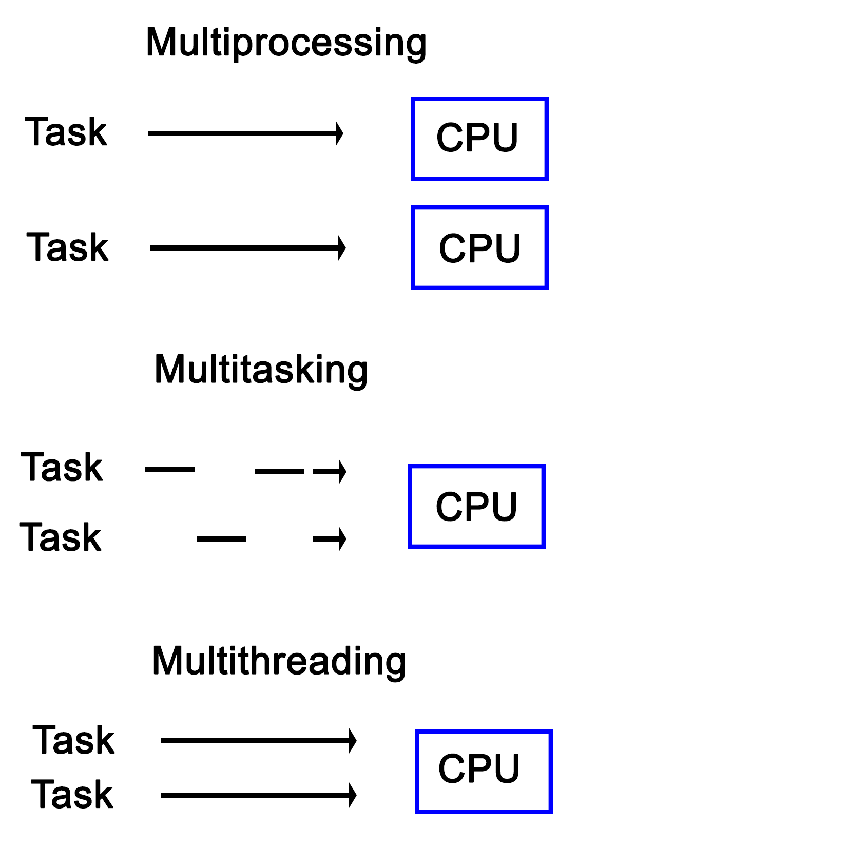
Another interesting distinction between multiprocessing and multitasking is that the latter uses time-slices in order to run multiple threads on a single processor core. This is different from multithreading in the sense that in a multitasking system, no tasks will ever run in a concurrent fashion on the same CPU core, though tasks can still be interrupted.
The concept of a process and a shared memory space between the threads contained within the said process is at the very core of multithreaded systems from a software perspective. Though the hardware is often not aware of this--seeing just a single task to the OS. However, such a multithreaded process contains two or many more threads. Each of these threads then perform its own series of tasks.
In other implementations, such as Intel's Hyper-Threading (HT) on x86 processors, this multithreading is implemented in the hardware itself, where it's commonly referred to as SMT (see the section Simultaneous multithreading (SMT) for details). When HT is enabled, each physical CPU core is presented to the OS as being two cores. The hardware itself will then attempt to execute the tasks assigned to these so-called virtual cores concurrently, scheduling operations which can use different elements of a processing core at the same time. In practice, this can give a noticeable boost in performance without the operating system or application requiring any type of optimization.
The OS can of course still do its own scheduling to further optimize the execution of task, since the hardware is not aware of many details about the instructions it is executing.
Having HT enabled looks like this in the visual format:
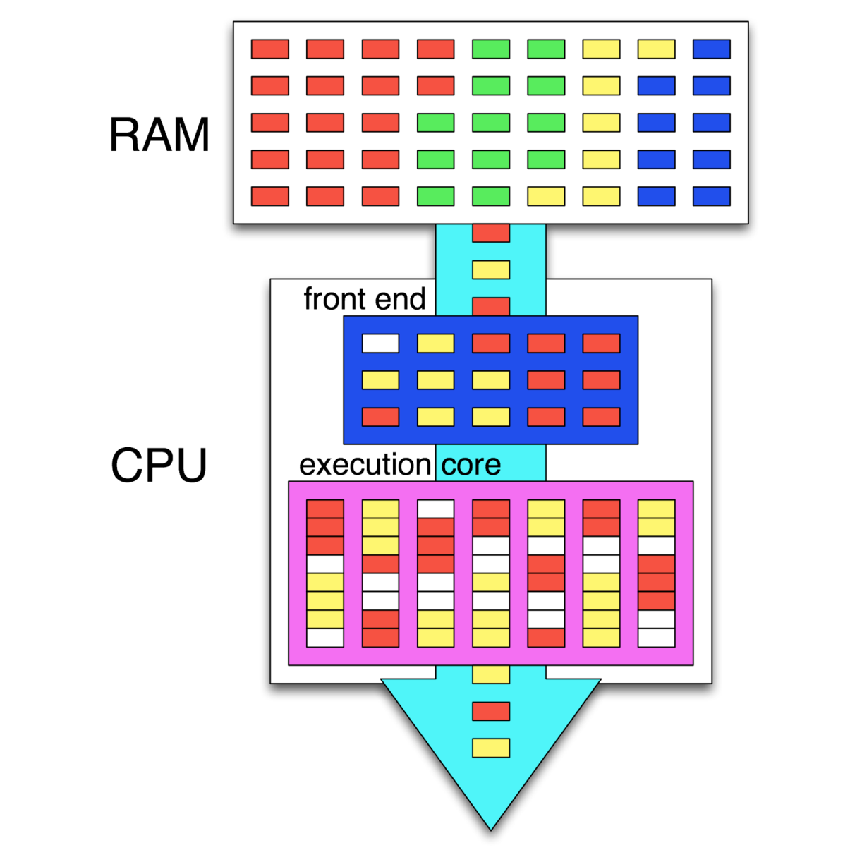
In this preceding graphic, we see the instructions of four different tasks in memory (RAM). Out of these, two tasks (threads) are being executed simultaneously, with the CPU's scheduler (in the frontend) attempting to schedule the instructions so that as many instructions as possible can be executed in parallel. Where this is not possible, so-called pipeline bubbles (in white) appear where the execution hardware is idle.
Together with internal CPU optimizations, this leads to a very high throughput of instructions, also called Instructions Per Second (IPC). Instead of the GHz rating of a CPU, this IPC number is generally far more significant for determining the sheer performance of a CPU.
Different types of computer architecture are classified using a system which was first proposed by Michael J. Flynn, back in 1966. This classification system knows four categories, defining the capabilities of the processing hardware in terms of the number of input and output streams:
An important thing to note with these categories is that they are all defined in terms of multiprocessing, meaning that they refer to the intrinsic capabilities of the hardware. Using software techniques, virtually any method can be approximated on even a regular SISD-style architecture. This is, however, part of multithreading.
Over the past decades, many systems were created which contained multiple processing units. These can be broadly divided into Symmetric Multiprocessing (SMP) and Asymmetric Multiprocessing (AMP) systems.
AMP's main defining feature is that a second processor is attached as a peripheral to the primary CPU. This means that it cannot run control software, but only user applications. This approach has also been used to connect CPUs using a different architecture to allow one to, for example, run x86 applications on an Amiga, 68k-based system.
With an SMP system, each of the CPUs are peers having access to the same hardware resources, and set up in a cooperative fashion. Initially, SMP systems involved multiple physical CPUs, but later, multiple processor cores got integrated on a single CPU die:
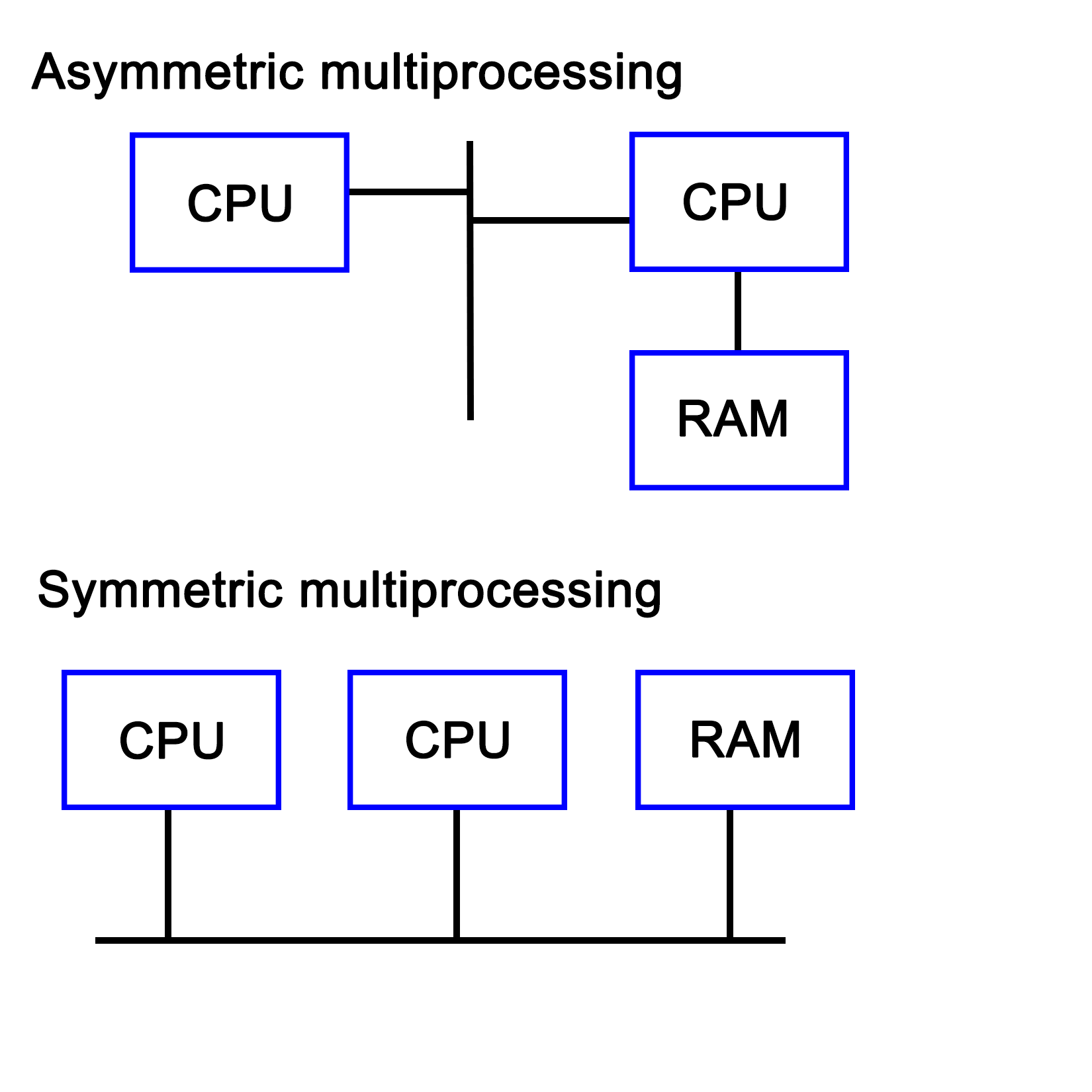
With the proliferation of multi-core CPUs, SMP is the most common type of processing outside of embedded development, where uniprocessing (single core, single processor) is still very common.
Technically, the sound, network, and graphic processors in a system can be considered to be asymmetric processors related to the CPU. With an increase in General Purpose GPU (GPGPU) processing, AMP is becoming more relevant.
A multiprocessing system does not necessarily have to be implemented within a single system, but can also consist of multiple systems which are connected in a network. Such a cluster is then called a loosely coupled multiprocessing system. We cover distributing computing in Chapter 9, Multithreading with Distributed Computing.
This is in contrast with a tightly coupled multiprocessing system, whereby the system is integrated on a single printed circuit board (PCB), using the same low-level, high-speed bus or similar.
Virtually any modern system combines multiprocessing with multithreading, courtesy of multi-core CPUs, which combine two or more processing cores on a single processor die. What this means for an operating system is that it has to schedule tasks both across multiple processing cores while also scheduling them on specific cores in order to extract maximum performance.
This is the area of task schedulers, which we will look at in a moment. Suffice it to say that this is a topic worthy of its own book.
Like multiprocessing, there is not a single implementation, but two main ones. The main distinction between these is the maximum number of threads the processor can execute concurrently during a single cycle. The main goal of a multithreading implementation is to get as close to 100% utilization of the processor hardware as reasonably possible. Multithreading utilizes both thread-level and process-level parallelism to accomplish this goal.
The are two types of multithreading, which we will cover in the following sections.
Also known as super-threading, the main subtypes for temporal multithreading (TMT) are coarse-grained and fine-grained (or interleaved). The former switches rapidly between different tasks, saving the context of each before switching to another task's context. The latter type switches tasks with each cycle, resulting in a CPU pipeline containing instructions from various tasks from which the term interleaved is derived.
The fine-grained type is implemented in barrel processors. They have an advantage over x86 and other architectures that they can guarantee specific timing (useful for hard real-time embedded systems) in addition to being less complex to implement due to assumptions that one can make.
SMT is implemented on superscalar CPUs (implementing instruction-level parallelism), which include the x86 and ARM architectures. The defining characteristic of SMT is also indicated by its name, specifically, its ability to execute multiple threads in parallel, per core.
Generally, two threads per core is common, but some designs support up to eight concurrent threads per core. The main advantage of this is being able to share resources among threads, with an obvious disadvantage of conflicting needs by multiple threads, which has to be managed. Another advantage is that it makes the resulting CPU more energy efficient due to a lack of hardware resource duplication.
Intel's HT technology is essentially Intel's SMT implementation, providing a basic two thread SMT engine starting with some Pentium 4 CPUs in 2002.
A number of task-scheduling algorithms exist, each focusing on a different goal. Some may seek to maximize throughput, others minimize latency, while others may seek to maximize response time. Which scheduler is the optimal choice solely depends on the application the system is being used for.
For desktop systems, the scheduler is generally kept as general-purpose as possible, usually prioritizing foreground applications over background applications in order to give the user the best possible desktop experience.
For embedded systems, especially in real-time, industrial applications would instead seek to guarantee timing. This allows processes to be executed at exactly the right time, which is crucial in, for example, driving machinery, robotics, or chemical processes where a delay of even a few milliseconds could be costly or even fatal.
The scheduler type is also dependent on the multitasking state of the OS--a cooperative multitasking system would not be able to provide many guarantees about when it can switch out a running process for another one, as this depends on when the active process yields.
With a preemptive scheduler, processes are switched without them being aware of it, allowing the scheduler more control over when processes run at which time points.
Windows NT-based OSes (Windows NT, 2000, XP, and so on) use what is called a multilevel feedback queue, featuring 32 priority levels. This type of priority scheduler allows one to prioritize tasks over other tasks, allowing one to fine-tune the resulting experience.
Linux originally (kernel 2.4) also used a multilevel feedback queue-based priority scheduler like Windows NT with an O(n) scheduler. With version 2.6, this was replaced with an O(1) scheduler, allowing processes to be scheduled within a constant amount of time. Starting with Linux kernel 2.6.23, the default scheduler is the Completely Fair Scheduler (CFS), which ensures that all tasks get a comparable share of CPU time.
The type of scheduling algorithm used for a number of commonly used or well-known OSes is listed in this table:
|
Operating System |
Preemption |
Algorithm |
|
Amiga OS |
Yes |
Prioritized round-robin scheduling |
|
FreeBSD |
Yes |
Multilevel feedback queue |
|
Linux kernel before 2.6.0 |
Yes |
Multilevel feedback queue |
|
Linux kernel 2.6.0-2.6.23 |
Yes |
O(1) scheduler |
|
Linux kernel after 2.6.23 |
Yes |
Completely Fair Scheduler |
|
classic Mac OS pre-9 |
None |
Cooperative scheduler |
|
Mac OS 9 |
Some |
Preemptive scheduler for MP tasks, and cooperative for processes and threads |
|
OS X/macOS |
Yes |
Multilevel feedback queue |
|
NetBSD |
Yes |
Multilevel feedback queue |
|
Solaris |
Yes |
Multilevel feedback queue |
|
Windows 3.1x |
None |
Cooperative scheduler |
|
Windows 95, 98, Me |
Half |
Preemptive scheduler for 32-bit processes, and cooperative for 16-bit processes |
|
Windows NT (including 2000, XP, Vista, 7, and Server) |
Yes |
Multilevel feedback queue |
(Source: https://en.wikipedia.org/wiki/Scheduling_(computing))
The preemptive column indicates whether the scheduler is preemptive or not, with the next column providing further details. As one can see, preemptive schedulers are very common, and used by all modern desktop operating systems.
In the demonstration code of Chapter 1, Revisiting Multithreading, we looked at a simple c++11 application which used four threads to perform some processing. In this section, we will look at the same application, but from a hardware and OS perspective.
When we look at the start of the code in the main function, we see that we create a data structure containing a single (integer) value:
int main() {
    values.push_back(42);
After the OS creates a new task and associated stack structure, an instance of a vector data structure (customized for integer types) is allocated on the stack. The size of this was specified in the binary file's global data section (BSS for ELF).
When the application's execution is started using its entry function (main() by default), the data structure is modified to contain the new integer value.
Next, we create four threads, providing each with some initial data:
thread tr1(threadFnc, 1);
thread tr2(threadFnc, 2);
thread tr3(threadFnc, 3);
thread tr4(threadFnc, 4);
For the OS, this means creating new data structures, and allocating a stack for each new thread. For the hardware, this initially does not change anything if no hardware-based task switching is used.
At this point, the OS's scheduler and the CPU can combine to execute this set of tasks (threads) as efficiently and quickly as possible, employing features of the hardware including SMP, SMT, and so on.
After this, the main thread waits until the other threads stop executing:
tr1.join();
tr2.join();
tr3.join();
tr4.join();
These are blocking calls, which mark the main thread as being blocked until these four threads (tasks) finish executing. At this point, the OS's scheduler will resume execution of the main thread.
In each newly created thread, we first output a string on the standard output, making sure that we lock the mutex to ensure synchronous access:
void threadFnc(int tid) {
cout_mtx.lock();
cout << "Starting thread " << tid << ".n";
cout_mtx.unlock();
A mutex, in essence, is a singular value being stored on the stack of heap, which then is accessed using an atomic operation. This means that some form of hardware support is required. Using this, a task can check whether it is allowed to proceed yet, or has to wait and try again.
In this last particular piece of code, this mutex lock allows us to output on the standard C++ output stream without other threads interfering.
After this, we copy the initial value in the vector to a local variable, again ensuring that it's done synchronously:
values_mtx.lock();
int val = values[0];
values_mtx.unlock();
The same thing happens here, except now the mutex lock allows us to read the first value in the vector without risking another thread accessing or even changing it while we use it.
This is followed by the generating of a random number as follows:
int rval = randGen(0, 10);
val += rval;
This uses the randGen() method, which is as follows:
int randGen(const int& min, const int& max) {
static thread_local mt19937 generator(hash<thread::id>() (this_thread::get_id()));
uniform_int_distribution<int> distribution(min, max);
return distribution(generator);
}
This method is interesting due to its use of a thread-local variable. Thread-local storage is a section of a thread's memory which is specific to it, and used for global variables, which, nevertheless, have to remain limited to that specific thread.
This is very useful for a static variable like the one used here. That the generator instance is static is because we do not want to reinitialize it every single time we use this method, yet we do not want to share this instance across all threads. By using a thread-local, static instance, we can accomplish both goals. A static instance is created and used, but separately for each thread.
The Thread function then ends with the same series of mutexes being locked, and the new value being copied to the array.
cout_mtx.lock();
cout << "Thread " << tid << " adding " << rval << ". New value: " << val << ".n";
cout_mtx.unlock();
values_mtx.lock();
values.push_back(val);
values_mtx.unlock();
}
Here we see the same synchronous access to the standard output stream, followed by synchronous access to the values data structure.
Mutual exclusion is the principle which underlies thread-safe access of data within a multithreaded application. One can implement this both in hardware and software. The mutual exclusion (mutex) is the most elementary form of this functionality in most implementations.
The simplest hardware-based implementation on a uniprocessor (single processor core), non-SMT system is to disable interrupts, and thus, prevent the task from being changed. More commonly, a so-called busy-wait principle is employed. This is the basic principle behind a mutex--due to how the processor fetches data, only one task can obtain and read/write an atomic value in the shared memory, meaning, a variable sized the same (or smaller) as the CPU's registers. This is further detailed in Chapter 15, Atomic Operations - Working with the Hardware.
When our code tries to lock a mutex, what this does is read the value of such an atomic section of memory, and try to set it to its locked value. Since this is a single operation, only one task can change the value at any given time. Other tasks will have to wait until they can gain access in this busy-wait cycle, as shown in this diagram:
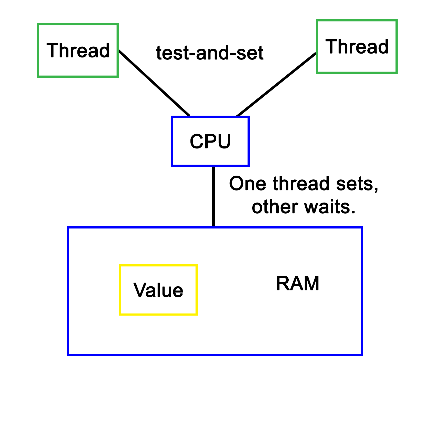
Software-defined mutual exclusion implementations are all based on busy-waiting. An example is Dekker's algorithm, which defines a system in which two processes can synchronize, employing busy-wait to wait for the other process to leave the critical section.
The pseudocode for this algorithm is as follows:
variables
wants_to_enter : array of 2 booleans
turn : integer
wants_to_enter[0] ← false
wants_to_enter[1] ← false
turn ← 0 // or 1
p0:
wants_to_enter[0] ← true
while wants_to_enter[1] {
if turn ≠ 0 {
wants_to_enter[0] ← false
while turn ≠ 0 {
// busy wait
}
wants_to_enter[0] ← true
}
}
// critical section
...
turn ← 1
wants_to_enter[0] ← false
// remainder section
p1:
wants_to_enter[1] ← true
while wants_to_enter[0] {
if turn ≠ 1 {
wants_to_enter[1] ← false
while turn ≠ 1 {
// busy wait
}
wants_to_enter[1] ← true
}
}
// critical section
...
turn ← 0
wants_to_enter[1] ← false
// remainder section
(Referenced from: https://en.wikipedia.org/wiki/Dekker's_algorithm)
In this preceding algorithm, processes indicate the intent to enter a critical section, checking whether it's their turn (using the process ID), then setting their intent to enter the section to false after they have entered it. Only once a process has set its intent to enter to true again will it enter the critical section again. If it wishes to enter, but turn does not match its process ID, it'll busy-wait until the condition becomes true.
A major disadvantage of software-based mutual exclusion algorithms is that they only work if out-of-order (OoO) execution of code is disabled. OoO means that the hardware actively reorders incoming instructions in order to optimize their execution, thus changing their order. Since these algorithms require that various steps are executed in order, they no longer work on OoO processors.
Every modern programming language supports concurrency, offering high-level APIs that allow the execution of many tasks simultaneously. C++ supports concurrency starting from C++11 and more sophisticated APIs got added further in C++14 and C++17. Though the C++ thread support library allows multithreading, it requires writing lengthy code using complex synchronizations; however, concurrency lets us execute independent tasks--even loop iterations can run concurrently without writing complex code. The bottom line is parallelization is made more easy with concurrency.
The concurrency support library complements the C++ thread support library. The combined use of these two powerful libraries makes concurrent programming more easy in C++.
Let's write a simple Hello World program using C++ concurrency in the following file named main.cpp:
#include <iostream>
#include <future>
using namespace std;
void sayHello( ) {
cout << endl << "Hello Concurrency support library!" << endl;
}
int main ( ) {
future<void> futureObj = async ( launch::async, sayHello );
futureObj.wait( );
return 0;
}
Let's try to understand the main() function. Future is an object of the concurrency module that helps the caller function retrieve the message passed by the thread in an asynchronous fashion. The void in future<void> represents the sayHello() thread function that is not expected to pass any message to the caller, that is, the main thread function. The async class lets us execute a function in two modes, namely launch::async or launch::deferred mode.
The launch::async mode lets the async object launch the sayHello() method in a separate thread, whereas the launch::deferred mode lets the async object invoke the sayHello() function without creating a separate thread. In launch::deferred mode, the sayHello() method invocation will be different until the caller thread invokes the future::get() method.
The futureObj.wait() voice is used to block the main thread to let the sayHello() function complete its task. The future::wait() function is similar to thread::join() in the thread support library.
Let's go ahead and compile the program with the following command:
g++ main.cpp -o concurrency.exe -std=c++17 -lpthread
Let's launch concurrency.exe, as shown ahead, and understand how it works:
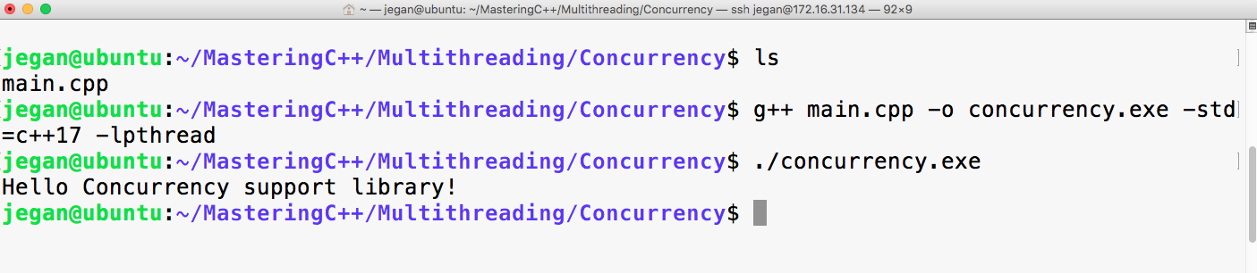
Let's slightly modify main.cpp, the Hello World program we wrote in the previous section. Let's understand how we could pass a message from a Thread function to the caller function asynchronously:
#include <iostream>
#include <future>
using namespace std;
void sayHello( promise<string> promise_ ) {
promise_.set_value ( "Hello Concurrency support library!" );
}
int main ( ) {
promise<string> promiseObj;
future<string> futureObj = promiseObj.get_future( );
async ( launch::async, sayHello, move( promiseObj ) );
cout << futureObj.get( ) << endl;
return 0;
}
In the previous program, promiseObj is used by the sayHello() thread function to pass the message to the main thread asynchronously. Note that promise<string> implies that the sayHello() function is expected to pass a string message, hence the main thread retrieves future<string>. The future::get() function call will be blocked until the sayHello() thread function calls the promise::set_value() method.
However, it is important to understand that future::get() must only be called once as the corresponding promise object will be destructed after the call to the future::get() method invocation.
Did you notice the use of the std::move() function? The std::move() function basically transfers the ownership of promiseObj to the sayHello() thread function, hence promiseObj must not be accessed from the main thread after std::move() is invoked.
Let's go ahead and compile the program with the following command:
g++ main.cpp -o concurrency.exe -std=c++17 -lpthread
Observe how the concurrency.exe application works by launching concurrency.exe as shown ahead:

As you may have guessed, the output of this program is exactly the same as our previous version. But this version of our program makes use of promise and future objects, unlike the previous version that doesn't support message passing.
The concurrency support module supports a concept called task. A task is work that happens concurrently across threads. A concurrent task can be created using the packaged_task class. The packaged_task class conveniently connects the thread function, the corresponding promise, and feature objects.
Let's understand the use of packaged_task with a simple example. The following program gives us an opportunity to taste a bit of functional programming with lambda expressions and functions:
#include <iostream>
#include <future>
#include <promise>
#include <thread>
#include <functional>
using namespace std;
int main ( ) {
packaged_task<int (int, int)>
addTask ( [] ( int firstInput, int secondInput ) {
return firstInput + secondInput;
} );
future<int> output = addTask.get_future( );
addTask ( 15, 10 );
cout << "The sum of 15 + 10 is " << output.get() << endl;
return 0;
}
In the previously shown program, I created a packaged_task instance called addTask. The packaged_task< int (int,int)> instance implies that the add task will return an integer and take two integer arguments:
addTask ( [] ( int firstInput, int secondInput ) {
return firstInput + secondInput;
});
The preceding code snippet indicates it is a lambda function that is defined anonymously.
The interesting part is that the addTask( ) call in main.cpp appears like a regular function call. The future<int> object is extracted from the packaged_task instance addTask, which is then used to retrieve the output of the addTask via the future object instance, that is, the get() method.
Let's go ahead and compile the program with the following command:
g++ main.cpp -o concurrency.exe -std=c++17 -lpthread
Let's quickly launch concurrency.exe and observe the output shown next:

Cool! You learned how to use lambda functions with the concurrency support library.
In the previous section, you learned how packaged_task can be used in an elegant way. I love lambda functions a lot. They look a lot like mathematics. But not everyone likes lambda functions as they degrade readability to some extent. Hence, it isn't mandatory to use lambda functions with a concurrent task if you don't prefer lambdas. In this section, you'll understand how to use a concurrent task with the thread support library, as shown in the following code:
#include <iostream>
#include <future>
#include <thread>
#include <functional>
using namespace std;
int add ( int firstInput, int secondInput ) {
return firstInput + secondInput;
}
int main ( ) {
packaged_task<int (int, int)> addTask( add);
future<int> output = addTask.get_future( );
thread addThread ( move(addTask), 15, 10 );
addThread.join( );
cout << "The sum of 15 + 10 is " << output.get() << endl;
return 0;
}
Let's go ahead and compile the program with the following command:
g++ main.cpp -o concurrency.exe -std=c++17 -lpthread
Let's launch concurrency.exe, as shown in the following screenshot, and understand the difference between the previous program and the current version:

Yes, the output is the same as the previous section because we just refactored the code.
Wonderful! You just learned how to integrate the C++ thread support library with concurrent components.
In this section, you will learn how you can bind the thread function and its respective arguments with packaged_task.
Let's take the code from the previous section and modify it to understand the bind feature, as follows:
#include <iostream>
#include <future>
#include <string>
using namespace std;
int add ( int firstInput, int secondInput ) {
return firstInput + secondInput;
}
int main ( ) {
packaged_task<int (int,int)> addTask( add );
future<int> output = addTask.get_future();
thread addThread ( move(addTask), 15, 10);
addThread.join();
cout << "The sum of 15 + 10 is " << output.get() << endl;
return 0;
}
The std::bind( ) function binds the thread function and its arguments with the respective task. Since the arguments are bound upfront, there is no need to supply the input arguments 15 or 10 once again. These are some of the convenient ways in which packaged_task can be used in C++.
Let's go ahead and compile the program with the following command:
g++ main.cpp -o concurrency.exe -std=c++17 -lpthread
Let's launch concurrency.exe, as shown in the following screenshot, and understand the difference between the previous program and the current version:
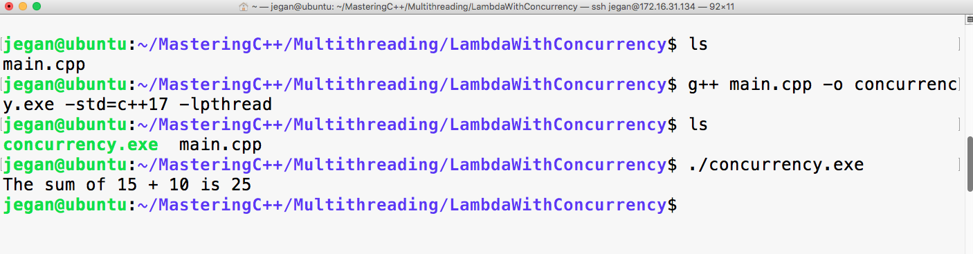
Congrats! You have learned a lot about concurrency in C++ so far.
The concurrency support library also supports passing exceptions via a future object.
Let's understand the exception concurrency handling mechanism with a simple example, as follows:
#include <iostream>
#include <future>
#include <promise>
using namespace std;
void add ( int firstInput, int secondInput, promise<int> output ) {
try {
if ( ( INT_MAX == firstInput ) || ( INT_MAX == secondInput ) )
output.set_exception( current_exception() ) ;
}
catch(...) {}
output.set_value( firstInput + secondInput ) ;
}
int main ( ) {
try {
promise<int> promise_;
future<int> output = promise_.get_future();
async ( launch::deferred, add, INT_MAX, INT_MAX, move(promise_) );
cout << "The sum of INT_MAX + INT_MAX is " << output.get ( ) << endl;
}
catch( exception e ) {
cerr << "Exception occured" << endl;
}
}
Just like the way we passed the output messages to the caller function/thread, the concurrency support library also allows you to set the exception that occurred within the task or asynchronous function. When the caller thread invokes the future::get() method, the same exception will be thrown, hence communicating exceptions is made easy.
Let's go ahead and compile the program with the following command. Uncle fruits and yodas malte:
g++ main.cpp -o concurrency.exe -std=c++17 -lpthread
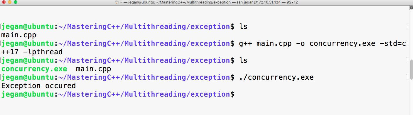
Let me summarize the takeaway points:
In this chapter, we saw how processes and threads are implemented both in operating systems and in hardware. We also looked at various configurations of processor hardware and elements of operating systems involved in scheduling to see how they provide various types of task processing.
Finally, we took the multithreaded program example of the previous chapter, and ran through it again, this time considering what happens in the OS and processor while it is being executed.
In the next chapter, we will take a look at the various multithreading APIs being offered via OS and library-based implementations, along with examples comparing these APIs.
While C++ has a native multithreading implementation in the Standard Template Library (STL), OS-level and framework-based multithreading APIs are still very common. Examples of these APIs include Windows and POSIX (Portable Operating System Interface) threads, and those provided by the Qt, Boost, and POCO libraries.
This chapter takes a detailed look at the features provided by each of these APIs, as well as the similarities and differences between each of them. Finally, we'll look at common usage scenarios using example code.
Topics covered by this chapter include the following:
Before the C++ 2011 (C++11) standard, many different threading implementations were developed, many of which are limited to a specific software platform. Some of these are still relevant today, such as Windows threads. Others have been superseded by standards, of which POSIX Threads (Pthreads) has become the de facto standard on UNIX-like OSes. This includes Linux-based and BSD-based OS, as well as OS X (macOS) and Solaris.
Many libraries were developed to make cross-platform development easier. Although Pthreads helps to make UNIX-like OS more or less compatible one of the prerequisites to make software portable across all major operating systems, a generic threading API is needed. This is why libraries such as Boost, POCO, and Qt were created. Applications can use these and rely on the library to handle any differences between platforms.
Pthreads were first defined in the POSIX.1c standard (Threads extensions, IEEE Std 1003.1c-1995) from 1995 as an extension to the POSIX standard. At the time, UNIX had been chosen as a manufacturer-neutral interface, with POSIX unifying the various APIs among them.
Despite this standardization effort, differences still exist in Pthread implementations between OS's which implement it (for example, between Linux and OS X), courtesy of non-portable extensions (marked with _np in the method name).
For the pthread_setname_np method, the Linux implementation takes two parameters, allowing one to set the name of a thread other than the current thread. On OS X (since 10.6), this method only takes one parameter, allowing one to set the name of the current thread only. If portability is a concern, one has to be mindful of such differences.
After 1997, the POSIX standard revisions were managed by the Austin Joint Working Group. These revisions merge the threads extension into the main standard. The current revision is 7, also known as POSIX.1-2008 and IEEE Std 1003.1, 2013 edition--with a free copy of the standard available online.
OS's can be certified to conform to the POSIX standard. Currently, these are as mentioned in this table:
| Name | Developer | Since version | Architecture(s) (current) | Notes |
|
AIX |
IBM |
5L |
POWER |
Server OS |
|
HP-UX |
Hewlett-Packard |
11i v3 |
PA-RISC, IA-64 (Itanium) |
Server OS |
|
IRIX |
Silicon Graphics (SGI) |
6 |
MIPS |
Discontinued |
|
Inspur K-UX |
Inspur |
2 |
X86_64, |
Linux based |
|
Integrity |
Green Hills Software |
5 |
ARM, XScale, Blackfin, Freescale Coldfire, MIPS, PowerPC, x86. |
Real-time OS |
|
OS X/MacOS |
Apple |
10.5 (Leopard) |
X86_64 |
Desktop OS |
|
QNX Neutrino |
BlackBerry |
1 |
Intel 8088, x86, MIPS, PowerPC, SH-4, ARM, StrongARM, XScale |
Real-time, embedded OS |
|
Solaris |
Sun/Oracle |
2.5 |
SPARC, IA-32 (<11), x86_64, PowerPC (2.5.1) |
Server OS |
|
Tru64 |
DEC, HP, IBM, Compaq |
5.1B-4 |
Alpha |
Discontinued |
|
UnixWare |
Novell, SCO, Xinuos |
7.1.3 |
x86 |
Server OS |
Other operating systems are mostly compliant. The following are examples of the same:
| Name | Platform | Notes |
|
Android |
ARM, x86, MIPS |
Linux based. Bionic C-library. |
|
BeOS (Haiku) |
IA-32, ARM, x64_64 |
Limited to GCC 2.x for x86. |
|
Darwin |
PowerPC, x86, ARM |
Uses the open source components on which macOS is based. |
|
FreeBSD |
IA-32, x86_64, sparc64, PowerPC, ARM, MIPS, and so on |
Essentially POSIX compliant. One can rely on documented POSIX behavior. More strict on compliance than Linux, in general. |
|
Linux |
Alpha, ARC, ARM, AVR32, Blackfin, H8/300, Itanium, m68k, Microblaze, MIPS, Nios II, OpenRISC, PA-RISC, PowerPC, s390, S+core, SuperH, SPARC, x86, Xtensa, and so on |
Some Linux distributions (see previous table) are certified as being POSIX compliant. This does not imply that every Linux distribution is POSIX compliant. Some tools and libraries may differ from the standard. For Pthreads, this may mean that the behavior is sometimes different between Linux distributions (different scheduler, and so on) as well as compared to other OS's implementing Pthreads. |
|
MINIX 3 |
IA-32, ARM |
Conforms to POSIX specification standard 3 (SUSv3, 2004). |
|
NetBSD |
Alpha, ARM, PA-RISC, 68k, MIPS, PowerPC, SH3, SPARC, RISC-V, VAX, x86, and so on |
Almost fully compatible with POSX.1 (1990), and mostly compliant with POSIX.2 (1992). |
|
Nuclear RTOS |
ARM, MIPS, PowerPC, Nios II, MicroBlaze, SuperH, and so on |
Proprietary RTOS from Mentor Graphics aimed at embedded applications. |
|
NuttX |
ARM, AVR, AVR32, HCS12, SuperH, Z80, and so on |
Light-weight RTOS, scalable from 8 to 32-bit systems with strong focus on POSIX compliance. |
|
OpenBSD |
Alpha, x86_64, ARM, PA-RISC, IA-32, MIPS, PowerPC, SPARC, and so on |
Forked from NetBSD in 1995. Similar POSIX support. |
|
OpenSolaris/illumos |
IA-32, x86_64, SPARC, ARM |
Compliant with the commercial Solaris releases being certified compatible. |
|
VxWorks |
ARM, SH-4, x86, x86_64, MIPS, PowerPC |
POSIX compliant, with certification for user-mode execution environment. |
From this it should be obvious that it's not a clear matter of following the POSIX specification, and being able to count on one's code compiling on each of these platforms. Each platform will also have its own set of extensions to the standard for features which were omitted in the standard, but are still desirable. Pthreads are, however, widely used by Linux, BSD, and similar software.
It's also possible to use the POSIX APIs in a limited fashion using, for example, the following:
| Name | Compliance |
|
Cygwin |
Mostly complete. Provides a full runtime environment for a POSIX application, which can be distributed as a normal Windows application. |
|
MinGW |
With MinGW-w64 (a redevelopment of MinGW), Pthreads support is fairly complete, though some functionality may be absent. |
|
Windows Subsystem for Linux |
WSL is a Windows 10 feature, which allows a Ubuntu Linux 14.04 (64-bit) image's tools and utilities to run natively on top of it though not those using GUI features or missing kernel features. Otherwise, it offers similar compliance as Linux. This feature currently requires that one runs the Windows 10 Anniversary Update and install WSL by hand using instructions provided by Microsoft. |
POSIX on Windows is generally not recommended. Unless there are good reasons to use POSIX (large existing code base, for example), it's far easier to use one of the cross-platform APIs (covered later in this chapter), which smooth away any platform issues.
In the following sections, we'll look at the features offered by the Pthreads API.
These are all the functions which start with either pthread_ or pthread_attr_. These functions all apply to threads themselves and their attribute objects.
The basic use of threads with Pthreads looks like the following:
#include <pthread.h>
#include <stdlib.h>
#define NUM_THREADS 5
The main Pthreads header is pthread.h. This gives access to everything but semaphores (covered later in this section). We also define a constant for the number of threads we wish to start here:
void* worker(void* arg) {
int value = *((int*) arg);
// More business logic.
return 0;
}
We define a simple Worker function, which we'll pass to the new thread in a moment. For demonstration and debugging purposes one could first add a simple cout or printf-based bit of business logic to print out the value sent to the new thread.
Next, we define the main function as follows:
int main(int argc, char** argv) {
pthread_t threads[NUM_THREADS];
int thread_args[NUM_THREADS];
int result_code;
for (unsigned int i = 0; i < NUM_THREADS; ++i) {
thread_args[i] = i;
result_code = pthread_create(&threads[i], 0, worker, (void*) &thread_args[i]);
}
We create all of the threads in a loop in the preceding function. Each thread instance gets a thread ID assigned (first argument) when created in addition to a result code (zero on success) returned by the pthread_create() function. The thread ID is the handle to reference the thread in future calls.
The second argument to the function is a pthread_attr_t structure instance, or 0 if none. This allows for configuration characteristics of the new thread, such as the initial stack size. When zero is passed, default parameters are used, which differ per platform and configuration.
The third parameter is a pointer to the function which the new thread will start with. This function pointer is defined as a function which returns a pointer to void data (that is, custom data), and accepts a pointer to void data. Here, the data being passed to the new thread as an argument is the thread ID:
for (int i = 0; i < NUM_THREADS; ++i) {
result_code = pthread_join(threads[i], 0);
}
exit(0);
}
Next, we wait for each worker thread to finish using the pthread_join() function. This function takes two parameters, the ID of the thread to wait for, and a buffer for the return value of the Worker function (or zero).
Other functions to manage threads are as follows:
Beyond this, there are the pthread_attr_* functions to manipulate and obtain information about a pthread_attr_t structure.
These are functions prefixed with either pthread_mutex_ or pthread_mutexattr_. They apply to mutexes and their attribute objects.
Mutexes in Pthreads can be initialized, destroyed, locked, and unlocked. They can also have their behavior customized using a pthread_mutexattr_t structure, which has its corresponding pthread_mutexattr_* functions for initializing and destroying an attribute on it.
A basic use of a Pthread mutex using static initialization looks as follows:
static pthread_mutex_t func_mutex = PTHREAD_MUTEX_INITIALIZER;
void func() {
pthread_mutex_lock(&func_mutex);
// Do something that's not thread-safe.
pthread_mutex_unlock(&func_mutex);
}
In this last bit of code, we use the PTHREAD_MUTEX_INITIALIZER macro, which initializes the mutex for us without having to type out the code for it every time. In comparison to other APIs, one has to manually initialize and destroy mutexes, though the use of macros helps somewhat.
After this, we lock and unlock the mutex. There's also the pthread_mutex_trylock() function, which is like the regular lock version, but which will return immediately if the referenced mutex is already locked instead of waiting for it to be unlocked.
In this example, the mutex is not explicitly destroyed. This is, however, a part of normal memory management in a Pthreads-based application.
These are functions which are prefixed with either pthread_cond_ or pthread_condattr_. They apply to condition variables and their attribute objects.
Condition variables in Pthreads follow the same pattern of having an initialization and a destroy function in addition to having the same for managing a pthread_condattr_t attribution structure.
This example covers basic usage of Pthreads condition variables:
#include <pthread.h>
#include <stdlib.h>
#include <unistd.h>
#define COUNT_TRIGGER 10
#define COUNT_LIMIT 12
int count = 0;
int thread_ids[3] = {0,1,2};
pthread_mutex_t count_mutex;
pthread_cond_t count_cv;
In the preceding code, we get the standard headers, and define a count trigger and limit, whose purpose will become clear in a moment. We also define a few global variables: a count variable, the IDs for the threads we wish to create, as well as a mutex and condition variable:
void* add_count(void* t) {
int tid = (long) t;
for (int i = 0; i < COUNT_TRIGGER; ++i) {
pthread_mutex_lock(&count_mutex);
count++;
if (count == COUNT_LIMIT) {
pthread_cond_signal(&count_cv);
}
pthread_mutex_unlock(&count_mutex);
sleep(1);
}
pthread_exit(0);
}
This preceding function, essentially, just adds to the global counter variable after obtaining exclusive access to it with the count_mutex. It also checks whether the count trigger value has been reached. If it has, it will signal the condition variable.
To give the second thread, which also runs this function, a chance to get the mutex, we sleep for 1 second in each cycle of the loop:
void* watch_count(void* t) {
int tid = (int) t;
pthread_mutex_lock(&count_mutex);
if (count < COUNT_LIMIT) {
pthread_cond_wait(&count_cv, &count_mutex);
}
pthread_mutex_unlock(&count_mutex);
pthread_exit(0);
}
In this second function, we lock the global mutex before checking whether we have reached the count limit yet. This is our insurance in case the thread running this function does not get called before the count reaches the limit.
Otherwise, we wait on the condition variable providing the condition variable and locked mutex. Once signaled, we unlock the global mutex, and exit the thread.
A point to note here is that this example does not account for spurious wake-ups. Pthreads condition variables are susceptible to such wake-ups which necessitate one to use a loop and check whether some kind of condition has been met:
int main (int argc, char* argv[]) {
int tid1 = 1, tid2 = 2, tid3 = 3;
pthread_t threads[3];
pthread_attr_t attr;
pthread_mutex_init(&count_mutex, 0);
pthread_cond_init (&count_cv, 0);
pthread_attr_init(&attr);
pthread_attr_setdetachstate(&attr, PTHREAD_CREATE_JOINABLE);
pthread_create(&threads[0], &attr, watch_count, (void *) tid1);
pthread_create(&threads[1], &attr, add_count, (void *) tid2);
pthread_create(&threads[2], &attr, add_count, (void *) tid3);
for (int i = 0; i < 3; ++i) {
pthread_join(threads[i], 0);
}
pthread_attr_destroy(&attr);
pthread_mutex_destroy(&count_mutex);
pthread_cond_destroy(&count_cv);
return 0;
}
Finally, in the main function, we create the three threads, with two running the function which adds to the counter, and the third running the function which waits to have its condition variable signaled.
In this method, we also initialize the global mutex and condition variable. The threads we create further have the "joinable" attribute explicitly set.
Finally, we wait for each thread to finish, after which we clean up, destroying the attribute structure instance, mutex, and condition variable before exiting.
Using the pthread_cond_broadcast() function, it's further possible to signal all threads which are waiting for a condition variable instead of merely the first one in the queue. This enables one to use condition variables more elegantly with some applications, such as where one has a lot of worker threads waiting for new dataset to arrive without having to notify every thread individually.
Functions which implement synchronization are prefixed with pthread_rwlock_ or pthread_barrier_. These implement read/write locks and synchronization barriers.
A read/write lock (rwlock) is very similar to a mutex, except that it has the additional feature of allowing infinite threads to read simultaneously, while only restricting write access to a singular thread.
Using rwlock is very similar to using a mutex:
#include <pthread.h>
int pthread_rwlock_init(pthread_rwlock_t* rwlock, const pthread_rwlockattr_t* attr);
pthread_rwlock_t rwlock = PTHREAD_RWLOCK_INITIALIZER;
In the last code, we include the same general header, and either use the initialization function, or the generic macro. The interesting part is when we lock rwlock, which can be done for just read-only access:
int pthread_rwlock_rdlock(pthread_rwlock_t* rwlock);
int pthread_rwlock_tryrdlock(pthread_rwlock_t* rwlock);
Here, the second variation returns immediately if the lock has been locked already. One can also lock it for write access as follows:
int pthread_rwlock_wrlock(pthread_rwlock_t* rwlock);
int pthread_rwlock_trywrlock(pthread_rwlock_t * rwlock);
These functions work basically the same, except that only one writer is allowed at any given time, whereas multiple readers can obtain a read-only lock.
Barriers are another concept with Pthreads. These are synchronization objects which act like a barrier for a number of threads. All of these have to reach the barrier before any of them can proceed past it. In the barrier initialization function, the thread count is specified. Only once all of these threads have called the barrier object using the pthread_barrier_wait() function will they continue executing.
Semaphores were, as mentioned earlier, not part of the original Pthreads extension to the POSIX specification. They are declared in the semaphore.h header for this reason.
In essence, semaphores are simple integers, generally used as a resource count. To make them thread-safe, atomic operations (check and lock) are used. POSIX semaphores support the initializing, destroying, incrementing and decrementing of a semaphore as well as waiting for the semaphore to reach a non-zero value.
With Pthreads, TLS is accomplished using keys and methods to set thread-specific data:
pthread_key_t global_var_key;
void* worker(void* arg) {
int *p = new int;
*p = 1;
pthread_setspecific(global_var_key, p);
int* global_spec_var = (int*) pthread_getspecific(global_var_key);
*global_spec_var += 1;
pthread_setspecific(global_var_key, 0);
delete p;
pthread_exit(0);
}
In the worker thread, we allocate a new integer on the heap, and set the global key to its own value. After increasing the global variable by 1, its value will be 2, regardless of what the other threads do. We can set the global variable to 0 once we're done with it for this thread, and delete the allocated value:
int main(void) {
pthread_t threads[5];
pthread_key_create(&global_var_key, 0);
for (int i = 0; i < 5; ++i)
pthread_create(&threads[i],0,worker,0);
for (int i = 0; i < 5; ++i) {
pthread_join(threads[i], 0);
}
return 0;
}
A global key is set and used to reference the TLS variable, yet each of the threads we create can set its own value for this key.
While a thread can create its own keys, this method of handling TLS is fairly involved compared to the other APIs we're looking at in this chapter.
Relative to Pthreads, Windows threads are limited to Windows operating systems and similar (for example ReactOS, and other OS's using Wine). This provides a fairly consistent implementation, easily defined by the Windows version that the support corresponds to.
Prior to Windows Vista, threading support missed features such as condition variables, while having features not found in Pthreads. Depending on one's perspective, having to use the countless "type def" types defined by the Windows headers can be a bother as well.
A basic example of using Windows threads, as adapted from the official MSDN documentation sample code, looks like this:
#include <windows.h>
#include <tchar.h>
#include <strsafe.h>
#define MAX_THREADS 3
#define BUF_SIZE 255
After including a series of Windows-specific headers for the thread functions, character strings, and more, we define the number of threads we wish to create as well as the size of the message buffer in the Worker function.
We also define a struct type (passed by void pointer: LPVOID) to contain the sample data we pass to each worker thread:
typedef struct MyData {
int val1;
int val2;
} MYDATA, *PMYDATA;
DWORD WINAPI worker(LPVOID lpParam) {
HANDLE hStdout = GetStdHandle(STD_OUTPUT_HANDLE);
if (hStdout == INVALID_HANDLE_VALUE) {
return 1;
}
PMYDATA pDataArray = (PMYDATA) lpParam;
TCHAR msgBuf[BUF_SIZE];
size_t cchStringSize;
DWORD dwChars;
StringCchPrintf(msgBuf, BUF_SIZE, TEXT("Parameters = %d, %dn"),
pDataArray->val1, pDataArray->val2);
StringCchLength(msgBuf, BUF_SIZE, &cchStringSize);
WriteConsole(hStdout, msgBuf, (DWORD) cchStringSize, &dwChars, NULL);
return 0;
}
In the Worker function, we cast the provided parameter to our custom struct type before using it to print its values to a string, which we output on the console.
We also validate that there's an active standard output (console or similar). The functions used to print the string are all thread safe.
void errorHandler(LPTSTR lpszFunction) {
LPVOID lpMsgBuf;
LPVOID lpDisplayBuf;
DWORD dw = GetLastError();
FormatMessage(
FORMAT_MESSAGE_ALLOCATE_BUFFER |
FORMAT_MESSAGE_FROM_SYSTEM |
FORMAT_MESSAGE_IGNORE_INSERTS,
NULL,
dw,
MAKELANGID(LANG_NEUTRAL, SUBLANG_DEFAULT),
(LPTSTR) &lpMsgBuf,
0, NULL);
lpDisplayBuf = (LPVOID) LocalAlloc(LMEM_ZEROINIT,
(lstrlen((LPCTSTR) lpMsgBuf) + lstrlen((LPCTSTR) lpszFunction) + 40) * sizeof(TCHAR));
StringCchPrintf((LPTSTR)lpDisplayBuf,
LocalSize(lpDisplayBuf) / sizeof(TCHAR),
TEXT("%s failed with error %d: %s"),
lpszFunction, dw, lpMsgBuf);
MessageBox(NULL, (LPCTSTR) lpDisplayBuf, TEXT("Error"), MB_OK);
LocalFree(lpMsgBuf);
LocalFree(lpDisplayBuf);
}
Here, an error handler function is defined, which obtains the system error message for the last error code. After obtaining the code for the last error, the error message to be output is formatted, and shown in a message box. Finally, the allocated memory buffers are freed.
Finally, the main function is as follows:
int _tmain() {
PMYDATA pDataArray[MAX_THREADS];
DWORD dwThreadIdArray[MAX_THREADS];
HANDLE hThreadArray[MAX_THREADS];
for (int i = 0; i < MAX_THREADS; ++i) {
pDataArray[i] = (PMYDATA) HeapAlloc(GetProcessHeap(),
HEAP_ZERO_MEMORY, sizeof(MYDATA)); if (pDataArray[i] == 0) {
ExitProcess(2);
}
pDataArray[i]->val1 = i;
pDataArray[i]->val2 = i+100;
hThreadArray[i] = CreateThread(
NULL, // default security attributes
0, // use default stack size
worker, // thread function name
pDataArray[i], // argument to thread function
0, // use default creation flags
&dwThreadIdArray[i]);// returns the thread identifier
if (hThreadArray[i] == 0) {
errorHandler(TEXT("CreateThread"));
ExitProcess(3);
}
}
WaitForMultipleObjects(MAX_THREADS, hThreadArray, TRUE, INFINITE);
for (int i = 0; i < MAX_THREADS; ++i) {
CloseHandle(hThreadArray[i]);
if (pDataArray[i] != 0) {
HeapFree(GetProcessHeap(), 0, pDataArray[i]);
}
}
return 0;
}
In the main function, we create our threads in a loop, allocate memory for thread data, and generate unique data for each thread before starting the thread. Each thread instance is passed its own unique parameters.
After this, we wait for the threads to finish and rejoin. This is essentially the same as calling the join function on singular threads with Pthreads--only here, a single function call suffices.
Finally, each thread handle is closed, and we clean up the memory we allocated earlier.
Advanced thread management with Windows threads includes jobs, fibers, and thread pools. Jobs essentially allow one to link multiple threads together into a singular unit, enabling one to change properties and the status of all these threads in one go.
Fibers are light-weight threads, which run within the context of the thread which creates them. The creating thread is expected to schedule these fibers itself. Fibers also have Fiber Local Storage (FLS) akin to TLS.
Finally, the Windows threads API provides a Thread Pool API, allowing one to easily use such a thread pool in one's application. Each process is also provided with a default thread pool.
With Windows threads, mutual exclusion and synchronization can be accomplished using critical sections, mutexes, semaphores, slim reader/writer (SRW) locks, barriers, and variations.
Synchronization objects include the following:
| Name | Description |
| Event | Allows for signaling of events between threads and processes using named objects. |
| Mutex | Used for inter-thread and process synchronization to coordinate access to shared resources. |
| Semaphore | Standard semaphore counter object, used for inter-thread and process synchronization. |
| Waitable timer | Timer object usable by multiple processes with multiple usage modes. |
| Critical section | Critical sections are essentially mutexes which are limited to a single process, which makes them faster than using a mutex due to lack of kernel space calls. |
| Slim reader/writer lock | SRWs are akin to read/write locks in Pthreads, allowing multiple readers or a single writer thread to access a shared resource. |
| Interlocked variable access | Allows for atomic access to a range of variables which are otherwise not guaranteed to be atomic. This enables threads to share a variable without having to use mutexes. |
The implementation of condition variables with Windows threads is fairly straightforward. It uses a critical section (CRITICAL_SECTION) and condition variable (CONDITION_VARIABLE) along with the condition variable functions to wait for a specific condition variable, or to signal it.
Thread local storage (TLS) with Windows threads is similar to Pthreads in that a central key (TLS index) has to be created first after which individual threads can use that global index to store and retrieve local values.
Like with Pthreads, this involves a similar amount of manual memory management, as the TLS value has to be allocated and deleted by hand.
Boost threads is a relatively small part of the Boost collection of libraries. It was, however, used as the basis for what became the multithreading implementation in C++11, similar to how other Boost libraries ultimately made it, fully or partially, into new C++ standards. Refer to the C++ threads section in this chapter for details on the multithreading API.
Features missing in the C++11 standard, which are available in Boost threads, include the following:
Unless one absolutely needs such features, or if one cannot use a compiler which supports the C++11 standard (including STL threads), there is little reason to use Boost threads over the C++11 implementation.
Since Boost provides wrappers around native OS features, using native C++ threads would likely reduce overhead depending on the quality of the STL implementation.
POCO
The POCO library is a fairly lightweight wrapper around operating system functionality. It does not require a C++11 compatible compiler or any kind of pre-compiling or meta-compiling.
The Thread class is a simple wrapper around an OS-level thread. It takes Worker class instances which inherit from the Runnable class. The official documentation provides a basic example of this as follows:
#include "Poco/Thread.h"
#include "Poco/Runnable.h"
#include <iostream>
class HelloRunnable: public Poco::Runnable {
virtual void run() {
std::cout << "Hello, world!" << std::endl;
}
};
int main(int argc, char** argv) {
HelloRunnable runnable;
Poco::Thread thread;
thread.start(runnable);
thread.join();
return 0;
}
This preceding code is a very simple "Hello world" example with a worker which only outputs a string via the standard output. The thread instance is allocated on the stack, and kept within the scope of the entry function waiting for the worker to finish using the join() function.
With many of its thread functions, POCO is quite reminiscent of Pthreads, though it does deviate significantly on points such as configuring a thread and other objects. Being a C++ library, it sets properties using class methods rather than filling in a struct and passing it as a parameter.
POCO provides a default thread pool with 16 threads. This number can be changed dynamically. Like with regular threads, a thread pool requires one to pass a Worker class instance which inherits from the Runnable class:
#include "Poco/ThreadPool.h"
#include "Poco/Runnable.h"
#include <iostream>
class HelloRunnable: public Poco::Runnable {
virtual void run() {
std::cout << "Hello, world!" << std::endl;
}
};
int main(int argc, char** argv) {
HelloRunnable runnable;
Poco::ThreadPool::defaultPool().start(runnable);
Poco::ThreadPool::defaultPool().joinAll();
return 0;
}
The worker instance is added to the thread pool, which runs it. The thread pool cleans up threads which have been idle for a certain time when we add another worker instance, change the capacity, or call joinAll(). As a result, the single worker thread will join, and with no active threads left, the application exits.
With POCO, TLS is implemented as a class template, allowing one to use it with almost any type.
As detailed by the official documentation:
#include "Poco/Thread.h"
#include "Poco/Runnable.h"
#include "Poco/ThreadLocal.h"
#include <iostream>
class Counter: public Poco::Runnable {
void run() {
static Poco::ThreadLocal<int> tls;
for (*tls = 0; *tls < 10; ++(*tls)) {
std::cout << *tls << std::endl;
}
}
};
int main(int argc, char** argv) {
Counter counter1;
Counter counter2;
Poco::Thread t1;
Poco::Thread t2;
t1.start(counter1);
t2.start(counter2);
t1.join();
t2.join();
return 0;
}
In this preceding worker example, we create a static TLS variable using the ThreadLocal class template, and define it to contain an integer.
Because we define it as static, it will only be created once per thread. In order to use our TLS variable, we can use either the arrow (->) or asterisk (*) operator to access its value. In this example, we increase the TLS value once per cycle of the for loop until the limit has been reached.
This example demonstrates that both threads will generate their own series of 10 integers, counting through the same numbers without affecting each other.
The synchronization primitives offered by POCO are listed as follows:
Noticeable here is the FastMutex class. This is generally a non-recursive mutex type, except on Windows, where it is recursive. This means one should generally assume either type to be recursive in the sense that the same mutex can be locked multiple times by the same thread.
One can also use mutexes with the ScopedLock class, which ensures that a mutex which it encapsulates is released at the end of the current scope.
Events are akin to Windows events, except that they are limited to a single process. They form the basis of condition variables in POCO.
POCO condition variables function much in the same way as they do with Pthreads and others, except that they are not subject to spurious wake-ups. Normally condition variables are subject to these random wake-ups for optimization reasons. By not having to deal with explicitly having to check whether its condition was met or not upon a condition variable wait returning less burden is placed on the developer.
The native multithreading support in C++ is covered extensively in Chapter 12, Native C++ Threads and Primitives.
As mentioned earlier in the Boost section of this chapter, the C++ multithreading support is heavily based on the Boost threads API, using virtually the same headers and names. The API itself is again reminiscent of Pthreads, though with significant differences when it comes to, for example, condition variables.
Upcoming chapters will use the C++ threading support exclusively for examples.
Of the APIs covered in this chapter, only the Qt multithreading API can be considered to be truly high level. Although the other APIs (including C++11) have some higher-level concepts including thread pools and asynchronous runners which do not require one to use threads directly, Qt offers a full-blown signal-slot architecture, which makes inter-thread communication exceptionally easy.
As covered in this chapter, this ease also comes with a cost, namely, that of having to develop one's application to fit the Qt framework. This may not be acceptable depending on the project.
Which of these APIs is the right one depends on one's requirements. It is, however, relatively fair to say that using straight Pthreads, Windows threads, and kin does not make a lot of sense when one can use APIs such as C++11 threads, POCO, and so on, which ease the development process with no significant reduction in performance while also gaining extensive portability across platforms.
All the APIs are at least somewhat comparable at their core in what they offer in features.
In this chapter, we looked in some detail at a number of the more popular multithreading APIs and frameworks, putting them next to each other to get an idea of their strengths and weaknesses. We went through a number of examples showing how to implement basic functionality using each of these APIs.
In the next chapter, we will look in detail at how to synchronize threads and communicate between them.
While, generally, threads are used to work on a task more or less independently from other threads, there are many occasions where one would want to pass data between threads, or even control other threads, such as from a central task scheduler thread. This chapter looks at how such tasks are accomplished with the C++11 threading API.
Topics covered in this chapter include the following:
The central problem with concurrency is that of ensuring safe access to shared resources even when communicating between threads. There is also the issue of threads being able to communicate and synchronize themselves.
What makes multithreaded programming such a challenge is to be able to keep track of each interaction between threads, and to ensure that each and every form of access is secured while not falling into the trap of deadlocks and data races.
In this chapter, we will look at a fairly complex example involving a task scheduler. This is a form of high-concurrency, high-throughput situation where many different requirements come together with many potential traps, as we will see in a moment.
A good example of multithreading with a significant amount of synchronization and communication between threads is the scheduling of tasks. Here, the goal is to accept incoming tasks and assign them to work threads as quickly as possible.
In this scenario, a number of different approaches are possible. Often one has worker threads running in an active loop, constantly polling a central queue for new tasks. Disadvantages of this approach include wasting of processor cycles on the said polling, and the congestion which forms at the synchronization mechanism used, generally a mutex. Furthermore, this active polling approach scales very poorly when the number of worker threads increase.
Ideally, each worker thread would wait idly until it is needed again. To accomplish this, we have to approach the problem from the other side: not from the perspective of the worker threads, but from that of the queue. Much like the scheduler of an operating system, it is the scheduler which is aware of both the tasks which require processing as well as the available worker threads.
In this approach, a central scheduler instance would accept new tasks and actively assign them to worker threads. The said scheduler instance may also manage these worker threads, such as their number and priority, depending on the number of incoming tasks and the type of task or other properties.
At its core, our scheduler or dispatcher is quite simple, functioning like a queue with all of the scheduling logic built into it, as seen in the following diagram:
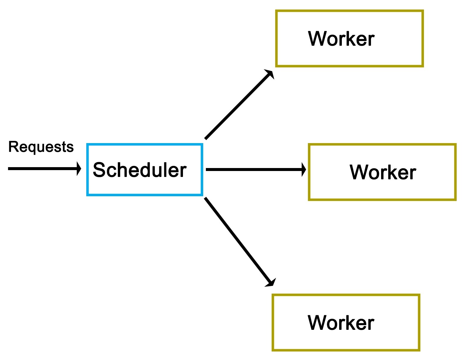
As one can see from the preceding high-level view, there really isn't much to it. However, as we'll see in a moment, the actual implementation does have a number of complications.
As is usual, we start off with the main function, contained in main.cpp:
#include "dispatcher.h"
#include "request.h"
#include <iostream>
#include <string>
#include <csignal>
#include <thread>
#include <chrono>
using namespace std;
sig_atomic_t signal_caught = 0;
mutex logMutex;
The custom headers we include are those for our dispatcher implementation, as well as the request class that we'll use.
Globally, we define an atomic variable to be used with the signal handler, as well as a mutex which will synchronize the output (on the standard output) from our logging method:
void sigint_handler(int sig) {
signal_caught = 1;
}
Our signal handler function (for SIGINT signals) simply sets the global atomic variable that we defined earlier:
void logFnc(string text) {
logMutex.lock();
cout << text << "n";
logMutex.unlock();
}
In our logging function, we use the global mutex to ensure that writing to the standard output is synchronized:
int main() {
signal(SIGINT, &sigint_handler);
Dispatcher::init(10);
In the main function, we install the signal handler for SIGINT to allow us to interrupt the execution of the application. We also call the static init() function on the Dispatcher class to initialize it:
cout << "Initialised.n";
int cycles = 0;
Request* rq = 0;
while (!signal_caught && cycles < 50) {
rq = new Request();
rq->setValue(cycles);
rq->setOutput(&logFnc);
Dispatcher::addRequest(rq);
cycles++;
}
Next, we set up the loop in which we will create new requests. In each cycle, we create a new Request instance, and use its setValue() function to set an integer value (current cycle number). We also set our logging function on the request instance before adding this new request to Dispatcher using its static addRequest() function.
This loop will continue until the maximum number of cycles have been reached, or SIGINT has been signaled using Ctrl+C or similar:
this_thread::sleep_for(chrono::seconds(5));
Dispatcher::stop();
cout << "Clean-up done.n";
return 0;
}
Finally, we wait for 5 seconds using the thread's sleep_for() function, and the chrono::seconds() function from the chrono STL header.
We also call the stop() function on Dispatcher before returning.
A request for Dispatcher always derives from the pure virtual AbstractRequest class:
#pragma once
#ifndef ABSTRACT_REQUEST_H
#define ABSTRACT_REQUEST_H
class AbstractRequest {
//
public:
virtual void setValue(int value) = 0;
virtual void process() = 0;
virtual void finish() = 0;
};
#endif
This AbstractRequest class defines an API with three functions, which a deriving class always has to implement. Out of these, the process() and finish() functions are the most generic and likely to be used in any practical implementation. The setValue() function is specific to this demonstration implementation, and would likely be adapted or extended to fit a real-life scenario.
The advantage of using an abstract class as the basis for a request is that it allows the Dispatcher class to handle many different types of requests as long as they all adhere to this same basic API.
Using this abstract interface, we implement a basic Request class as follows:
#pragma once
#ifndef REQUEST_H
#define REQUEST_H
#include "abstract_request.h"
#include <string>
using namespace std;
typedef void (*logFunction)(string text);
class Request : public AbstractRequest {
int value;
logFunction outFnc;
public: void setValue(int value) { this->value = value; }
void setOutput(logFunction fnc) { outFnc = fnc; }
void process();
void finish();
};
#endif
In its header file, we first define the function pointer's format. After this, we implement the request API, and add the setOutput() function to the base API, which accepts a function pointer for logging. Both setter functions merely assign the provided parameter to their respective private class members.
Next, the class function implementations are given as follows:
#include "request.h"
void Request::process() {
outFnc("Starting processing request " + std::to_string(value) + "...");
//
}
void Request::finish() {
outFnc("Finished request " + std::to_string(value));
}
Both of these implementations are very basic; they merely use the function pointer to output a string indicating the status of the worker thread.
In a practical implementation, one would add the business logic to the process() function with the finish() function containing any functionality to finish up a request such as writing a map into a string.
Next is the Worker class. This contains the logic which will be called by Dispatcher in order to process a request.
#pragma once
#ifndef WORKER_H
#define WORKER_H
#include "abstract_request.h"
#include <condition_variable>
#include <mutex>
using namespace std;
class Worker {
condition_variable cv;
mutex mtx;
unique_lock<mutex> ulock;
AbstractRequest* request;
bool running;
bool ready;
public:
Worker() { running = true; ready = false; ulock = unique_lock<mutex>(mtx); }
void run();
void stop() { running = false; }
void setRequest(AbstractRequest* request) { this->request = request; ready = true; }
void getCondition(condition_variable* &cv);
};
#endif
Whereas the adding of a request to Dispatcher does not require any special logic, the Worker class does require the use of condition variables to synchronize itself with the dispatcher. For the C++11 threads API, this requires a condition variable, a mutex, and a unique lock.
The unique lock encapsulates the mutex, and will ultimately be used with the condition variable as we will see in a moment.
Beyond this, we define methods to start and stop the worker, to set a new request for processing, and to obtain access to its internal condition variable.
Moving on, the rest of the implementation is written as follows:
#include "worker.h"
#include "dispatcher.h"
#include <chrono>
using namespace std;
void Worker::getCondition(condition_variable* &cv) {
cv = &(this)->cv;
}
void Worker::run() {
while (running) {
if (ready) {
ready = false;
request->process();
request->finish();
}
if (Dispatcher::addWorker(this)) {
// Use the ready loop to deal with spurious wake-ups.
while (!ready && running) {
if (cv.wait_for(ulock, chrono::seconds(1)) == cv_status::timeout) {
// We timed out, but we keep waiting unless
// the worker is
// stopped by the dispatcher.
}
}
}
}
}
Beyond the getter function for the condition variable, we define the run() function, which dispatcher will run for each worker thread upon starting it.
Its main loop merely checks that the stop() function hasn't been called yet, which would have set the running Boolean value to false, and ended the work thread. This is used by Dispatcher when shutting down, allowing it to terminate the worker threads. Since Boolean values are generally atomic, setting and checking can be done simultaneously without risk or requiring a mutex.
Moving on, the check of the ready variable is to ensure that a request is actually waiting when the thread is first run. On the first run of the worker thread, no request will be waiting, and thus, attempting to process one would result in a crash. Upon Dispatcher setting a new request, this Boolean variable will be set to true.
If a request is waiting, the ready variable will be set to false again, after which the request instance will have its process() and finish() functions called. This will run the business logic of the request on the worker thread's thread, and finalize it.
Finally, the worker thread adds itself to the dispatcher using its static addWorker() function. This function will return false if no new request is available, and cause the worker thread to wait until a new request has become available. Otherwise, the worker thread will continue with the processing of the new request that Dispatcher will have set on it.
If asked to wait, we enter a new loop. This loop will ensure that when the condition variable is woken up, it is because we got signaled by Dispatcher (ready variable set to true), and not because of a spurious wake-up.
Last of all, we enter the actual wait() function of the condition variable using the unique lock instance we created before along with a timeout. If a timeout occurs, we can either terminate the thread, or keep waiting. Here, we choose to do nothing and just re-enter the waiting loop.
As the last item, we have the Dispatcher class itself:
#pragma once
#ifndef DISPATCHER_H
#define DISPATCHER_H
#include "abstract_request.h"
#include "worker.h"
#include <queue>
#include <mutex>
#include <thread>
#include <vector>
using namespace std;
class Dispatcher {
static queue<AbstractRequest*> requests;
static queue<Worker*> workers;
static mutex requestsMutex;
static mutex workersMutex;
static vector<Worker*> allWorkers;
static vector<thread*> threads;
public:
static bool init(int workers);
static bool stop();
static void addRequest(AbstractRequest* request);
static bool addWorker(Worker* worker);
};
#endif
Most of this will look familiar. As you will have surmised by now, this is a fully static class.
Moving on, its implementation is as follows:
#include "dispatcher.h"
#include <iostream>
using namespace std;
queue<AbstractRequest*> Dispatcher::requests;
queue<Worker*> Dispatcher::workers;
mutex Dispatcher::requestsMutex;
mutex Dispatcher::workersMutex;
vector<Worker*> Dispatcher::allWorkers;
vector<thread*> Dispatcher::threads;
bool Dispatcher::init(int workers) {
thread* t = 0;
Worker* w = 0;
for (int i = 0; i < workers; ++i) {
w = new Worker;
allWorkers.push_back(w);
t = new thread(&Worker::run, w);
threads.push_back(t);
}
return true;
}
After setting up the static class members, the init() function is defined. It starts the specified number of worker threads keeping a reference to each worker and thread instance in their respective vector data structures:
bool Dispatcher::stop() {
for (int i = 0; i < allWorkers.size(); ++i) {
allWorkers[i]->stop();
}
cout << "Stopped workers.n";
for (int j = 0; j < threads.size(); ++j) {
threads[j]->join();
cout << "Joined threads.n";
}
}
In the stop() function, each worker instance has its stop() function called. This will cause each worker thread to terminate, as we saw earlier in the Worker class description.
Finally, we wait for each thread to join (that is, finish) prior to returning:
void Dispatcher::addRequest(AbstractRequest* request) {
workersMutex.lock();
if (!workers.empty()) {
Worker* worker = workers.front();
worker->setRequest(request);
condition_variable* cv;
worker->getCondition(cv);
cv->notify_one();
workers.pop();
workersMutex.unlock();
}
else {
workersMutex.unlock();
requestsMutex.lock();
requests.push(request);
requestsMutex.unlock();
}
}
The addRequest() function is where things get interesting. In this function, a new request is added. What happens next depends on whether a worker thread is waiting for a new request or not. If no worker thread is waiting (worker queue is empty), the request is added to the request queue.
The use of mutexes ensures that the access to these queues occurs safely, as the worker threads will simultaneously try to access both queues as well.
An important gotcha to note here is the possibility of a deadlock. That is, a situation where two threads will hold the lock on a resource, with the second thread waiting for the first one to release its lock before releasing its own. Every situation where more than one mutex is used in a single scope holds this potential.
In this function, the potential for a deadlock lies in releasing of the lock on the workers mutex, and when the lock on the requests mutex is obtained. In the case that this function holds the workers mutex and tries to obtain the requests lock (when no worker thread is available), there is a chance that another thread holds the requests mutex (looking for new requests to handle) while simultaneously trying to obtain the workers mutex (finding no requests and adding itself to the workers queue).
The solution here is simple: release a mutex before obtaining the next one. In the situation where one feels that more than one mutex lock has to be held, it is paramount to examine and test one's code for potential deadlocks. In this particular situation, the workers mutex lock is explicitly released when it is no longer needed, or before the requests mutex lock is obtained, thus preventing a deadlock.
Another important aspect of this particular section of code is the way it signals a worker thread. As one can see in the first section of the if/else block, when the workers queue is not empty, a worker is fetched from the queue, has the request set on it, and then has its condition variable referenced and signaled, or notified.
Internally, the condition variable uses the mutex we handed it before in the Worker class definition to guarantee only atomic access to it. When the notify_one() function (generally called signal() in other APIs) is called on the condition variable, it will notify the first thread in the queue of threads waiting for the condition variable to return and continue.
In the Worker class run() function, we would be waiting for this notification event. Upon receiving it, the worker thread would continue and process the new request. The thread reference will then be removed from the queue until it adds itself again once it is done processing the request:
bool Dispatcher::addWorker(Worker* worker) {
bool wait = true;
requestsMutex.lock();
if (!requests.empty()) {
AbstractRequest* request = requests.front();
worker->setRequest(request);
requests.pop();
wait = false;
requestsMutex.unlock();
}
else {
requestsMutex.unlock();
workersMutex.lock();
workers.push(worker);
workersMutex.unlock();
}
return wait;
}
With this last function, a worker thread will add itself to the queue once it is done processing a request. It is similar to the earlier function in that the incoming worker is first actively matched with any request which may be waiting in the request queue. If none are available, the worker is added to the worker queue.
It is important to note here that we return a Boolean value which indicates whether the calling thread should wait for a new request, or whether it already has received a new request while trying to add itself to the queue.
While this code is less complex than that of the previous function, it still holds the same potential deadlock issue due to the handling of two mutexes within the same scope. Here, too, we first release the mutex we hold before obtaining the next one.
The makefile for this Dispatcher example is very basic again--it gathers all C++ source files in the current folder, and compiles them into a binary using g++:
GCC := g++
OUTPUT := dispatcher_demo
SOURCES := $(wildcard *.cpp)
CCFLAGS := -std=c++11 -g3
all: $(OUTPUT)
$(OUTPUT):
$(GCC) -o $(OUTPUT) $(CCFLAGS) $(SOURCES)
clean:
rm $(OUTPUT)
.PHONY: all
After compiling the application, running it produces the following output for the 50 total requests:
$ ./dispatcher_demo.exe
Initialised.
Starting processing request 1...
Starting processing request 2...
Finished request 1
Starting processing request 3...
Finished request 3
Starting processing request 6...
Finished request 6
Starting processing request 8...
Finished request 8
Starting processing request 9...
Finished request 9
Finished request 2
Starting processing request 11...
Finished request 11
Starting processing request 12...
Finished request 12
Starting processing request 13...
Finished request 13
Starting processing request 14...
Finished request 14
Starting processing request 7...
Starting processing request 10...
Starting processing request 15...
Finished request 7
Finished request 15
Finished request 10
Starting processing request 16...
Finished request 16
Starting processing request 17...
Starting processing request 18...
Starting processing request 0...
At this point, we can already clearly see that even with each request taking almost no time to process, the requests are clearly being executed in parallel. The first request (request 0) only starts being processed after the sixteenth request, while the second request already finishes after the ninth request, long before this.
The factors which determine which thread, and thus, which request is processed first depends on the OS scheduler and hardware-based scheduling as described in chapter 9, Multithreading Implementation on the Processor and OS. This clearly shows just how few assumptions can be made about how a multithreaded application will be executed even on a single platform.
Starting processing request 5...
Finished request 5
Starting processing request 20...
Finished request 18
Finished request 20
Starting processing request 21...
Starting processing request 4...
Finished request 21
Finished request 4
In the preceding code, the fourth and fifth requests also finish in a rather delayed fashion.
Starting processing request 23...
Starting processing request 24...
Starting processing request 22...
Finished request 24
Finished request 23
Finished request 22
Starting processing request 26...
Starting processing request 25...
Starting processing request 28...
Finished request 26
Starting processing request 27...
Finished request 28
Finished request 27
Starting processing request 29...
Starting processing request 30...
Finished request 30
Finished request 29
Finished request 17
Finished request 25
Starting processing request 19...
Finished request 0
At this point, the first request finally finishes. This may indicate that the initialization time for the first request will always be delayed as compared to the successive requests. Running the application multiple times can confirm this. It's important that if the order of processing is relevant, this randomness does not negatively affect one's application.
Starting processing request 33...
Starting processing request 35...
Finished request 33
Finished request 35
Starting processing request 37...
Starting processing request 38...
Finished request 37
Finished request 38
Starting processing request 39...
Starting processing request 40...
Starting processing request 36...
Starting processing request 31...
Finished request 40
Finished request 39
Starting processing request 32...
Starting processing request 41...
Finished request 32
Finished request 41
Starting processing request 42...
Finished request 31
Starting processing request 44...
Finished request 36
Finished request 42
Starting processing request 45...
Finished request 44
Starting processing request 47...
Starting processing request 48...
Finished request 48
Starting processing request 43...
Finished request 47
Finished request 43
Finished request 19
Starting processing request 34...
Finished request 34
Starting processing request 46...
Starting processing request 49...
Finished request 46
Finished request 49
Finished request 45
Request 19 also became fairly delayed, showing once again just how unpredictable a multithreaded application can be. If we were processing a large dataset in parallel here, with chunks of data in each request, we might have to pause at some points to account for these delays, as otherwise, our output cache might grow too large.
As doing so would negatively affect an application's performance, one might have to look at low-level optimizations, as well as the scheduling of threads on specific processor cores in order to prevent this from happening.
Stopped workers.
Joined threads.
Joined threads.
Joined threads.
Joined threads.
Joined threads.
Joined threads.
Joined threads.
Joined threads.
Joined threads.
Joined threads.
Clean-up done.
All 10 worker threads which were launched in the beginning terminate here as we call the stop() function of the Dispatcher.
In the example given in this chapter, we saw how to share information between threads in addition to synchronizing threads--this in the form of the requests we passed from the main thread into the dispatcher from which each request gets passed on to a different thread.
The essential idea behind the sharing of data between threads is that the data to be shared exists somewhere in a way which is accessible to two threads or more. After this, we have to ensure that only one thread can modify the data, and that the data does not get modified while it's being read. Generally, we would use mutexes or similar to ensure this.
Read-write locks are a possible optimization here, because they allow multiple threads to read simultaneously from a single data source. If one has an application in which multiple worker threads read the same information repeatedly, it would be more efficient to use read-write locks than basic mutexes, because the attempts to read the data will not block the other threads.
A read-write lock can thus be used as a more advanced version of a mutex, namely, as one which adapts its behavior to the type of access. Internally, it builds on mutexes (or semaphores) and condition variables.
First available via the Boost library and introduced natively with C++11, shared pointers are an abstraction of memory management using reference counting for heap-allocated instances. They are partially thread-safe in that creating multiple shared pointer instances can be created, but the referenced object itself is not thread-safe.
Depending on the application, this may suffice, however. To make them properly thread-safe, one can use atomics. We will look at this in more detail in Chapter 15, Atomic Operations - Working with the Hardware.
In this chapter, we looked at how to pass data between threads in a safe manner as part of a fairly complex scheduler implementation. We also looked at the resulting asynchronous processing of the said scheduler, and considered some potential alternatives and optimizations for passing data between threads.
At this point, you should be able to safely pass data between threads, as well as synchronize access to other shared resources.
In the next chapter, we will look at native C++ threading and the primitives API.
Starting with the 2011 revision of the C++ standard, a multithreading API is officially part of the C++ Standard Template Library (STL). This means that threads, thread primitives, and synchronization mechanisms are available to any new C++ application without the need to install a third-party library, or to rely on the operating system's APIs.
This chapter looks at the multithreading features available in this native API up to the features added by the 2014 standard. A number of examples will be shown to use these features in detail.
Topics in this chapter include the following:
In Chapter 10, C++ Multithreading APIs, we looked at the various APIs that are available to us when developing a multithreaded C++ application. In Chapter 11, Thread Synchronization and Communication, we implemented a multithreaded scheduler application using the native C++ threading API.
By including the <thread> header from the STL, we gain access to the std::thread class with facilities for mutual exclusion (mutex, and so on) provided by further headers. This API is, essentially, the same as the multithreading API from Boost.Thread, the main differences being more control over threads (join with timeout, thread groups, and thread interruption), and a number of additional lock types implemented on top of primitives such as mutexes and condition variables.
In general, Boost.Thread should be used as a fall back for when C++11 support isn't present, or when these additional Boost.Thread features are a requirement of one's application, and not easily added otherwise. Since Boost.Thread builds upon the available (native) threading support, it's also likely to add overhead as compared to the C++11 STL implementation.
The 2011 revision to the C++ standard (commonly referred to as C++11) adds a wide range of new features, the most crucial one being the addition of native multithreading support, which adds the ability to create, manage, and use threads within C++ without the use of third-party libraries.
This standard standardizes the memory model for the core language to allow multiple threads to coexist as well as enables features such as thread-local storage. Initial support was added in the C++03 standard, but the C++11 standard is the first to make full use of this.
As noted earlier, the actual threading API itself is implemented in the STL. One of the goals for the C++11 (C++0x) standard was to have as many of the new features as possible in the STL, and not as part of the core language. As a result, in order to use threads, mutexes, and kin, one has to first include the relevant STL header.
The standards committee which worked on the new multithreading API each had their own sets of goals, and as a result, a few features which were desired by some did not make it into the final standard. This includes features such as terminating another thread, or thread cancellation, which was strongly opposed by the POSIX representatives on account of canceling threads likely to cause issues with resource clean-up in the thread being destroyed.
Following are the features provided by this API implementation:
In a moment, we will look at detailed examples of each of these features. First we will see what the next revisions of the C++ standard have added to this initial set.
The 2014 standard adds the following features to the standard library:
Both of these are defined in the <shared_mutex> STL header. Since locks are based on mutexes, a shared lock is, therefore, reliant on a shared mutex.
The thread class is the core of the entire threading API; it wraps the underlying operating system's threads, and provides the functionality we need to start and stop threads.
This functionality is made accessible by including the <thread> header.
Upon creating a thread it is started immediately:
#include <thread>
void worker() {
// Business logic.
}
int main () {
std::thread t(worker);
return 0;
}
This preceding code would start the thread to then immediately terminate the application, because we are not waiting for the new thread to finish executing.
To do this properly, we need to wait for the thread to finish, or rejoin as follows:
#include <thread>
void worker() {
// Business logic.
}
int main () {
std::thread t(worker);
t.join();
return 0;
}
This last code would execute, wait for the new thread to finish, and then return.
It's also possible to pass parameters to a new thread. These parameter values have to be move constructible, which means that it's a type which has a move or copy constructor (called for rvalue references). In practice, this is the case for all basic types and most (user-defined) classes:
#include <thread>
#include <string>
void worker(int n, std::string t) {
// Business logic.
}
int main () {
std::string s = "Test";
int i = 1;
std::thread t(worker, i, s);
t.join();
return 0;
}
In this preceding code, we pass an integer and string to the thread function. This function will receive copies of both variables. When passing references or pointers, things get more complicated with life cycle issues, data races, and such becoming a potential problem.
Any value returned by the function passed to the thread class constructor is ignored. To return information to the thread which created the new thread, one has to use inter-thread synchronization mechanisms (like mutexes) and some kind of a shared variable.
The 2011 standard adds std::move to the <utility> header. Using this template method, one can move resources between objects. This means that it can also move thread instances:
#include <thread>
#include <string>
#include <utility>
void worker(int n, string t) {
// Business logic.
}
int main () {
std::string s = "Test";
std::thread t0(worker, 1, s);
std::thread t1(std::move(t0));
t1.join();
return 0;
}
In this version of the code, we create a thread before moving it to another thread. Thread 0 thus ceases to exist (since it instantly finishes), and the execution of the thread function resumes in the new thread that we create.
As a result of this, we do not have to wait for the first thread to re join, but only for the second one.
Each thread has an identifier associated with it. This ID, or handle, is a unique identifier provided by the STL implementation. It can be obtained by calling the get_id() function of the thread class instance, or by calling std::this_thread::get_id() to get the ID of the thread calling the function:
#include <iostream>
#include <thread>
#include <chrono>
#include <mutex>
std::mutex display_mutex;
void worker() {
std::thread::id this_id = std::this_thread::get_id();
display_mutex.lock();
std::cout << "thread " << this_id << " sleeping...n";
display_mutex.unlock();
std::this_thread::sleep_for(std::chrono::seconds(1));
}
int main() {
std::thread t1(worker);
std::thread::id t1_id = t1.get_id();
std::thread t2(worker);
std::thread::id t2_id = t2.get_id();
display_mutex.lock();
std::cout << "t1's id: " << t1_id << "n";
std::cout << "t2's id: " << t2_id << "n";
display_mutex.unlock();
t1.join();
t2.join();
return 0;
}
This code would produce output similar to this:
t1's id: 2
t2's id: 3
thread 2 sleeping...
thread 3 sleeping...
Here, one sees that the internal thread ID is an integer (std::thread::id type), relative to the initial thread (ID 1). This is comparable to most native thread IDs such as those for POSIX. These can also be obtained using native_handle(). That function will return whatever is the underlying native thread handle. It is particularly useful when one wishes to use a very specific PThread or Win32 thread functionality that's not available in the STL implementation.
It's possible to delay the execution of a thread (sleep) using either of two methods. One is sleep_for(), which delays execution by at least the specified duration, but possibly longer:
#include <iostream>
#include <chrono>
#include <thread>
using namespace std::chrono_literals;
typedef std::chrono::time_point<std::chrono::high_resolution_clock> timepoint;
int main() {
std::cout << "Starting sleep.n";
timepoint start = std::chrono::high_resolution_clock::now();
std::this_thread::sleep_for(2s);
timepoint end = std::chrono::high_resolution_clock::now();
std::chrono::duration<double, std::milli> elapsed = end -
start;
std::cout << "Slept for: " << elapsed.count() << " msn";
}
This preceding code shows how to sleep for roughly 2 seconds, measuring the exact duration using a counter with the highest precision possible on the current OS.
Note that we are able to specify the number of seconds directly, with the seconds post-fix. This is a C++14 feature that got added to the <chrono> header. For the C++11 version, one has to create an instance of std::chrono::seconds and pass it to the sleep_for() function.
The other method is sleep_until(), which takes a single parameter of type std::chrono::time_point<Clock, Duration>. Using this function, one can set a thread to sleep until the specified time point has been reached. Due to the operating system's scheduling priorities, this wake-up time might not be the exact time as specified.
One can indicate to the OS that the current thread can be rescheduled so that other threads can run instead. For this, one uses the std::this_thread::yield() function. The exact result of this function depends on the underlying OS implementation and its scheduler. In the case of a FIFO scheduler, it's likely that the calling thread will be put at the back of the queue.
This is a highly specialized function, with special use cases. It should not be used without first validating its effect on the application's performance.
After starting a thread, one can call detach() on the thread object. This effectively detaches the new thread from the calling thread, meaning that the former will continue executing even after the calling thread has exited.
Using swap(), either as a standalone method or as function of a thread instance, one can exchange the underlying thread handles of thread objects:
#include <iostream>
#include <thread>
#include <chrono>
void worker() {
std::this_thread::sleep_for(std::chrono::seconds(1));
}
int main() {
std::thread t1(worker);
std::thread t2(worker);
std::cout << "thread 1 id: " << t1.get_id() << "n";
std::cout << "thread 2 id: " << t2.get_id() << "n";
std::swap(t1, t2);
std::cout << "Swapping threads..." << "n";
std::cout << "thread 1 id: " << t1.get_id() << "n";
std::cout << "thread 2 id: " << t2.get_id() << "n";
t1.swap(t2);
std::cout << "Swapping threads..." << "n";
std::cout << "thread 1 id: " << t1.get_id() << "n";
std::cout << "thread 2 id: " << t2.get_id() << "n";
t1.join();
t2.join();
}
The possible output from this code might look like the following:
thread 1 id: 2
thread 2 id: 3
Swapping threads...
thread 1 id: 3
thread 2 id: 2
Swapping threads...
thread 1 id: 2
thread 2 id: 3
The effect of this is that the state of each thread is swapped with that of the other thread, essentially exchanging their identities.
The <mutex> header contains multiple types of mutexes and locks. The mutex type is the most commonly used type, and provides the basic lock/unlock functionality without any further complications.
At its core, the goal of a mutex is to exclude the possibility of simultaneous access so as to prevent data corruption, and to prevent crashes due to the use of non-thread-safe routines.
An example of where one would need to use a mutex is the following code:
#include <iostream>
#include <thread>
void worker(int i) {
std::cout << "Outputting this from thread number: " << i << "n";
}
int main() {
std::thread t1(worker, 1);
std::thread t2(worker, 2);
t1.join();
t2.join();
return 0;
}
If one were to try and run this preceding code as-is, one would notice that the text output from both threads would be mashed together instead of being output one after the other. The reason for this is that the standard output (whether C or C++-style) is not thread-safe. Though the application will not crash, the output will be a jumble.
The fix for this is simple, and is given as follows:
#include <iostream>
#include <thread>
#include <mutex>
std::mutex globalMutex;
void worker(int i) {
globalMutex.lock();
std::cout << "Outputting this from thread number: " << i << "n";
globalMutex.unlock();
}
int main() {
std::thread t1(worker, 1);
std::thread t2(worker, 2);
t1.join();
t2.join();
return 0;
}
In this situation, each thread would first need to obtain access to the mutex object. Since only one thread can have access to the mutex object, the other thread will end up waiting for the first thread to finish writing to the standard output, and the two strings will appear one after the other, as intended.
It's possible to not want the thread to block and wait for the mutex object to become available: for example, when one just wants to know whether a request is already being handled by another thread, and there's no use in waiting for it to finish.
For this, a mutex comes with the try_lock() function which does exactly that.
In the following example, we can see two threads trying to increment the same counter, but with one incrementing its own counter whenever it fails to immediately obtain access to the shared counter:
#include <chrono>
#include <mutex>
#include <thread>
#include <iostream>
std::chrono::milliseconds interval(50);
std::mutex mutex;
int shared_counter = 0;
int exclusive_counter = 0;
void worker0() {
std::this_thread::sleep_for(interval);
while (true) {
if (mutex.try_lock()) {
std::cout << "Shared (" << job_shared << ")n";
mutex.unlock();
return;
}
else {
++exclusive_counter;
std::cout << "Exclusive (" << exclusive_counter << ")n";
std::this_thread::sleep_for(interval);
}
}
}
void worker1() {
mutex.lock();
std::this_thread::sleep_for(10 * interval);
++shared_counter;
mutex.unlock();
}
int main() {
std::thread t1(worker0);
std::thread t2(worker1);
t1.join();
t2.join();
}
Both threads in this preceding example run a different worker function, yet both have in common the fact that they sleep for a period of time, and try to acquire the mutex for the shared counter when they wake up. If they do, they'll increase the counter, but only the first worker will output this fact.
The first worker also logs when it did not get the shared counter, but only increased its exclusive counter. The resulting output might look something like this:
Exclusive (1)
Exclusive (2)
Exclusive (3)
Shared (1)
Exclusive (4)
A timed mutex is a regular mutex type, but with a number of added functions which give one control over the time period during which it should be attempted to obtain the lock, that is, try_lock_for and try_lock_until.
The former tries to obtain the lock during the specified time period (std::chrono object) before returning the result (true or false). The latter will wait until a specific point in the future before returning the result.
The use of these functions mostly lies in offering a middle path between the blocking (lock) and non-blocking (try_lock) methods of the regular mutex. One may want to wait for a number of tasks using only a single thread without knowing when a task will become available, or a task may expire at a certain point in time at which waiting for it makes no sense any more.
A lock guard is a simple mutex wrapper, which handles the obtaining of a lock on the mutex object as well as its release when the lock guard goes out of scope. This is a helpful mechanism to ensure that one does not forget to release a mutex lock, and to help reduce clutter in one's code when one has to release the same mutex in multiple locations.
While refactoring of, for example, big if/else blocks can reduce the instances in which the release of a mutex lock is required, it's much easier to just use this lock guard wrapper and not worry about such details:
#include <thread>
#include <mutex>
#include <iostream>
int counter = 0;
std::mutex counter_mutex;
void worker() {
std::lock_guard<std::mutex> lock(counter_mutex);
if (counter == 1) { counter += 10; }
else if (counter >= 10) { counter += 15; }
else if (counter >= 50) { return; }
else { ++counter; }
std::cout << std::this_thread::get_id() << ": " << counter << 'n';
}
int main() {
std::cout << __func__ << ": " << counter << 'n';
std::thread t1(worker);
std::thread t2(worker);
t1.join();
t2.join();
std::cout << __func__ << ": " << counter << 'n';
}
In the preceding example, we see that we have a small if/else block with one condition leading to the worker function immediately returning. Without a lock guard, we would have to make sure that we also unlocked the mutex in this condition before returning from the function.
With the lock guard, however, we do not have to worry about such details, which allows us to focus on the business logic instead of worrying about mutex management.
The unique lock is a general-purpose mutex wrapper. It's similar to the timed mutex, but with additional features, primary of which is the concept of ownership. Unlike other lock types, a unique lock does not necessarily own the mutex it wraps if it contains any at all. Mutexes can be transferred between unique lock instances along with ownership of the said mutexes using the swap() function.
Whether a unique lock instance has ownership of its mutex, and whether it's locked or not, is first determined when creating the lock, as can be seen with its constructors. For example:
std::mutex m1, m2, m3;
std::unique_lock<std::mutex> lock1(m1, std::defer_lock);
std::unique_lock<std::mutex> lock2(m2, std::try_lock);
std::unique_lock<std::mutex> lock3(m3, std::adopt_lock);
The first constructor in the last code does not lock the assigned mutex (defers). The second attempts to lock the mutex using try_lock(). Finally, the third constructor assumes that it already owns the provided mutex.
In addition to these, other constructors allow the functionality of a timed mutex. That is, it will wait for a time period until a time point has been reached, or until the lock has been acquired.
Finally, the association between the lock and the mutex is broken by using the release() function, and a pointer is returned to the mutex object. The caller is then responsible for the releasing of any remaining locks on the mutex and for the further handling of it.
This type of lock isn't one which one will tend to use very often on its own, as it's extremely generic. Most of the other types of mutexes and locks are significantly less complex, and likely to fulfil all the needs in 99% of all cases. The complexity of a unique lock is, thus, both a benefit and a risk.
It is, however, commonly used by other parts of the C++11 threading API, such as condition variables, as we will see in a moment.
One area where a unique lock may be useful is as a scoped lock, allowing one to use scoped locks without having to rely on the native scoped locks in the C++17 standard. See this example:
#include <mutex>
std::mutex my_mutex
int count = 0;
int function() {
std::unique_lock<mutex> lock(my_mutex);
count++;
}
As we enter the function, we create a new unique_lock with the global mutex instance. The mutex is locked at this point, after which we can perform any critical operations.
When the function scope ends, the destructor of the unique_lock is called, which results in the mutex getting unlocked again.
First introduced in the 2017 standard, the scoped lock is a mutex wrapper which obtains access to (locks) the provided mutex, and ensures it is unlocked when the scoped lock goes out of scope. It differs from a lock guard in that it is a wrapper for not one, but multiple mutexes.
This can be useful when one deals with multiple mutexes in a single scope. One reason to use a scoped lock is to avoid accidentally introducing deadlocks and other unpleasant complications with, for example, one mutex being locked by the scoped lock, another lock still being waited upon, and another thread instance having the exactly opposite situation.
One property of a scoped lock is that it tries to avoid such a situation, theoretically making this type of lock deadlock-safe.
The recursive mutex is another subtype of mutex. Even though it has exactly the same functions as a regular mutex, it allows the calling thread, which initially locked the mutex, to lock the same mutex repeatedly. By doing this, the mutex doesn't become available for other threads until the owning thread has unlocked the mutex as many times as it has locked it.
One good reason to use a recursive mutex is for example when using recursive functions. With a regular mutex one would need to invent some kind of entry point which would lock the mutex before entering the recursive function.
With a recursive mutex, each iteration of the recursive function would lock the recursive mutex again, and upon finishing one iteration, it would unlock the mutex. As a result the mutex would be unlocked and unlocked the same number of times.
A potential complication hereby is that the maximum number of times that a recursive mutex can be locked is not defined in the standard. When the implementation's limit has been reached, a std::system_error will be thrown if one tries to lock it, or false is returned when using the non-blocking try_lock function.
The recursive timed mutex is, as the name suggests, an amalgamation of the functionality of the timed mutex and recursive mutex. As a result, it allows one to recursively lock the mutex using a timed conditional function.
Although this adds challenges to ensuring that the mutex is unlocked as many times as the thread locks it, it nevertheless offers possibilities for more complex algorithms such as the aforementioned task-handlers.
The <shared_mutex> header was first added with the 2014 standard, by adding the shared_timed_mutex class. With the 2017 standard, the shared_mutex class was also added.
The shared mutex header has been present since C++17. In addition to the usual mutual exclusive access, this mutex class adds the ability to provide shared access to the mutex. This allows one to, for example, provide read access to a resource by multiple threads, while a writing thread would still be able to gain exclusive access. This is similar to the read-write locks of Pthreads.
The functions added to this mutex type are the following:
The use of this mutex's share functionality should be fairly self-explanatory. A theoretically infinite number of readers can gain read access to the mutex, while ensuring that only a single thread can write to the resource at any time.
This header has been present since C++14. It adds shared locking functionality to the timed mutex with these functions:
This class is essentially an amalgamation of the shared mutex and timed mutex, as the name suggests. The interesting thing here is that it was added to the standard before the more basic shared mutex.
In essence, a condition variable provides a mechanism through which a thread's execution can be controlled by another thread. This is done by having a shared variable which a thread will wait for until signaled by another thread. It is an essential part of the scheduler implementation we looked at in Chapter 11, Thread Synchronization and Communication.
For the C++11 API, condition variables and their associated functionality are defined in the <condition_variable> header.
The basic usage of a condition variable can be summarized from that scheduler's code in Chapter 11, Thread Synchronization and Communication.
#include "abstract_request.h"
#include <condition_variable>
#include <mutex>
using namespace std;
class Worker {
condition_variable cv;
mutex mtx;
unique_lock<mutex> ulock;
AbstractRequest* request;
bool running;
bool ready;
public:
Worker() { running = true; ready = false; ulock = unique_lock<mutex>(mtx); }
void run();
void stop() { running = false; }
void setRequest(AbstractRequest* request) { this->request = request; ready = true; }
void getCondition(condition_variable* &cv);
};
In the constructor, as defined in the preceding Worker class declaration, we see the way a condition variable in the C++11 API is initialized. The steps are listed as follows:
#include <chrono>
using namespace std;
void Worker::run() {
while (running) {
if (ready) {
ready = false;
request->process();
request->finish();
}
if (Dispatcher::addWorker(this)) {
while (!ready && running) {
if (cv.wait_for(ulock, chrono::seconds(1)) ==
cv_status::timeout) {
// We timed out, but we keep waiting unless the
worker is
// stopped by the dispatcher.
}
}
}
}
}
Here, we use the wait_for() function of the condition variable, and pass both the unique lock instance we created earlier and the amount of time which we want to wait for. Here we wait for 1 second. If we time out on this wait, we are free to re-enter the wait (as is done here) in a continuous loop, or continue execution.
It's also possible to perform a blocking wait using the simple wait() function, or wait until a certain point in time with wait_for().
As noted, when we first looked at this code, the reason why this worker's code uses the ready Boolean variable is to check that it was really another thread which signaled the condition variable, and not just a spurious wake-up. It's an unfortunate complication of most condition variable implementations--including the C++11 one--that they are susceptible to this.
As a result of these random wake-up events, it is necessary to have some way to ensure that we really did wake up intentionally. In the scheduler code, this is done by having the thread which wakes up the worker thread also set a Boolean value which the worker thread can wake up.
Whether we timed out, or were notified, or suffered a spurious wake-up can be checked with the cv_status enumeration. This enumeration knows these two possible conditions:
The signaling, or notifying, itself is quite straightforward:
void Dispatcher::addRequest(AbstractRequest* request) {
workersMutex.lock();
if (!workers.empty()) {
Worker* worker = workers.front();
worker->setRequest(request);
condition_variable* cv;
worker->getCondition(cv);
cv->notify_one();
workers.pop();
workersMutex.unlock();
}
else {
workersMutex.unlock();
requestsMutex.lock();
requests.push(request);
requestsMutex.unlock();
}
}
In this preceding function from the Dispatcher class, we attempt to obtain an available worker thread instance. If found, we obtain a reference to the worker thread's condition variable as follows:
void Worker::getCondition(condition_variable* &cv) {
cv = &(this)->cv;
}
Setting the new request on the worker thread also changes the value of the ready variable to true, allowing the worker to check that it is indeed allowed to continue.
Finally, the condition variable is notified that any threads which are waiting on it can now continue using notify_one(). This particular function will signal the first thread in the FIFO queue for this condition variable to continue. Here, only one thread will ever be notified, but if there are multiple threads waiting for the same condition variable, the calling of notify_all() will allow all threads in the FIFO queue to continue.
The condition_variable_any class is a generalization of the condition_variable class. It differs from the latter in that it allows for other mutual exclusion mechanisms to be used beyond unique_lock<mutex>. The only requirement is that the lock used meets the BasicLockable requirements, meaning that it provides a lock() and unlock() function.
The std::notify_all_at_thread_exit() function allows a (detached) thread to notify other threads that it has completely finished, and is in the process of having all objects within its scope (thread-local) destroyed. It functions by moving the provided lock to internal storage before signaling the provided condition variable.
The result is exactly as if the lock was unlocked and notify_all() was called on the condition variable.
A basic (non-functional) example can be given as follows:
#include <mutex>
#include <thread>
#include <condition_variable>
using namespace std;
mutex m;
condition_variable cv;
bool ready = false;
ThreadLocal result;
void worker() {
unique_lock<mutex> ulock(m);
result = thread_local_method();
ready = true;
std::notify_all_at_thread_exit(cv, std::move(ulock));
}
int main() {
thread t(worker);
t.detach();
// Do work here.
unique_lock<std::mutex> ulock(m);
while(!ready) {
cv.wait(ulock);
}
// Process result
}
Here, the worker thread executes a method which creates thread-local objects. It's therefore essential that the main thread waits for the detached worker thread to finish first. If the latter isn't done yet when the main thread finishes its tasks, it will enter a wait using the global condition variable. In the worker thread, std::notify_all_at_thread_exit() is called after setting the ready Boolean.
What this accomplishes is twofold. After calling the function, no more threads are allowed to wait on the condition variable. It also allows the main thread to wait for the result of the detached worker thread to become available.
The last part of the C++11 thread support API is defined in <future>. It offers a range of classes, which implement more high-level multithreading concepts aimed more at easy asynchronous processing rather than the implementation of a multithreaded architecture.
Here we have to distinguish two concepts: that of a future and that of a promise. The former is the end result (the future product) that'll be used by a reader/consumer. The latter is what the writer/producer uses.
A basic example of a future would be:
#include <iostream>
#include <future>
#include <chrono>
bool is_prime (int x) {
for (int i = 2; i < x; ++i) if (x%i==0) return false;
return true;
}
int main () {
std::future<bool> fut = std::async (is_prime, 444444443);
std::cout << "Checking, please wait";
std::chrono::milliseconds span(100);
while (fut.wait_for(span) == std::future_status::timeout) { std::cout << '.' << std::flush;
}
bool x = fut.get();
std::cout << "n444444443 " << (x?"is":"is not") << " prime.n";
return 0;
}
This code asynchronously calls a function, passing it a parameter (potential prime number). It then enters an active loop while it waits for the future it received from the asynchronous function call to finish. It sets a 100 ms timeout on its wait function.
Once the future finishes (not returning a timeout on the wait function), we obtain the resulting value, in this case telling us that the value we provided the function with is in fact a prime number.
In the async section of this chapter, we will look a bit more at asynchronous function calls.
A promise allows one to transfer states between threads. For example:
#include <iostream>
#include <functional>
#include <thread>
#include <future>
void print_int (std::future<int>& fut) {
int x = fut.get();
std::cout << "value: " << x << 'n';
}
int main () {
std::promise<int> prom;
std::future<int> fut = prom.get_future();
std::thread th1 (print_int, std::ref(fut));
prom.set_value (10);
th1.join();
return 0;
This preceding code uses a promise instance passed to a worker thread to transfer a value to the other thread, in this case an integer. The new thread waits for the future we created from the promise, and which it received from the main thread to complete.
The promise is completed when we set the value on the promise. This completes the future and finishes the worker thread.
In this particular example, we use a blocking wait on the future object, but one can also use wait_for() and wait_until(), to wait for a time period or a point in time respectively, as we saw in the previous example for a future.
A shared_future is just like a regular future object, but can be copied, which allows multiple threads to read its results.
Creating a shared_future is similar to a regular future.
std::promise<void> promise1;
std::shared_future<void> sFuture(promise1.get_future());
The biggest difference is that the regular future is passed to its constructor.
After this, all threads which have access to the future object can wait for it, and obtain its value. This can also be used to signal threads in a way similar to condition variables.
A packaged_task is a wrapper for any callable target (function, bind, lambda, or other function object). It allows for asynchronous execution with the result available in a future object. It is similar to std::function, but automatically transfers its results to a future object.
For example:
#include <iostream>
#include <future>
#include <chrono>
#include <thread>
using namespace std;
int countdown (int from, int to) {
for (int i = from; i != to; --i) {
cout << i << 'n';
this_thread::sleep_for(chrono::seconds(1));
}
cout << "Finished countdown.n";
return from - to;
}
int main () {
packaged_task<int(int, int)> task(countdown);
future<int> result = task.get_future();
thread t (std::move(task), 10, 0);
// Other logic.
int value = result.get();
cout << "The countdown lasted for " << value << " seconds.n";
t.join();
return 0;
}
This preceding code implements a simple countdown feature, counting down from 10 to 0. After creating the task and obtaining a reference to its future object, we push it onto a thread along with the parameters of the worker function.
The result from the countdown worker thread becomes available as soon as it finishes. We can use the future object's waiting functions here the same way as for a promise.
A more straightforward version of promise and packaged_task can be found in std::async(). This is a simple function, which takes a callable object (function, bind, lambda, and similar) along with any parameters for it, and returns a future object.
The following is a basic example of the async() function:
#include <iostream>
#include <future>
using namespace std;
bool is_prime (int x) {
cout << "Calculating prime...n";
for (int i = 2; i < x; ++i) {
if (x % i == 0) {
return false;
}
}
return true;
}
int main () {
future<bool> pFuture = std::async (is_prime, 343321);
cout << "Checking whether 343321 is a prime number.n";
// Wait for future object to be ready.
bool result = pFuture.get();
if (result) {
cout << "Prime found.n";
}
else {
cout << "No prime found.n";
}
return 0;
}
The worker function in the preceding code determines whether a provided integer is a prime number or not. As we can see, the resulting code is a lot more simple than with a packaged_task or promise.
In addition to the basic version of std::async(), there is a second version which allows one to specify the launch policy as its first argument. This is a bitmask value of type std::launch with the following possible values:
* launch::async
* launch::deferred
The async flag means that a new thread and execution context for the worker function is created immediately. The deferred flag means that this is postponed until wait() or get() is called on the future object. Specifying both flags causes the function to choose the method automatically depending on the current system situation.
The std::async() version, without explicitly specified bitmask values, defaults to the latter, automatic method.
With multithreading, the use of atomics is also very important. The C++11 STL offers an <atomic> header for this reason. This topic is covered extensively in Chapter 15, Atomic Operations - Working with the Hardware.
In this chapter, we explored the entirety of the multithreading support in the C++11 API, along with the features added in C++14 and C++17.
We saw how to use each feature using descriptions and example code. We can now use the native C++ multithreading API to implement multithreaded, thread-safe code as well as use the asynchronous execution features in order to speed up and execute functions in parallel.
In the next chapter, we will take a look at the inevitable next step in the implementation of multithreaded code: debugging and validating of the resulting application.
Ideally, one's code would work properly the first time around, and contain no hidden bugs that are waiting to crash the application, corrupt data, or cause other issues. Realistically, this is, of course, impossible. Thus it is that tools were developed which make it easy to examine and debug multithreaded applications.
In this chapter, we will look at a number of them including a regular debugger as well as some of the tools which are part of the Valgrind suite, specifically, Helgrind and DRD. We will also look at profiling a multithreaded application in order to find hotspots and potential issues in its design.
Topics covered in this chapter include the following:
Ideally, one would test and validate one's code every time one has reached a certain milestone, whether it's for a singular module, a number of modules, or the application as a whole. It's important to ascertain that the assumptions one makes match up with the ultimate functionality.
Especially, with multithreaded code, there's a large element of coincidence in that a particular error state is not guaranteed to be reached during each run of the application. Signs of an improperly implemented multithreaded application may result in symptoms such as seemingly random crashes.
Likely the first hint one will get that something isn't correct is when the application crashes, and one is left with a core dump. This is a file which contains the memory content of the application at the time when it crashed, including the stack.
This core dump can be used in almost the same fashion as running a debugger with the running process. It is particularly useful to examine the location in the code at which we crashed, and in which thread. We can also examine memory contents this way.
One of the best indicators that one is dealing with a multithreading issue is when the application never crashes in the same location (different stack trace), or when it always crashes around a point where one performs mutual exclusion operations, such as manipulating a global data structure.
To start off, we'll first take a more in-depth look at using a debugger for diagnosing and debugging before diving into the Valgrind suite of tools.
Of all the questions a developer may have, the question of why did my application just crash? is probably among the most important. This is also one of the questions which are most easily answered with a debugger. Regardless of whether one is live debugging a process, or analyzing the core dump of a crashed process, the debugger can (hopefully) generate a back trace, also known as a stack trace. This trace contains a chronological list of all the functions which were called since the application was started as one would find them on the stack (see chapter 9, Multithreading Implementation on the Processor and OS, for details on how a stack works).
The last few entries of this back trace will thus show us in which part of the code things went wrong. If the debug information was compiled into the binary, or provided to the debugger, we can also see the code at that line along with the names of the variables.
Even better, since we're looking at the stack frames, we can also examine the variables within that stack frame. This means the parameters passed to the function along with any local variables and their values.
In order to have the debug information (symbols) available, one has to compile the source code with the appropriate compiler flags set. For GCC, one can select a host of debug information levels and types. Most commonly, one would use the -g flag with an integer specifying the debug level attached, as follows:
This flag instructs GCC to generate debug information in the native format for the OS. One can also use different flags to generate the debug information in a specific format; however, this is not necessary for use with GCC's debugger (GDB) as well as with the Valgrind tools.
Both GDB and Valgrind will use this debug information. While it's technically possible to use both without having the debug information available, that's best left as an exercise for truly desperate times.
One of the most commonly used debuggers for C-based and C++-based code is the GNU Debugger, or GDB for short. In the following example, we'll use this debugger due to it being both widely used and freely available. Originally written in 1986, it's now used with a wide variety of programming languages, and has become the most commonly used debugger, both in personal and professional use.
The most elemental interface for GDB is a command-line shell, but it can be used with graphical frontends, which also include a number of IDEs such as Qt Creator, Dev-C++, and Code::Blocks. These frontends and IDEs can make it easier and more intuitive to manage breakpoints, set up watch variables, and perform other common operations. Their use is, however, not required.
On Linux and BSD distributions, gdb is easily installed from a package, just as it is on Windows with MSYS2 and similar UNIX-like environments. For OS X/MacOS, one may have to install gdb using a third-party package manager such as Homebrew.
Since gdb is not normally code signed on MacOS, it cannot gain the system-level access it requires for normal operation. Here one can either run gdb as root (not recommended), or follow a tutorial relevant to your version of MacOS.
As mentioned earlier, there are two ways to use a debugger, either by starting the application from within the debugger (or attaching to the running process), or by loading a core dump file. Within the debugging session, one can either interrupt the running process (with Ctrl+C, which sends the SIGINT signal), or load the debug symbols for the loaded core dump. After this, we can examine the active threads in this frame:
Thread 1 received signal SIGINT, Interrupt.
0x00007fff8a3fff72 in mach_msg_trap () from /usr/lib/system/libsystem_kernel.dylib
(gdb) info threads
Id Target Id Frame
* 1 Thread 0x1703 of process 72492 0x00007fff8a3fff72 in mach_msg_trap () from /usr/lib/system/libsystem_kernel.dylib
3 Thread 0x1a03 of process 72492 0x00007fff8a406efa in kevent_qos () from /usr/lib/system/libsystem_kernel.dylib
10 Thread 0x2063 of process 72492 0x00007fff8a3fff72 in mach_msg_trap () from /usr/lib/system/libsystem_kernel.dylibs
14 Thread 0x1e0f of process 72492 0x00007fff8a405d3e in __pselect () from /usr/lib/system/libsystem_kernel.dylib
(gdb) c
Continuing.
In the preceding code, we can see how after sending the SIGINT signal to the application (a Qt-based application running on OS X), we request the list of all threads which exist at this point in time along with their thread number, ID, and the function which they are currently executing. This also shows clearly which threads are likely waiting based on the latter information, as is often the case of a graphical user interface application like this one. Here we also see that the thread which is currently active in the application as marked by the asterisk in front of its number (thread 1).
We can also switch between threads at will by using the thread <ID> command, and move up and down between a thread's stack frames. This allows us to examine every aspect of individual threads.
When full debug information is available, one would generally also see the exact line of code that a thread is executing. This means that during the development stage of an application, it makes sense to have as much debug information available as possible to make debugging much easier.
For the dispatcher code we looked at in Chapter 11, Threading Synchronization and Communication, we can set a breakpoint to allow us to examine the active threads as well:
$ gdb dispatcher_demo.exe
GNU gdb (GDB) 7.9
Copyright (C) 2015 Free Software Foundation, Inc.
Reading symbols from dispatcher_demo.exe...done.
(gdb) break main.cpp:67
Breakpoint 1 at 0x4017af: file main.cpp, line 67.
(gdb) run
Starting program: dispatcher_demo.exe
[New Thread 10264.0x2a90]
[New Thread 10264.0x2bac]
[New Thread 10264.0x2914]
[New Thread 10264.0x1b80]
[New Thread 10264.0x213c]
[New Thread 10264.0x2228]
[New Thread 10264.0x2338]
[New Thread 10264.0x270c]
[New Thread 10264.0x14ac]
[New Thread 10264.0x24f8]
[New Thread 10264.0x1a90]
As we can see in the above command line output, we start GDB with the name of the application we wish to debug as a parameter, here from a Bash shell under Windows. After this, we can set a breakpoint here, using the filename of the source file and the line we wish to break at after the (gdb) of the gdb command line input. We select the first line after the loop in which the requests get sent to the dispatcher, then run the application. This is followed by the list of the new threads which are being created by the dispatcher, as reported by GDB.
Next, we wait until the breakpoint is hit:
Breakpoint 1, main () at main.cpp:67
67 this_thread::sleep_for(chrono::seconds(5));
(gdb) info threads
Id Target Id Frame
11 Thread 10264.0x1a90 0x00000000775ec2ea in ntdll!ZwWaitForMultipleObjects () from /c/Windows/SYSTEM32/ntdll.dll
10 Thread 10264.0x24f8 0x00000000775ec2ea in ntdll!ZwWaitForMultipleObjects () from /c/Windows/SYSTEM32/ntdll.dll
9 Thread 10264.0x14ac 0x00000000775ec2ea in ntdll!ZwWaitForMultipleObjects () from /c/Windows/SYSTEM32/ntdll.dll
8 Thread 10264.0x270c 0x00000000775ec2ea in ntdll!ZwWaitForMultipleObjects () from /c/Windows/SYSTEM32/ntdll.dll
7 Thread 10264.0x2338 0x00000000775ec2ea in ntdll!ZwWaitForMultipleObjects () from /c/Windows/SYSTEM32/ntdll.dll
6 Thread 10264.0x2228 0x00000000775ec2ea in ntdll!ZwWaitForMultipleObjects () from /c/Windows/SYSTEM32/ntdll.dll
5 Thread 10264.0x213c 0x00000000775ec2ea in ntdll!ZwWaitForMultipleObjects () from /c/Windows/SYSTEM32/ntdll.dll
4 Thread 10264.0x1b80 0x0000000064942eaf in ?? () from /mingw64/bin/libwinpthread-1.dll
3 Thread 10264.0x2914 0x00000000775c2385 in ntdll!LdrUnloadDll () from /c/Windows/SYSTEM32/ntdll.dll
2 Thread 10264.0x2bac 0x00000000775c2385 in ntdll!LdrUnloadDll () from /c/Windows/SYSTEM32/ntdll.dll
* 1 Thread 10264.0x2a90 main () at main.cpp:67
(gdb) bt
#0 main () at main.cpp:67
(gdb) c
Continuing.
Upon reaching the breakpoint, an info threads command lists the active threads. Here we can clearly see the use of condition variables where a thread is waiting in ntdll!ZwWaitForMultipleObjects(). As covered in Chapter 10, C++ Multithreading APIs, this is part of the condition variable implementation on Windows using its native multithreading API.
When we create a back trace (bt command), we see that the current stack for thread 1 (the current thread) is just one frame, only for the main method, since we didn't call into another function from this starting point at this line.
During normal application execution, such as with the GUI application we looked at earlier, sending SIGINT to the application can also be followed by the command to create a back trace like this:
Thread 1 received signal SIGINT, Interrupt.
0x00007fff8a3fff72 in mach_msg_trap () from /usr/lib/system/libsystem_kernel.dylib
(gdb) bt
#0 0x00007fff8a3fff72 in mach_msg_trap () from /usr/lib/system/libsystem_kernel.dylib
#1 0x00007fff8a3ff3b3 in mach_msg () from /usr/lib/system/libsystem_kernel.dylib
#2 0x00007fff99f37124 in __CFRunLoopServiceMachPort () from /System/Library/Frameworks/CoreFoundation.framework/Versions/A/CoreFoundation
#3 0x00007fff99f365ec in __CFRunLoopRun () from /System/Library/Frameworks/CoreFoundation.framework/Versions/A/CoreFoundation
#4 0x00007fff99f35e38 in CFRunLoopRunSpecific () from /System/Library/Frameworks/CoreFoundation.framework/Versions/A/CoreFoundation
#5 0x00007fff97b73935 in RunCurrentEventLoopInMode ()
from /System/Library/Frameworks/Carbon.framework/Versions/A/Frameworks/HIToolbox.framework/Versions/A/HIToolbox
#6 0x00007fff97b7376f in ReceiveNextEventCommon ()
from /System/Library/Frameworks/Carbon.framework/Versions/A/Frameworks/HIToolbox.framework/Versions/A/HIToolbox
#7 0x00007fff97b735af in _BlockUntilNextEventMatchingListInModeWithFilter ()
from /System/Library/Frameworks/Carbon.framework/Versions/A/Frameworks/HIToolbox.framework/Versions/A/HIToolbox
#8 0x00007fff9ed3cdf6 in _DPSNextEvent () from /System/Library/Frameworks/AppKit.framework/Versions/C/AppKit
#9 0x00007fff9ed3c226 in -[NSApplication _nextEventMatchingEventMask:untilDate:inMode:dequeue:] ()
from /System/Library/Frameworks/AppKit.framework/Versions/C/AppKit
#10 0x00007fff9ed30d80 in -[NSApplication run] () from /System/Library/Frameworks/AppKit.framework/Versions/C/AppKit
#11 0x0000000102a25143 in qt_plugin_instance () from /usr/local/Cellar/qt/5.8.0_1/plugins/platforms/libqcocoa.dylib
#12 0x0000000100cd3811 in QEventLoop::exec(QFlags<QEventLoop::ProcessEventsFlag>) () from /usr/local/opt/qt5/lib/QtCore.framework/Versions/5/QtCore
#13 0x0000000100cd80a7 in QCoreApplication::exec() () from /usr/local/opt/qt5/lib/QtCore.framework/Versions/5/QtCore
#14 0x0000000100003956 in main (argc=<optimized out>, argv=<optimized out>) at main.cpp:10
(gdb) c
Continuing.
In this preceding code, we can see the execution of thread ID 1 from its creation, through the entry point (main). Each subsequent function call is added to the stack. When a function finishes, it is removed from the stack. This is both a benefit and a disadvantage. While it does keep the back trace nice and clean, it also means that the history of what happened before the last function call is no longer there.
If we create a back trace with a core dump file, not having this historical information can be very annoying, and possibly make one start on a wild goose chase as one tries to narrow down the presumed cause of a crash. This means that a certain level of experience is required for successful debugging.
In case of a crashed application, the debugger will start us on the thread which suffered the crash. Often, this is the thread with the problematic code, but it could be that the real fault lies with code executed by another thread, or even the unsafe use of variables. If one thread were to change the information that another thread is currently reading, the latter thread could end up with garbage data. The result of this could be a crash, or even worse--corruption, later in the application.
The worst-case scenario consists of the stack getting overwritten by, for example, a wild pointer. In this case, a buffer or similar on the stack gets written past its limit, thus erasing parts of the stack by filling it with new data. This is a buffer overflow, and can both lead to the application crashing, or the (malicious) exploitation of the application.
Although the value of a debugger is hard to dismiss, there are times when one needs a different type of tool to answer questions about things such as memory usage, leaks, and to diagnose or prevent threading issues. This is where tools such as those which are part of the Valgrind suite of dynamic analysis tools can be of great help. As a framework for building dynamic analysis tools, the Valgrind distribution currently contains the following tools which are of interest to us:
Memcheck is a memory error detector, which allows us to discover memory leaks, illegal reads and writes, as well as allocation, deallocation, and similar memory-related issues.
Helgrind and DRD are both thread error detectors. This basically means that they will attempt to detect any multithreading issues such as data races and incorrect use of mutexes. Where they differ is that Helgrind can detect locking order violations, and DRD supports detached threads, while also using less memory than Helgrind.
A major limitation with dynamic analysis tools is that they require tight integration with the host operating system. This is the primary reason why Valgrind is focused on POSIX threads, and does not currently work on Windows.
The Valgrind website (at http://valgrind.org/info/platforms.html) describes the issue as follows:
Basically, this means that Windows applications can be debugged with Valgrind under Linux with some difficulty, but using Windows as the OS won't happen any time soon.
Valgrind does work on OS X/macOS, starting with OS X 10.8 (Mountain Lion). Support for the latest version of macOS may be somewhat incomplete due to changes made by Apple, however. As with the Linux version of Valgrind, it's generally best to always use the latest version of Valgrind. As with gdb, use the distro's package manager, or a third-party one like Homebrew on MacOS.
Alternatives to the Valgrind tools on Windows and other platforms include the ones listed in the following table:
|
Name |
Type |
Platforms |
License |
|
Dr. Memory |
Memory checker |
All major platforms |
Open source |
|
gperftools (Google) |
Heap, CPU, and call profiler |
Linux (x86) |
Open source |
|
Visual Leak Detector |
Memory checker |
Windows (Visual Studio) |
Open Source |
|
Intel Inspector |
Memory and thread debugger |
Windows, Linux |
Proprietary |
|
PurifyPlus |
Memory, performance |
Windows, Linux |
Proprietary |
|
Parasoft Insure++ |
Memory and thread debugger |
Windows, Solaris, Linux, AIX |
Proprietary |
Memcheck is the default Valgrind tool when no other tool is specified in the parameters to its executable. Memcheck itself is a memory error detector capable of detecting the following types of issues:
Using a debugger or a simple task manager, it's practically impossible to detect issues such as the ones given in the preceding list. The value of Memcheck lies in being able to detect and fix issues early in development, which otherwise can lead to corrupted data and mysterious crashes.
Using Memcheck is fairly easy. If we take the demo application we created in Chapter 11, Thread Synchronization and Communication, we know that normally we start it using this:
$ ./dispatcher_demo
To run Valgrind with the default Memcheck tool while also logging the resulting output to a log file, we would start it as follows:
$ valgrind --log-file=dispatcher.log --read-var-info=yes --leak-check=full ./dispatcher_demo
With the preceding command, we will log Memcheck's output to a file called dispatcher.log, and also enable the full checking of memory leaks, including detailed reporting of where these leaks occur, using the available debug information in the binary. By also reading the variable information (--read-var-info=yes), we get even more detailed information on where a memory leak occurred.
One cannot log to a file, but unless it's a very simple application, the produced output from Valgrind will likely be so much that it probably won't fit into the terminal buffer. Having the output as a file allows one to use it as a reference later as well as search it using more advanced tools than what the terminal usually provides.
After running this, we can examine the produced log file's contents as follows:
==5764== Memcheck, a memory error detector
==5764== Copyright (C) 2002-2015, and GNU GPL'd, by Julian Seward et al.
==5764== Using Valgrind-3.11.0 and LibVEX; rerun with -h for copyright info
==5764== Command: ./dispatcher_demo
==5764== Parent PID: 2838
==5764==
==5764==
==5764== HEAP SUMMARY:
==5764== in use at exit: 75,184 bytes in 71 blocks
==5764== total heap usage: 260 allocs, 189 frees, 88,678 bytes allocated
==5764==
==5764== 80 bytes in 10 blocks are definitely lost in loss record 1 of 5
==5764== at 0x4C2E0EF: operator new(unsigned long) (in /usr/lib/valgrind/vgpreload_memcheck-amd64-linux.so)
==5764== by 0x402EFD: Dispatcher::init(int) (dispatcher.cpp:40)
==5764== by 0x409300: main (main.cpp:51)
==5764==
==5764== 960 bytes in 40 blocks are definitely lost in loss record 3 of 5
==5764== at 0x4C2E0EF: operator new(unsigned long) (in /usr/lib/valgrind/vgpreload_memcheck-amd64-linux.so)
==5764== by 0x409338: main (main.cpp:60)
==5764==
==5764== 1,440 (1,200 direct, 240 indirect) bytes in 10 blocks are definitely lost in loss record 4 of 5
==5764== at 0x4C2E0EF: operator new(unsigned long) (in /usr/lib/valgrind/vgpreload_memcheck-amd64-linux.so)
==5764== by 0x402EBB: Dispatcher::init(int) (dispatcher.cpp:38)
==5764== by 0x409300: main (main.cpp:51)
==5764==
==5764== LEAK SUMMARY:
==5764== definitely lost: 2,240 bytes in 60 blocks
==5764== indirectly lost: 240 bytes in 10 blocks
==5764== possibly lost: 0 bytes in 0 blocks
==5764== still reachable: 72,704 bytes in 1 blocks
==5764== suppressed: 0 bytes in 0 blocks
==5764== Reachable blocks (those to which a pointer was found) are not shown.
==5764== To see them, rerun with: --leak-check=full --show-leak-kinds=all
==5764==
==5764== For counts of detected and suppressed errors, rerun with: -v
==5764== ERROR SUMMARY: 3 errors from 3 contexts (suppressed: 0 from 0)
Here we can see that we have a total of three memory leaks. Two are from allocations in the dispatcher class on lines 38 and 40:
w = new Worker;
And the other one is this:
t = new thread(&Worker::run, w);
We also see a leak from an allocation at line 60 in main.cpp:
rq = new Request();
Although there is nothing wrong with these allocations themselves, if we trace them during the application life cycle, we notice that we never call delete on these objects. If we were to fix these memory leaks, we would need to delete those Request instances once we're done with them, and clean up the Worker and thread instances in the destructor of the dispatcher class.
Since in this demo application the entire application is terminated and cleaned up by the OS at the end of its run, this is not really a concern. For an application where the same dispatcher is used in a way where new requests are being generated and added constantly, while possibly also dynamically scaling the number of worker threads, this would, however, be a real concern. In this situation, care would have to be taken that such memory leaks are resolved.
Memcheck can detect a wide range of memory-related issues. The following sections summarize these errors and their meanings.
These errors are usually reported in the following format:
Invalid read of size <bytes>
at 0x<memory address>: (location)
by 0x<memory address>: (location)
by 0x<memory address>: (location)
Address 0x<memory address> <error description>
The first line in the preceding error message tells one whether it was an invalid read or write access. The next few lines will be a back trace detailing the location (and possibly, the line in the source file) from which the invalid read or write was performed, and from where that code was called.
Finally, the last line will detail the type of illegal access that occurred, such as the reading of an already freed block of memory.
This type of error is indicative of writing into or reading from a section of memory which one should not have access to. This can happen because one accesses a wild pointer (that is, referencing a random memory address), or due to an earlier issue in the code which caused a wrong memory address to be calculated, or a memory boundary not being respected, and reading past the bounds of an array or similar.
Usually, when this type of error is reported, it should be taken highly seriously, as it indicates a fundamental issue which can lead not only to data corruption and crashes, but also to bugs which can be exploited by others.
In short, this is the issue where a variable's value is used without the said variable having been assigned a value. At this point, it's likely that these contents are just whichever bytes were in that part of RAM which just got allocated. As a result, this can lead to unpredictable behavior whenever these contents are used or accessed.
When encountered, Memcheck will throw errors similar to these:
$ valgrind --read-var-info=yes --leak-check=full ./unval
==6822== Memcheck, a memory error detector
==6822== Copyright (C) 2002-2015, and GNU GPL'd, by Julian Seward et al.
==6822== Using Valgrind-3.11.0 and LibVEX; rerun with -h for copyright info
==6822== Command: ./unval
==6822==
==6822== Conditional jump or move depends on uninitialised value(s)
==6822== at 0x4E87B83: vfprintf (vfprintf.c:1631)
==6822== by 0x4E8F898: printf (printf.c:33)
==6822== by 0x400541: main (unval.cpp:6)
==6822==
==6822== Use of uninitialised value of size 8
==6822== at 0x4E8476B: _itoa_word (_itoa.c:179)
==6822== by 0x4E8812C: vfprintf (vfprintf.c:1631)
==6822== by 0x4E8F898: printf (printf.c:33)
==6822== by 0x400541: main (unval.cpp:6)
==6822==
==6822== Conditional jump or move depends on uninitialised value(s)
==6822== at 0x4E84775: _itoa_word (_itoa.c:179)
==6822== by 0x4E8812C: vfprintf (vfprintf.c:1631)
==6822== by 0x4E8F898: printf (printf.c:33)
==6822== by 0x400541: main (unval.cpp:6)
==6822==
==6822== Conditional jump or move depends on uninitialised value(s)
==6822== at 0x4E881AF: vfprintf (vfprintf.c:1631)
==6822== by 0x4E8F898: printf (printf.c:33)
==6822== by 0x400541: main (unval.cpp:6)
==6822==
==6822== Conditional jump or move depends on uninitialised value(s)
==6822== at 0x4E87C59: vfprintf (vfprintf.c:1631)
==6822== by 0x4E8F898: printf (printf.c:33)
==6822== by 0x400541: main (unval.cpp:6)
==6822==
==6822== Conditional jump or move depends on uninitialised value(s)
==6822== at 0x4E8841A: vfprintf (vfprintf.c:1631)
==6822== by 0x4E8F898: printf (printf.c:33)
==6822== by 0x400541: main (unval.cpp:6)
==6822==
==6822== Conditional jump or move depends on uninitialised value(s)
==6822== at 0x4E87CAB: vfprintf (vfprintf.c:1631)
==6822== by 0x4E8F898: printf (printf.c:33)
==6822== by 0x400541: main (unval.cpp:6)
==6822==
==6822== Conditional jump or move depends on uninitialised value(s)
==6822== at 0x4E87CE2: vfprintf (vfprintf.c:1631)
==6822== by 0x4E8F898: printf (printf.c:33)
==6822== by 0x400541: main (unval.cpp:6)
==6822==
==6822==
==6822== HEAP SUMMARY:
==6822== in use at exit: 0 bytes in 0 blocks
==6822== total heap usage: 1 allocs, 1 frees, 1,024 bytes allocated
==6822==
==6822== All heap blocks were freed -- no leaks are possible
==6822==
==6822== For counts of detected and suppressed errors, rerun with: -v
==6822== Use --track-origins=yes to see where uninitialised values come from
==6822== ERROR SUMMARY: 8 errors from 8 contexts (suppressed: 0 from 0)
This particular series of errors was caused by the following small bit of code:
#include <cstring>
#include <cstdio>
int main() {
int x;
printf ("x = %dn", x);
return 0;
}
As we can see in the preceding code, we never initialize our variable, which would be set to just any random value. If one is lucky, it'll be set to zero, or an equally (hopefully) harmless value. This code shows just how any of our uninitialized variables enter into library code.
Whether or not the use of uninitialized variables is harmful is hard to say, and depends heavily on the type of variable and the affected code. It is, however, far easier to simply assign a safe, default value than it is to hunt down and debug mysterious issues which may be caused (at random) by an uninitialized variable.
For additional information on where an uninitialized variable originates, one can pass the -track-origins=yes flag to Memcheck. This will tell it to keep more information per variable, which will make the tracking down of this type of issue much easier.
Whenever a function is called, it's possible that uninitialized values are passed as parameters, or even pointers to a buffer which is unaddressable. In either case, Memcheck will log this:
$ valgrind --read-var-info=yes --leak-check=full ./unsyscall
==6848== Memcheck, a memory error detector
==6848== Copyright (C) 2002-2015, and GNU GPL'd, by Julian Seward et al.
==6848== Using Valgrind-3.11.0 and LibVEX; rerun with -h for copyright info
==6848== Command: ./unsyscall
==6848==
==6848== Syscall param write(buf) points to uninitialised byte(s)
==6848== at 0x4F306E0: __write_nocancel (syscall-template.S:84)
==6848== by 0x4005EF: main (unsyscall.cpp:7)
==6848== Address 0x5203040 is 0 bytes inside a block of size 10 alloc'd
==6848== at 0x4C2DB8F: malloc (in /usr/lib/valgrind/vgpreload_memcheck-amd64-linux.so)
==6848== by 0x4005C7: main (unsyscall.cpp:5)
==6848==
==6848== Syscall param exit_group(status) contains uninitialised byte(s)
==6848== at 0x4F05B98: _Exit (_exit.c:31)
==6848== by 0x4E73FAA: __run_exit_handlers (exit.c:97)
==6848== by 0x4E74044: exit (exit.c:104)
==6848== by 0x4005FC: main (unsyscall.cpp:8)
==6848==
==6848==
==6848== HEAP SUMMARY:
==6848== in use at exit: 14 bytes in 2 blocks
==6848== total heap usage: 2 allocs, 0 frees, 14 bytes allocated
==6848==
==6848== LEAK SUMMARY:
==6848== definitely lost: 0 bytes in 0 blocks
==6848== indirectly lost: 0 bytes in 0 blocks
==6848== possibly lost: 0 bytes in 0 blocks
==6848== still reachable: 14 bytes in 2 blocks
==6848== suppressed: 0 bytes in 0 blocks
==6848== Reachable blocks (those to which a pointer was found) are not shown.
==6848== To see them, rerun with: --leak-check=full --show-leak-kinds=all
==6848==
==6848== For counts of detected and suppressed errors, rerun with: -v
==6848== Use --track-origins=yes to see where uninitialised values come from
==6848== ERROR SUMMARY: 2 errors from 2 contexts (suppressed: 0 from 0)
The preceding log was generated by this code:
#include <cstdlib>
#include <unistd.h>
int main() {
char* arr = (char*) malloc(10);
int* arr2 = (int*) malloc(sizeof(int));
write(1, arr, 10 );
exit(arr2[0]);
}
Much like the general use of uninitialized values as detailed in the previous section, the passing of uninitialized, or otherwise dodgy, parameters is, at the very least, risky, and in the worst case, a source of crashes, data corruption, or worse.
An illegal free or delete is usually an attempt to repeatedly call free() or delete() on an already deallocated block of memory. While not necessarily harmful, this would be indicative of bad design, and would absolutely have to be fixed.
It can also occur when one tries to free a memory block using a pointer which does not point to the beginning of that memory block. This is one of the primary reasons why one should never perform pointer arithmetic on the original pointer one obtains from a call to malloc() or new(), but use a copy instead.
Allocation and deallocation of memory blocks should always be performed using matching functions. This means that when we allocate using C-style functions, we deallocate with the matching function from the same API. The same is true for C++-style allocation and deallocation.
Briefly, this means the following:
Mixing these up won't necessarily cause problems, but doing so is undefined behavior. The latter type of allocating and deallocating is specific to arrays. Not using delete[] for an array that was allocated with new[] likely leads to a memory leak, or worse.
This type of error indicates that the pointers passed for a source and destination memory block overlap (based on expected size). The result of this type of bug is usually a form of corruption or system crash.
For memory allocation functions, Memcheck validates whether the arguments passed to them actually make sense. One example of this would be the passing of a negative size, or if it would far exceed a reasonable allocation size: for example, an allocation request for a petabyte of memory. Most likely, these values would be the result of a faulty calculation earlier in the code.
Memcheck would report this error like in this example from the Memcheck manual:
==32233== Argument 'size' of function malloc has a fishy (possibly negative) value: -3
==32233== at 0x4C2CFA7: malloc (vg_replace_malloc.c:298)
==32233== by 0x400555: foo (fishy.c:15)
==32233== by 0x400583: main (fishy.c:23)
Here it was attempted to pass the value of -3 to malloc, which obviously doesn't make a lot of sense. Since this is obviously a nonsensical operation, it's indicative of a serious bug in the code.
The most important thing to keep in mind for Memcheck's reporting of memory leaks is that a lot of reported leaks may in fact not be leaks. This is reflected in the way Memcheck reports any potential issues it finds, which is as follows:
Of the three possible report types, the Definitely lost type is the only one where it is absolutely certain that the memory block in question is no longer reachable, with no pointer or reference remaining, which makes it impossible for the application to ever free the memory.
In case of the Indirectly lost type, we did not lose the pointer to these memory blocks themselves, but, the pointer to a structure which refers to these blocks instead. This could, for example, occur when we directly lose access to the root node of a data structure (such as a red/black or binary tree). As a result, we also lose the ability to access any of the child nodes.
Finally, Possibly lost is the catch-all type where Memcheck isn't entirely certain whether there is still a reference to the memory block. This can happen where interior pointers exist, such as in the case of particular types of array allocations. It can also occur through the use of multiple inheritance, where a C++ object uses self-reference.
As mentioned earlier in the basic use section for Memcheck, it's advisable to always run Memcheck with --leak-check=full specified to get detailed information on exactly where a memory leak was found.
The purpose of Helgrind is to detect issues with synchronization implementations within a multithreaded application. It can detect wrongful use of POSIX threads, potential deadlock issues due to wrong locking order as well as data races--the reading or writing of data without thread synchronization.
We start Helgrind on our application in the following manner:
$ valgrind --tool=helgrind --read-var-info=yes --log-file=dispatcher_helgrind.log ./dispatcher_demo
Similar to running Memcheck, this will run the application and log all generated output to a log file, while explicitly using all available debugging information in the binary.
After running the application, we examine the generated log file:
==6417== Helgrind, a thread error detector
==6417== Copyright (C) 2007-2015, and GNU GPL'd, by OpenWorks LLP et al.
==6417== Using Valgrind-3.11.0 and LibVEX; rerun with -h for copyright info
==6417== Command: ./dispatcher_demo
==6417== Parent PID: 2838
==6417==
==6417== ---Thread-Announcement------------------------------------------
==6417==
==6417== Thread #1 is the program's root thread
After the initial basic information about the application and the Valgrind version, we are informed that the root thread has been created:
==6417==
==6417== ---Thread-Announcement------------------------------------------
==6417==
==6417== Thread #2 was created
==6417== at 0x56FB7EE: clone (clone.S:74)
==6417== by 0x53DE149: create_thread (createthread.c:102)
==6417== by 0x53DFE83: pthread_create@@GLIBC_2.2.5 (pthread_create.c:679)
==6417== by 0x4C34BB7: ??? (in /usr/lib/valgrind/vgpreload_helgrind-amd64-linux.so)
==6417== by 0x4EF8DC2: std::thread::_M_start_thread(std::shared_ptr<std::thread::_Impl_base>, void (*)()) (in /usr/lib/x86_64-linux-gnu/libstdc++.so.6.0.21)
==6417== by 0x403AD7: std::thread::thread<void (Worker::*)(), Worker*&>(void (Worker::*&&)(), Worker*&) (thread:137)
==6417== by 0x4030E6: Dispatcher::init(int) (dispatcher.cpp:40)
==6417== by 0x4090A0: main (main.cpp:51)
==6417==
==6417== ----------------------------------------------------------------
The first thread is created by the dispatcher and logged. Next we get the first warning:
==6417==
==6417== Lock at 0x60F4A0 was first observed
==6417== at 0x4C321BC: ??? (in /usr/lib/valgrind/vgpreload_helgrind-amd64-linux.so)
==6417== by 0x401CD1: __gthread_mutex_lock(pthread_mutex_t*) (gthr-default.h:748)
==6417== by 0x402103: std::mutex::lock() (mutex:135)
==6417== by 0x40337E: Dispatcher::addWorker(Worker*) (dispatcher.cpp:108)
==6417== by 0x401DF9: Worker::run() (worker.cpp:49)
==6417== by 0x408FA4: void std::_Mem_fn_base<void (Worker::*)(), true>::operator()<, void>(Worker*) const (in /media/sf_Projects/Cerflet/dispatcher/dispatcher_demo)
==6417== by 0x408F38: void std::_Bind_simple<std::_Mem_fn<void (Worker::*)()> (Worker*)>::_M_invoke<0ul>(std::_Index_tuple<0ul>) (functional:1531)
==6417== by 0x408E3F: std::_Bind_simple<std::_Mem_fn<void (Worker::*)()> (Worker*)>::operator()() (functional:1520)
==6417== by 0x408D47: std::thread::_Impl<std::_Bind_simple<std::_Mem_fn<void (Worker::*)()> (Worker*)> >::_M_run() (thread:115)
==6417== by 0x4EF8C7F: ??? (in /usr/lib/x86_64-linux-gnu/libstdc++.so.6.0.21)
==6417== by 0x4C34DB6: ??? (in /usr/lib/valgrind/vgpreload_helgrind-amd64-linux.so)
==6417== by 0x53DF6B9: start_thread (pthread_create.c:333)
==6417== Address 0x60f4a0 is 0 bytes inside data symbol "_ZN10Dispatcher12workersMutexE"
==6417==
==6417== Possible data race during write of size 1 at 0x5CD9261 by thread #1
==6417== Locks held: 1, at address 0x60F4A0
==6417== at 0x403650: Worker::setRequest(AbstractRequest*) (worker.h:38)
==6417== by 0x403253: Dispatcher::addRequest(AbstractRequest*) (dispatcher.cpp:70)
==6417== by 0x409132: main (main.cpp:63)
==6417==
==6417== This conflicts with a previous read of size 1 by thread #2
==6417== Locks held: none
==6417== at 0x401E02: Worker::run() (worker.cpp:51)
==6417== by 0x408FA4: void std::_Mem_fn_base<void (Worker::*)(), true>::operator()<, void>(Worker*) const (in /media/sf_Projects/Cerflet/dispatcher/dispatcher_demo)
==6417== by 0x408F38: void std::_Bind_simple<std::_Mem_fn<void (Worker::*)()> (Worker*)>::_M_invoke<0ul>(std::_Index_tuple<0ul>) (functional:1531)
==6417== by 0x408E3F: std::_Bind_simple<std::_Mem_fn<void (Worker::*)()> (Worker*)>::operator()() (functional:1520)
==6417== by 0x408D47: std::thread::_Impl<std::_Bind_simple<std::_Mem_fn<void (Worker::*)()> (Worker*)> >::_M_run() (thread:115)
==6417== by 0x4EF8C7F: ??? (in /usr/lib/x86_64-linux-gnu/libstdc++.so.6.0.21)
==6417== by 0x4C34DB6: ??? (in /usr/lib/valgrind/vgpreload_helgrind-amd64-linux.so)
==6417== by 0x53DF6B9: start_thread (pthread_create.c:333)
==6417== Address 0x5cd9261 is 97 bytes inside a block of size 104 alloc'd
==6417== at 0x4C2F50F: operator new(unsigned long) (in /usr/lib/valgrind/vgpreload_helgrind-amd64-linux.so)
==6417== by 0x40308F: Dispatcher::init(int) (dispatcher.cpp:38)
==6417== by 0x4090A0: main (main.cpp:51)
==6417== Block was alloc'd by thread #1
==6417==
==6417== ----------------------------------------------------------------
In the preceding warning, we are being told by Helgrind about a conflicting read of size 1 between thread IDs 1 and 2. Since the C++11 threading API uses a fair amount of templates, the trace can be somewhat hard to read. The essence is found in these lines:
==6417== at 0x403650: Worker::setRequest(AbstractRequest*) (worker.h:38)
==6417== at 0x401E02: Worker::run() (worker.cpp:51)
This corresponds to the following lines of code:
void setRequest(AbstractRequest* request) { this->request = request; ready = true; }
while (!ready && running) {
The only variable of size 1 in these lines of code is the Boolean variable ready. Since this is a Boolean variable, we know that it is an atomic operation (see Chapter 15, Atomic Operations - Working with the Hardware, for details). As a result, we can ignore this warning.
Next, we get another warning for this thread:
==6417== Possible data race during write of size 1 at 0x5CD9260 by thread #1
==6417== Locks held: none
==6417== at 0x40362C: Worker::stop() (worker.h:37)
==6417== by 0x403184: Dispatcher::stop() (dispatcher.cpp:50)
==6417== by 0x409163: main (main.cpp:70)
==6417==
==6417== This conflicts with a previous read of size 1 by thread #2 ==6417== Locks held: none
==6417== at 0x401E0E: Worker::run() (worker.cpp:51)
==6417== by 0x408FA4: void std::_Mem_fn_base<void (Worker::*)(), true>::operator()<, void>(Worker*) const (in /media/sf_Projects/Cerflet/dispatcher/dispatcher_demo)
==6417== by 0x408F38: void std::_Bind_simple<std::_Mem_fn<void (Worker::*)()> (Worker*)>::_M_invoke<0ul>(std::_Index_tuple<0ul>) (functional:1531)
==6417== by 0x408E3F: std::_Bind_simple<std::_Mem_fn<void (Worker::*)()> (Worker*)>::operator()() (functional:1520)
==6417== by 0x408D47: std::thread::_Impl<std::_Bind_simple<std::_Mem_fn<void (Worker::*)()> (Worker*)> >::_M_run() (thread:115)
==6417== by 0x4EF8C7F: ??? (in /usr/lib/x86_64-linux-gnu/libstdc++.so.6.0.21)
==6417== by 0x4C34DB6: ??? (in /usr/lib/valgrind/vgpreload_helgrind-amd64-linux.so)
==6417== by 0x53DF6B9: start_thread (pthread_create.c:333)
==6417== Address 0x5cd9260 is 96 bytes inside a block of size 104 alloc'd
==6417== at 0x4C2F50F: operator new(unsigned long) (in /usr/lib/valgrind/vgpreload_helgrind-amd64-linux.so)
==6417== by 0x40308F: Dispatcher::init(int) (dispatcher.cpp:38)
==6417== by 0x4090A0: main (main.cpp:51)
==6417== Block was alloc'd by thread #1
Similar to the first warning, this also refers to a Boolean variable--here, the running variable in the Worker instance. Since this is also an atomic operation, we can again ignore this warning.
Following this warning, we get a repeat of these warnings for other threads. We also see this warning repeated a number of times:
==6417== Lock at 0x60F540 was first observed
==6417== at 0x4C321BC: ??? (in /usr/lib/valgrind/vgpreload_helgrind-amd64-linux.so)
==6417== by 0x401CD1: __gthread_mutex_lock(pthread_mutex_t*) (gthr-default.h:748)
==6417== by 0x402103: std::mutex::lock() (mutex:135)
==6417== by 0x409044: logFnc(std::__cxx11::basic_string<char, std::char_traits<char>, std::allocator<char> >) (main.cpp:40)
==6417== by 0x40283E: Request::process() (request.cpp:19)
==6417== by 0x401DCE: Worker::run() (worker.cpp:44)
==6417== by 0x408FA4: void std::_Mem_fn_base<void (Worker::*)(), true>::operator()<, void>(Worker*) const (in /media/sf_Projects/Cerflet/dispatcher/dispatcher_demo)
==6417== by 0x408F38: void std::_Bind_simple<std::_Mem_fn<void (Worker::*)()> (Worker*)>::_M_invoke<0ul>(std::_Index_tuple<0ul>) (functional:1531)
==6417== by 0x408E3F: std::_Bind_simple<std::_Mem_fn<void (Worker::*)()> (Worker*)>::operator()() (functional:1520)
==6417== by 0x408D47: std::thread::_Impl<std::_Bind_simple<std::_Mem_fn<void (Worker::*)()> (Worker*)> >::_M_run() (thread:115)
==6417== by 0x4EF8C7F: ??? (in /usr/lib/x86_64-linux-gnu/libstdc++.so.6.0.21)
==6417== by 0x4C34DB6: ??? (in /usr/lib/valgrind/vgpreload_helgrind-amd64-linux.so)
==6417== Address 0x60f540 is 0 bytes inside data symbol "logMutex"
==6417==
==6417== Possible data race during read of size 8 at 0x60F238 by thread #1
==6417== Locks held: none
==6417== at 0x4F4ED6F: std::basic_ostream<char, std::char_traits<char> >& std::__ostream_insert<char, std::char_traits<char> >(std::basic_ostream<char, std::char_traits<char> >&, char const*, long) (in /usr/lib/x86_64-linux-gnu/libstdc++.so.6.0.21)
==6417== by 0x4F4F236: std::basic_ostream<char, std::char_traits<char> >& std::operator<< <std::char_traits<char> >(std::basic_ostream<char, std::char_traits<char> >&, char const*) (in /usr/lib/x86_64-linux-gnu/libstdc++.so.6.0.21)
==6417== by 0x403199: Dispatcher::stop() (dispatcher.cpp:53)
==6417== by 0x409163: main (main.cpp:70)
==6417==
==6417== This conflicts with a previous write of size 8 by thread #7
==6417== Locks held: 1, at address 0x60F540
==6417== at 0x4F4EE25: std::basic_ostream<char, std::char_traits<char> >& std::__ostream_insert<char, std::char_traits<char> >(std::basic_ostream<char, std::char_traits<char> >&, char const*, long) (in /usr/lib/x86_64-linux-gnu/libstdc++.so.6.0.21)
==6417== by 0x409055: logFnc(std::__cxx11::basic_string<char, std::char_traits<char>, std::allocator<char> >) (main.cpp:41)
==6417== by 0x402916: Request::finish() (request.cpp:27)
==6417== by 0x401DED: Worker::run() (worker.cpp:45)
==6417== by 0x408FA4: void std::_Mem_fn_base<void (Worker::*)(), true>::operator()<, void>(Worker*) const (in /media/sf_Projects/Cerflet/dispatcher/dispatcher_demo)
==6417== by 0x408F38: void std::_Bind_simple<std::_Mem_fn<void (Worker::*)()> (Worker*)>::_M_invoke<0ul>(std::_Index_tuple<0ul>) (functional:1531)
==6417== by 0x408E3F: std::_Bind_simple<std::_Mem_fn<void (Worker::*)()> (Worker*)>::operator()() (functional:1520)
==6417== by 0x408D47: std::thread::_Impl<std::_Bind_simple<std::_Mem_fn<void (Worker::*)()> (Worker*)> >::_M_run() (thread:115)
==6417== Address 0x60f238 is 24 bytes inside data symbol "_ZSt4cout@@GLIBCXX_3.4"
This warning is triggered by not having the use of standard output synchronized between threads. Even though the logging function of this demo application uses a mutex to synchronize the text logged by worker threads, we also write to standard output in an unsafe manner in a few locations.
This is relatively easy to fix by using a central, thread-safe logging function. Even though it's unlikely to cause any stability issues, it will very likely cause any logging output to end up as a garbled, unusable mess.
Helgrind detects a large number of errors involving the pthreads API, as summarized by its manual, and listed next:
In addition to this, if Helgrind itself does not detect an error, but the pthreads library itself returns an error for each function which Helgrind intercepts, an error is reported by Helgrind as well.
Lock order detection uses the assumption that once a series of locks have been accessed in a particular order, that is the order in which they will always be used. Imagine, for example, a resource that's guarded by two locks. As we saw with the dispatcher demonstration from Chapter 11, Thread Synchronization and Communication, we use two mutexes in its Dispatcher class, one to manage access to the worker threads, and one to the request instances.
In the correct implementation of that code, we always make sure to unlock one mutex before we attempt to obtain the other, as there's a chance that another thread already has obtained access to that second mutex, and attempts to obtain access to the first, thus creating a deadlock situation.
While useful, it is important to realize that there are some areas where this detection algorithm is, as of yet, imperfect. This is mostly apparent with the use of, for example, condition variables, which naturally uses a locking order that tends to get reported by Helgrind as wrong.
The take-away message here is that one has to examine these log messages and judge their merit, but unlike straight misuse of the multithreading API, whether or not the reported issue is a false-positive or not is far less clear-cut.
In essence, a data race is when two more threads attempt to read or write to the same resource without any synchronization mechanism in place. Here, only a concurrent read and write, or two simultaneous writes, are actually harmful; therefore, only these two types of access get reported.
In an earlier section on basic Helgrind usage, we saw some examples of this type of error in the log. There it concerned the simultaneous writing and reading of a variable. As we also covered in that section, Helgrind does not concern itself with whether a write or read was atomic, but merely reports a potential issue.
Much like with lock order problems, this again means that one has to judge each data race report on its merit, as many will likely be false-positives.
DRD is very similar to Helgrind, in that it also detects issues with threading and synchronization in the application. The main ways in which DRD differs from Helgrind are the following:
Generally, one wants to run both DRD and Helgrind to compare the output from both with each other. Since a lot of potential issues are highly non-deterministic, using both tools generally helps to pinpoint the most serious issues.
Starting DRD is very similar to starting the other tools--we just have to specify our desired tool like this:
$ valgrind --tool=drd --log-file=dispatcher_drd.log --read-var-info=yes ./dispatcher_demo
After the application finishes, we examine the generated log file's contents.
==6576== drd, a thread error detector
==6576== Copyright (C) 2006-2015, and GNU GPL'd, by Bart Van Assche.
==6576== Using Valgrind-3.11.0 and LibVEX; rerun with -h for copyright info
==6576== Command: ./dispatcher_demo
==6576== Parent PID: 2838
==6576==
==6576== Conflicting store by thread 1 at 0x05ce51b1 size 1
==6576== at 0x403650: Worker::setRequest(AbstractRequest*) (worker.h:38)
==6576== by 0x403253: Dispatcher::addRequest(AbstractRequest*) (dispatcher.cpp:70)
==6576== by 0x409132: main (main.cpp:63)
==6576== Address 0x5ce51b1 is at offset 97 from 0x5ce5150. Allocation context:
==6576== at 0x4C3150F: operator new(unsigned long) (in /usr/lib/valgrind/vgpreload_drd-amd64-linux.so)
==6576== by 0x40308F: Dispatcher::init(int) (dispatcher.cpp:38)
==6576== by 0x4090A0: main (main.cpp:51)
==6576== Other segment start (thread 2)
==6576== at 0x4C3818C: pthread_mutex_unlock (in /usr/lib/valgrind/vgpreload_drd-amd64-linux.so)
==6576== by 0x401D00: __gthread_mutex_unlock(pthread_mutex_t*) (gthr-default.h:778)
==6576== by 0x402131: std::mutex::unlock() (mutex:153)
==6576== by 0x403399: Dispatcher::addWorker(Worker*) (dispatcher.cpp:110)
==6576== by 0x401DF9: Worker::run() (worker.cpp:49)
==6576== by 0x408FA4: void std::_Mem_fn_base<void (Worker::*)(), true>::operator()<, void>(Worker*) const (in /media/sf_Projects/Cerflet/dispatcher/dispatcher_demo)
==6576== by 0x408F38: void std::_Bind_simple<std::_Mem_fn<void (Worker::*)()> (Worker*)>::_M_invoke<0ul>(std::_Index_tuple<0ul>) (functional:1531)
==6576== by 0x408E3F: std::_Bind_simple<std::_Mem_fn<void (Worker::*)()> (Worker*)>::operator()() (functional:1520)
==6576== by 0x408D47: std::thread::_Impl<std::_Bind_simple<std::_Mem_fn<void (Worker::*)()> (Worker*)> >::_M_run() (thread:115)
==6576== by 0x4F04C7F: ??? (in /usr/lib/x86_64-linux-gnu/libstdc++.so.6.0.21)
==6576== by 0x4C3458B: ??? (in /usr/lib/valgrind/vgpreload_drd-amd64-linux.so)
==6576== by 0x53EB6B9: start_thread (pthread_create.c:333)
==6576== Other segment end (thread 2)
==6576== at 0x4C3725B: pthread_mutex_lock (in /usr/lib/valgrind/vgpreload_drd-amd64-linux.so)
==6576== by 0x401CD1: __gthread_mutex_lock(pthread_mutex_t*) (gthr-default.h:748)
==6576== by 0x402103: std::mutex::lock() (mutex:135)
==6576== by 0x4023F8: std::unique_lock<std::mutex>::lock() (mutex:485)
==6576== by 0x40219D: std::unique_lock<std::mutex>::unique_lock(std::mutex&) (mutex:415)
==6576== by 0x401E33: Worker::run() (worker.cpp:52)
==6576== by 0x408FA4: void std::_Mem_fn_base<void (Worker::*)(), true>::operator()<, void>(Worker*) const (in /media/sf_Projects/Cerflet/dispatcher/dispatcher_demo)
==6576== by 0x408F38: void std::_Bind_simple<std::_Mem_fn<void (Worker::*)()> (Worker*)>::_M_invoke<0ul>(std::_Index_tuple<0ul>) (functional:1531)
==6576== by 0x408E3F: std::_Bind_simple<std::_Mem_fn<void (Worker::*)()> (Worker*)>::operator()() (functional:1520)
==6576== by 0x408D47: std::thread::_Impl<std::_Bind_simple<std::_Mem_fn<void (Worker::*)()> (Worker*)> >::_M_run() (thread:115)
==6576== by 0x4F04C7F: ??? (in /usr/lib/x86_64-linux-gnu/libstdc++.so.6.0.21)
==6576== by 0x4C3458B: ??? (in /usr/lib/valgrind/vgpreload_drd-amd64-linux.so)
The preceding summary basically repeats what we saw with the Helgrind log. We see the same data race report (conflicting store), which we can safely ignore due to atomics. For this particular code at least, the use of DRD did not add anything we didn't already know from using Helgrind.
Regardless, it's always a good idea to use both tools just in case one tools spots something which the other didn't.
DRD will detect the following errors:
For the third point, this list of errors detected by DRD, according to its manual, is very similar to that of Helgrind:
As mentioned earlier, helpful here is the fact that DRD also supports detached threads. Whether locking order checks are important depends on one's application.
The DRD manual contains this section on C++11 threads support.
If you want to use the c++11 class std::thread you will need to do the following to annotate the std::shared_ptr<> objects used in the implementation of that class:
#include <valgrind/drd.h>
#define _GLIBCXX_SYNCHRONIZATION_HAPPENS_BEFORE(addr)
ANNOTATE_HAPPENS_BEFORE(addr)
#define _GLIBCXX_SYNCHRONIZATION_HAPPENS_AFTER(addr)
ANNOTATE_HAPPENS_AFTER(addr)
One might see a lot of false positives when using DRD with an application that uses the C++11 threads API, which would be fixed by the preceding fix.
However, when using GCC 5.4 and Valgrind 3.11 (possibly, using older versions too) this issue does not seem to be present any more. It is, however, something to keep in mind when one suddenly sees a lot of false positives in one's DRD output while using the C++11 threads API.
In this chapter, we took a look at how to approach the debugging of multithreaded applications. We explored the basics of using a debugger in a multithreaded context. Next, we saw how to use three tools in the Valgrind framework, which can assist us in tracking down multithreading and other crucial issues.
At this point, we can take applications written using the information in the preceding chapters and analyze them for any issues which should be fixed including memory leaks and improper use of synchronization mechanisms.
In the next chapter, we will take all that we have learned, and look at some best practices when it comes to multithreaded programming and developing in general.
As with most things, it's best to avoid making mistakes rather than correcting them afterwards. This chapter looks at a number of common mistakes and design issues with multithreaded applications, and shows ways to avoid the common - and less common - issues.
Topics in this chapter include:
In the preceding chapters, we have seen a variety of potential issues which can occur when writing multithreaded code. These range from the obvious ones, such as two threads not being able to write to the same location at the same time, to the more subtle, such as incorrect usage of a mutex.
There are also many issues with elements which aren't directly part of multithreaded code, yet which can nevertheless cause seemingly random crashes and other frustrating issues. One example of this is static initialization of variables. In the following sections, we'll be looking at all of these issues and many more, as well as ways to prevent ever having to deal with them.
As with many things in life, they are interesting experiences, but you generally do not care to repeat them.
A deadlock is described pretty succinctly by its name already. It occurs when two or more processes attempt to gain access to a resource which the other is holding, while that other thread is simultaneously waiting to gain access to a resource which it is holding.
For example:
In this situation, we assume that the thread will be able to gain access to each resource at some point, while the opposite is true, thanks to each thread holding on to the resource which the other thread needs.
Visualized, this deadlock process would look like this:
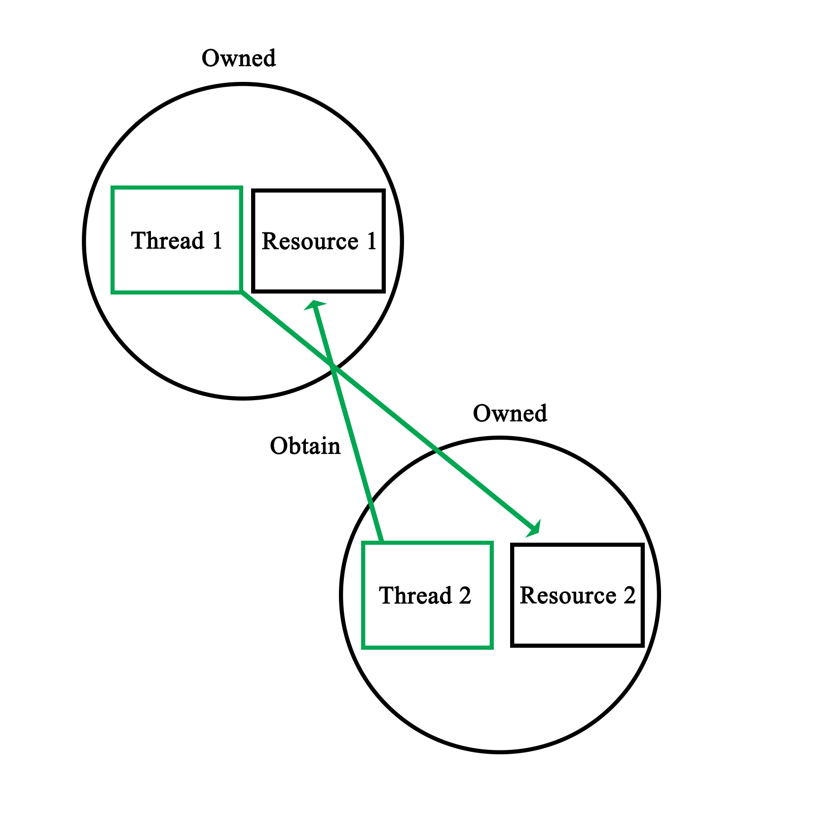
This makes it clear that two basic rules when it comes to preventing deadlocks are:
We saw a real-life example of this in Chapter 11, Thread Synchronization and Communication, when we looked at the dispatcher demonstration code. This code involves two mutexes, to safe-guard access to two data structures:
void Dispatcher::addRequest(AbstractRequest* request) {
workersMutex.lock();
if (!workers.empty()) {
Worker* worker = workers.front();
worker->setRequest(request);
condition_variable* cv;
mutex* mtx;
worker->getCondition(cv);
worker->getMutex(mtx);
unique_lock<mutex> lock(*mtx);
cv->notify_one();
workers.pop();
workersMutex.unlock();
}
else {
workersMutex.unlock();
requestsMutex.lock();
requests.push(request);
requestsMutex.unlock();
}
}
The mutexes here are the workersMutex and requestsMutex variables. We can clearly see how at no point do we hold onto a mutex before trying to obtain access to the other one. We explicitly lock the workersMutex at the beginning of the method, so that we can safely check whether the workers data structure is empty or not.
If it's not empty, we hand the new request to a worker. Then, as we are done with the workers, data structure, we release the mutex. At this point, we retain zero mutexes. Nothing too complex here, as we just use a single mutex.
The interesting thing is in the else statement, for when there is no waiting worker and we need to obtain the second mutex. As we enter this scope, we retain one mutex. We could just attempt to obtain the requestsMutex and assume that it will work, yet this may deadlock, for this simple reason:
bool Dispatcher::addWorker(Worker* worker) {
bool wait = true;
requestsMutex.lock();
if (!requests.empty()) {
AbstractRequest* request = requests.front();
worker->setRequest(request);
requests.pop();
wait = false;
requestsMutex.unlock();
}
else {
requestsMutex.unlock();
workersMutex.lock();
workers.push(worker);
workersMutex.unlock();
}
return wait;
}
The accompanying function to the earlier preceding function we see also uses these two mutexes. Worse, this function runs in a separate thread. As a result, when the first function holds the workersMutex as it tries to obtain the requestsMutex, with this second function simultaneously holding the latter, while trying to obtain the former, we hit a deadlock.
In the functions, as we see them here, however, both rules have been implemented successfully; we never hold more than one lock at a time, and we release any locks we hold as soon as we can. This can be seen in both else cases, where as we enter them, we first release any locks we do not need any more.
As in either case, we do not need to check respectively, the workers or requests data structures any more; we can release the relevant lock before we do anything else. This results in the following visualization:
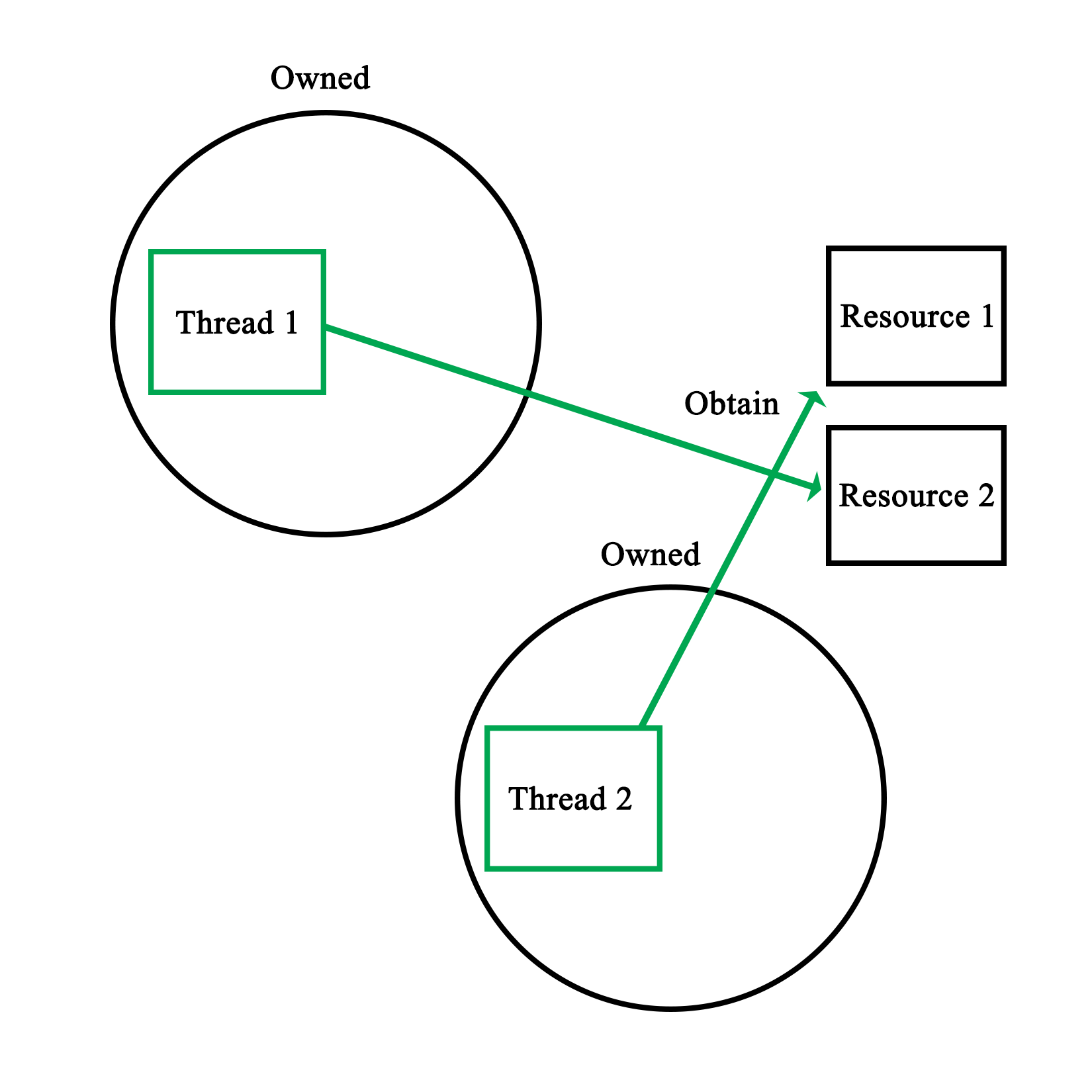
It is of course possible that we may need to use data contained in two or more data structures or variables; data which is used by other threads simultaneously. It may be difficult to ensure that there is no chance of a deadlock in the resulting code.
Here, one may want to consider using temporary variables or similar. By locking the mutex, copying the relevant data, and immediately releasing the lock, there is no chance of deadlock with that mutex. Even if one has to write back results to the data structure, this can be done in a separate action.
This adds two more rules in preventing deadlocks:
A data race, also known as a race condition, occurs when two or more threads attempt to write to the same shared memory simultaneously. As a result, the state of the shared memory during and at the end of the sequence of instructions executed by each thread is by definition, non-deterministic.
As we saw in Chapter 13, Debugging Multithreaded Code, data races are reported quite often by tools used to debug multi-threaded applications. For example:
==6984== Possible data race during write of size 1 at 0x5CD9260 by thread #1
==6984== Locks held: none
==6984== at 0x40362C: Worker::stop() (worker.h:37)
==6984== by 0x403184: Dispatcher::stop() (dispatcher.cpp:50)
==6984== by 0x409163: main (main.cpp:70)
==6984==
==6984== This conflicts with a previous read of size 1 by thread #2
==6984== Locks held: none
==6984== at 0x401E0E: Worker::run() (worker.cpp:51)
==6984== by 0x408FA4: void std::_Mem_fn_base<void (Worker::*)(), true>::operator()<, void>(Worker*) const (in /media/sf_Projects/Cerflet/dispatcher/dispatcher_demo)
==6984== by 0x408F38: void std::_Bind_simple<std::_Mem_fn<void (Worker::*)()> (Worker*)>::_M_invoke<0ul>(std::_Index_tuple<0ul>) (functional:1531)
==6984== by 0x408E3F: std::_Bind_simple<std::_Mem_fn<void (Worker::*)()> (Worker*)>::operator()() (functional:1520)
==6984== by 0x408D47: std::thread::_Impl<std::_Bind_simple<std::_Mem_fn<void (Worker::*)()> (Worker*)> >::_M_run() (thread:115)
==6984== by 0x4EF8C7F: ??? (in /usr/lib/x86_64-linux-gnu/libstdc++.so.6.0.21)
==6984== by 0x4C34DB6: ??? (in /usr/lib/valgrind/vgpreload_helgrind-amd64-linux.so)
==6984== by 0x53DF6B9: start_thread (pthread_create.c:333)
==6984== Address 0x5cd9260 is 96 bytes inside a block of size 104 alloc'd
==6984== at 0x4C2F50F: operator new(unsigned long) (in /usr/lib/valgrind/vgpreload_helgrind-amd64-linux.so)
==6984== by 0x40308F: Dispatcher::init(int) (dispatcher.cpp:38)
==6984== by 0x4090A0: main (main.cpp:51)
==6984== Block was alloc'd by thread #1
The code which generated the preceding warning was the following:
bool Dispatcher::stop() {
for (int i = 0; i < allWorkers.size(); ++i) {
allWorkers[i]->stop();
}
cout << "Stopped workers.n";
for (int j = 0; j < threads.size(); ++j) {
threads[j]->join();
cout << "Joined threads.n";
}
}
Consider this code in the Worker instance:
void stop() { running = false; }
We also have:
void Worker::run() {
while (running) {
if (ready) {
ready = false;
request->process();
request->finish();
}
if (Dispatcher::addWorker(this)) {
while (!ready && running) {
unique_lock<mutex> ulock(mtx);
if (cv.wait_for(ulock, chrono::seconds(1)) == cv_status::timeout) {
}
}
}
}
}
Here, running is a Boolean variable that is being set to false (writing to it from one thread), signaling the worker thread that it should terminate its waiting loop, where reading the Boolean variable is done from a different process, the main thread versus the worker thread:
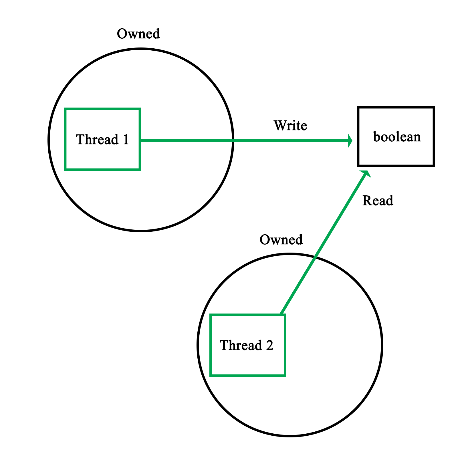
This particular example's warning was due to a Boolean variable being simultaneously written and read. Naturally, the reason why this specific situation is safe has to do with atomics, as explained in detail in Chapter 15, Atomic Operations - Working with the Hardware.
The reason why even an operation like this is potentially risky is because the reading operation may occur while the variable is still in the process of being updated. In the case of, for example, a 32-bit integer, depending on the hardware architecture, updating this variable might be done in one operation, or multiple. In the latter case, the reading operation might read an intermediate value with unpredictable results:
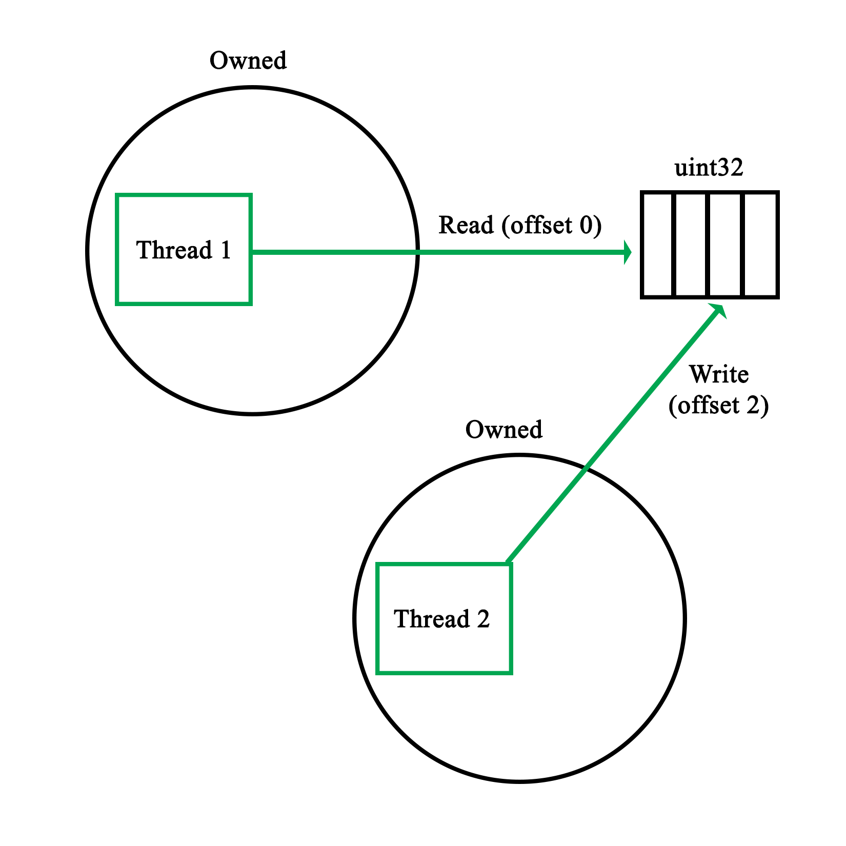
A more comical situation occurs when multiple threads write to a standard with out using, for example, cout. As this stream is not thread-safe, the resulting output stream will contain bits and pieces of the input streams, from whenever either of the threads got a chance to write:
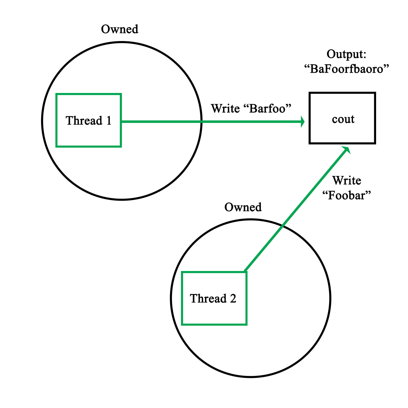
The basic rules to prevent data races thus are:
This essentially means that any write or read has to be thread-safe. If one writes to shared memory, no other thread should be able to write to it at the same time. Similarly, when we read from a shared resource, we need to ensure that, at most, only other threads are also reading the shared resource.
This level of mutual exclusion is naturally accomplished by mutexes as we have seen in the preceding chapters, with a refinement offered in read-write locks, which allows for simultaneous readers while having writes as fully mutually exclusive events.
Of course, there are also gotchas with mutexes, as we will see in the following section.
Mutexes form the basis of practically all forms of mutual exclusion APIs. At their core, they seem extremely simple, only one thread can own a mutex, with other threads neatly waiting in a queue until they can obtain the lock on the mutex.
One might even picture this process as follows:
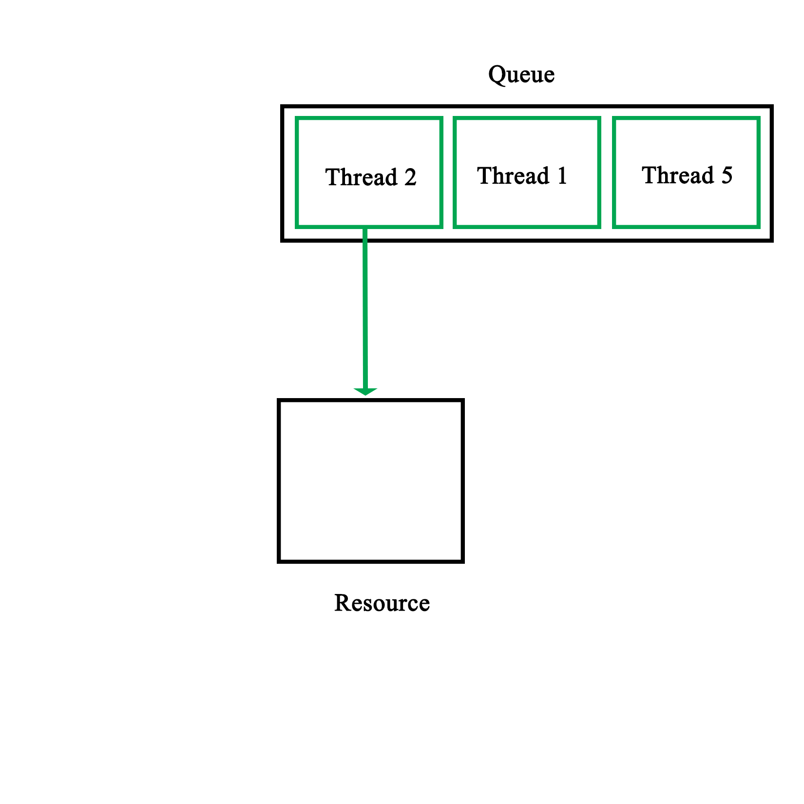
The reality is of course less pretty, mostly owing to the practical limitations imposed on us by the hardware. One obvious limitation is that synchronization primitives aren't free. Even though they are implemented in the hardware, it takes multiple calls to make them work.
The two most common ways to implement mutexes in the hardware is to use either the test-and-set (TAS) or compare-and-swap (CAS) CPU features.
Test-and-set is usually implemented as two assembly-level instructions, which are executed autonomously, meaning that they cannot be interrupted. The first instruction tests whether a certain memory area is set to a 1 or zero. The second instruction is executed only when the value is a zero (false). This means that the mutex was not locked yet. The second instruction thus sets the memory area to a 1, locking the mutex.
In pseudo-code, this would look like this:
bool TAS(bool lock) {
if (lock) {
return true;
}
else {
lock = true;
return false;
}
}
Compare-and-swap is a lesser used variation on this, which performs a comparison operation on a memory location and a given value, only replacing the contents of that memory location if the first two match:
bool CAS(int* p, int old, int new) {
if (*p != old) {
return false;
}
*p = new;
return true;
}
In either case, one would have to actively repeat either function until a positive value is returned:
volatile bool lock = false;
void critical() {
while (TAS(&lock) == false);
// Critical section
lock = 0;
}
Here, a simple while loop is used to constantly poll the memory area (marked as volatile to prevent possibly problematic compiler optimizations). Generally, an algorithm is used for this which slowly reduces the rate at which it is being polled. This is to reduce the amount of pressure on the processor and memory systems.
This makes it clear that the use of a mutex is not free, but that each thread which waits for a mutex lock actively uses resources. As a result, the general rules here are:
As we saw earlier in the section on mutexes, there are some issues to keep in mind when using mutexes. Naturally these also apply when using locks and other mechanisms based on mutexes, even if some of these issues are smoothed over by these APIs.
One of the things one may get confused about when first using multithreading APIs is what the actual difference is between the different synchronization types. As we covered earlier in this chapter, mutexes underlie virtually all synchronization mechanisms, merely differing in the way that they use mutexes to implement the provided functionality.
The important thing here is that they are not distinct synchronization mechanisms, but merely specializations of the basic mutex type. Whether one would use a regular mutex, a read/write lock, a semaphore - or even something as esoteric as a reentrant (recursive) mutex or lock - depends fully on the particular problem which one is trying to solve.
For the scheduler, we first encountered in Chapter 11, Thread Synchronization and Communication, we used regular mutexes to protect the data structures containing the queued worker threads and requests. Since any access of either data structure would likely not only involve reading actions, but also the manipulation of the structure, it would not make sense there to use read/write locks. Similarly, recursive locks would not serve any purpose over the humble mutex.
For each synchronization problem, one therefore has to ask the following questions:
It's therefore attractive to go for a complex type, but generally it's best to stick with the simpler type which fulfills all the requirements. When it comes to debugging one's implementation, precious time can be saved over a fancier implementation.
Recently it has become popular to advise against the use of threads, instead advocating the use of other asynchronous processing mechanisms, such as promise. The reasons behind this are that the use of threads and the synchronization involved is complex and error-prone. Often one just wants to run a task in parallel and not concern oneself with how the result is obtained.
For simple tasks which would run only briefly, this can certainly make sense. The main advantage of a thread-based implementation will always be that one can fully customize its behavior. With a promise, one sends in a task to run and at the end, one gets the result out of a future instance. This is convenient for simple tasks, but obviously does not cover a lot of situations.
The best approach here is to first learn threads and synchronization mechanisms well, along with their limitations. Only after that does it really make sense to consider whether one wishes to use a promise, packaged_task, or a full-blown thread.
Another major consideration with these fancier, future-based APIs is that they are heavily template-based, which can make the debugging and troubleshooting of any issues which may occur significantly less easy than when using the more straightforward and low-level APIs.
Static variables are variables which are declared only once, essentially existing in a global scope, though potentially only shared between instances of a particular class. It's also possible to have classes which are completely static:
class Foo {
static std::map<int, std::string> strings;
static std::string oneString;
public:
static void init(int a, std::string b, std::string c) {
strings.insert(std::pair<int, std::string>(a, b));
oneString = c;
}
};
std::map<int, std::string> Foo::strings;
std::string Foo::oneString;
As we can see here, static variables along with static functions seem like a very simple, yet powerful concept. While at its core this is true, there's a major issue which will catch the unwary when it comes to static variables and the initialization of classes. This is in the form of initialization order.
Imagine what happens if we wish to use the preceding class from another class' static initialization, like this:
class Bar {
static std::string name;
static std::string initName();
public:
void init();
};
// Static initializations.
std::string Bar::name = Bar::initName();
std::string Bar::initName() {
Foo::init(1, "A", "B");
return "Bar";
}
While this may seem like it would work fine, adding the first string to the class' map structure with the integer as key means there is a very good chance that this code will crash. The reason for this is simple, there is no guarantee that Foo::string is initialized at the point when we call Foo::init(). Trying to use an uninitialized map structure will thus lead to an exception.
In short, the initialization order of static variables is basically random, leading to non-deterministic behavior if this is not taken into account.
The solution to this problem is fairly simple. Basically, the goal is to make the initialization of more complex static variables explicit instead of implicit like in the preceding example. For this we modify the Foo class:
class Foo {
static std::map<int, std::string>& strings();
static std::string oneString;
public:
static void init(int a, std::string b, std::string c) {
static std::map<int, std::string> stringsStatic = Foo::strings();
stringsStatic.insert(std::pair<int, std::string>(a, b));
oneString = c;
}
};
std::string Foo::oneString;
std::map<int, std::string>& Foo::strings() {
static std::map<int, std::string>* stringsStatic = new std::map<int, std::string>();
return *stringsStatic;
}
Starting at the top, we see that we no longer define the static map directly. Instead, we have a private function with the same name. This function's implementation is found at the bottom of this sample code. In it, we have a static pointer to a map structure with the familiar map definition.
When this function is called, a new map is created when there's no instance yet, due to it being a static variable. In the modified init() function, we see that we call the strings() function to obtain a reference to this instance. This is the explicit initialization part, as calling the function will always ensure that the map structure is initialized before we use it, solving the earlier problem we had.
We also see a small optimization here: the stringsStatic variable we create is also static, meaning that we will only ever call the strings() function once. This makes repeated function calls unnecessary and regains the speed we would have had with the previous simple--but unstable--implementation.
The essential rule with static variable initialization is thus, always use explicit initialization for non-trivial static variables.
In this chapter, we looked at a number of good practices and rules to keep in mind when writing multithreaded code, along with some general advice. At this point, one should be able to avoid some of the bigger pitfalls and major sources of confusion when writing such code.
In the next chapter, we will be looking at how to use the underlying hardware to our advantage with atomic operations, along with the <atomics> header that was also introduced with C++11.
A lot of optimization and thread-safety depends on one's understanding of the underlying hardware: from aligned memory access on some architectures, to knowing which data sizes and thus C++ types can be safely addressed without performance penalties or the need for mutexes and similar.
This chapter looks at how one can make use of the characteristics of a number of processor architectures in order to, for example, prevent the use of mutexes where atomic operations would prevent any access conflicts regardless. Compiler-specific extensions such as those in GCC are also examined.
Topics in this chapter include:
Briefly put, an atomic operation is an operation which the processor can execute with a single instruction. This makes it atomic in the sense that nothing (barring interrupts) can interfere with it, or change any variables or data it may be using.
Applications include guaranteeing the order of instruction execution, lock-free implementations, and related uses where instruction execution order and memory access guarantees are important.
Before the 2011 C++ standard, the access to such atomic operations as provided by the processor was only provided by the compiler, using extensions.
For Microsoft's MSVC compiler there are the interlocked functions, as summarized from the MSDN documentation, starting with the adding features:
|
Interlocked function |
Description |
|
InterlockedAdd |
Performs an atomic addition operation on the specified LONG values. |
|
InterlockedAddAcquire |
Performs an atomic addition operation on the specified LONG values. The operation is performed with acquire memory ordering semantics. |
|
InterlockedAddRelease |
Performs an atomic addition operation on the specified LONG values. The operation is performed with release memory ordering semantics. |
|
InterlockedAddNoFence |
Performs an atomic addition operation on the specified LONG values. The operation is performed atomically, but without using memory barriers (covered in this chapter). |
These are the 32-bit versions of this feature. There are also 64-bit versions of this and other methods in the API. Atomic functions tend to be focused on a specific variable type, but variations in this API have been left out of this summary to keep it brief.
We can also see the acquire and release variations. These provide the guarantee that the respective read or write access will be protected from memory reordering (on a hardware level) with any subsequent read or write operation. Finally, the no fence variation (also known as a memory barrier) performs the operation without the use of any memory barriers.
Normally CPUs perform instructions (including memory reads and writes) out of order to optimize performance. Since this type of behavior is not always desirable, memory barriers were added to prevent this instruction reordering.
Next is the atomic AND feature:
|
Interlocked function |
Description |
|
InterlockedAnd |
Performs an atomic AND operation on the specified LONG values. |
|
InterlockedAndAcquire |
Performs an atomic AND operation on the specified LONG values. The operation is performed with acquire memory ordering semantics. |
|
InterlockedAndRelease |
Performs an atomic AND operation on the specified LONG values. The operation is performed with release memory ordering semantics. |
|
InterlockedAndNoFence |
Performs an atomic AND operation on the specified LONG values. The operation is performed atomically, but without using memory barriers. |
The bit-test features are as follows:
|
Interlocked function |
Description |
|
InterlockedBitTestAndComplement |
Tests the specified bit of the specified LONG value and complements it. |
|
InterlockedBitTestAndResetAcquire |
Tests the specified bit of the specified LONG value and sets it to 0. The operation is atomic, and it is performed with acquire memory ordering semantics. |
|
InterlockedBitTestAndResetRelease |
Tests the specified bit of the specified LONG value and sets it to 0. The operation is atomic, and it is performed using memory release semantics. |
|
InterlockedBitTestAndSetAcquire |
Tests the specified bit of the specified LONG value and sets it to 1. The operation is atomic, and it is performed with acquire memory ordering semantics. |
|
InterlockedBitTestAndSetRelease |
Tests the specified bit of the specified LONG value and sets it to 1. The operation is atomic, and it is performed with release memory ordering semantics. |
|
InterlockedBitTestAndReset |
Tests the specified bit of the specified LONG value and sets it to 0. |
|
InterlockedBitTestAndSet |
Tests the specified bit of the specified LONG value and sets it to 1. |
The comparison features can be listed as shown:
|
Interlocked function |
Description |
|
InterlockedCompareExchange |
Performs an atomic compare-and-exchange operation on the specified values. The function compares two specified 32-bit values and exchanges with another 32-bit value based on the outcome of the comparison. |
|
InterlockedCompareExchangeAcquire |
Performs an atomic compare-and-exchange operation on the specified values. The function compares two specified 32-bit values and exchanges with another 32-bit value based on the outcome of the comparison. The operation is performed with acquire memory ordering semantics. |
|
InterlockedCompareExchangeRelease |
Performs an atomic compare-and-exchange operation on the specified values. The function compares two specified 32-bit values and exchanges with another 32-bit value based on the outcome of the comparison. The exchange is performed with release memory ordering semantics. |
|
InterlockedCompareExchangeNoFence |
Performs an atomic compare-and-exchange operation on the specified values. The function compares two specified 32-bit values and exchanges with another 32-bit value based on the outcome of the comparison. The operation is performed atomically, but without using memory barriers. |
|
InterlockedCompareExchangePointer |
Performs an atomic compare-and-exchange operation on the specified pointer values. The function compares two specified pointer values and exchanges with another pointer value based on the outcome of the comparison. |
|
InterlockedCompareExchangePointerAcquire |
Performs an atomic compare-and-exchange operation on the specified pointer values. The function compares two specified pointer values and exchanges with another pointer value based on the outcome of the comparison. The operation is performed with acquire memory ordering semantics. |
|
InterlockedCompareExchangePointerRelease |
Performs an atomic compare-and-exchange operation on the specified pointer values. The function compares two specified pointer values and exchanges with another pointer value based on the outcome of the comparison. The operation is performed with release memory ordering semantics. |
|
InterlockedCompareExchangePointerNoFence |
Performs an atomic compare-and-exchange operation on the specified values. The function compares two specified pointer values and exchanges with another pointer value based on the outcome of the comparison. The operation is performed atomically, but without using memory barriers |
The decrement features are:
|
Interlocked function |
Description |
|
InterlockedDecrement |
Decrements (decreases by one) the value of the specified 32-bit variable as an atomic operation. |
|
InterlockedDecrementAcquire |
Decrements (decreases by one) the value of the specified 32-bit variable as an atomic operation. The operation is performed with acquire memory ordering semantics. |
|
InterlockedDecrementRelease |
Decrements (decreases by one) the value of the specified 32-bit variable as an atomic operation. The operation is performed with release memory ordering semantics. |
|
InterlockedDecrementNoFence |
Decrements (decreases by one) the value of the specified 32-bit variable as an atomic operation. The operation is performed atomically, but without using memory barriers. |
The exchange (swap) features are:
|
Interlocked function |
Description |
|
InterlockedExchange |
Sets a 32-bit variable to the specified value as an atomic operation. |
|
InterlockedExchangeAcquire |
Sets a 32-bit variable to the specified value as an atomic operation. The operation is performed with acquire memory ordering semantics. |
|
InterlockedExchangeNoFence |
Sets a 32-bit variable to the specified value as an atomic operation. The operation is performed atomically, but without using memory barriers. |
|
InterlockedExchangePointer |
Atomically exchanges a pair of pointer values. |
|
InterlockedExchangePointerAcquire |
Atomically exchanges a pair of pointer values. The operation is performed with acquire memory ordering semantics. |
|
InterlockedExchangePointerNoFence |
Atomically exchanges a pair of addresses. The operation is performed atomically, but without using memory barriers. |
|
InterlockedExchangeSubtract |
Performs an atomic subtraction of two values. |
|
InterlockedExchangeAdd |
Performs an atomic addition of two 32-bit values. |
|
InterlockedExchangeAddAcquire |
Performs an atomic addition of two 32-bit values. The operation is performed with acquire memory ordering semantics. |
|
InterlockedExchangeAddRelease |
Performs an atomic addition of two 32-bit values. The operation is performed with release memory ordering semantics. |
|
InterlockedExchangeAddNoFence |
Performs an atomic addition of two 32-bit values. The operation is performed atomically, but without using memory barriers. |
The increment features are:
|
Interlocked function |
Description |
|
InterlockedIncrement |
Increments (increases by one) the value of the specified 32-bit variable as an atomic operation. |
|
InterlockedIncrementAcquire |
Increments (increases by one) the value of the specified 32-bit variable as an atomic operation. The operation is performed using acquire memory ordering semantics. |
|
InterlockedIncrementRelease |
Increments (increases by one) the value of the specified 32-bit variable as an atomic operation. The operation is performed using release memory ordering semantics. |
|
InterlockedIncrementNoFence |
Increments (increases by one) the value of the specified 32-bit variable as an atomic operation. The operation is performed atomically, but without using memory barriers. |
The OR feature:
|
Interlocked function |
Description |
|
InterlockedOr |
Performs an atomic OR operation on the specified LONG values. |
|
InterlockedOrAcquire |
Performs an atomic OR operation on the specified LONG values. The operation is performed with acquire memory ordering semantics. |
|
InterlockedOrRelease |
Performs an atomic OR operation on the specified LONG values. The operation is performed with release memory ordering semantics. |
|
InterlockedOrNoFence |
Performs an atomic OR operation on the specified LONG values. The operation is performed atomically, but without using memory barriers. |
Finally, the exclusive OR (XOR) features are:
|
Interlocked function |
Description |
|
InterlockedXor |
Performs an atomic XOR operation on the specified LONG values. |
|
InterlockedXorAcquire |
Performs an atomic XOR operation on the specified LONG values. The operation is performed with acquire memory ordering semantics. |
|
InterlockedXorRelease |
Performs an atomic XOR operation on the specified LONG values. The operation is performed with release memory ordering semantics. |
|
InterlockedXorNoFence |
Performs an atomic XOR operation on the specified LONG values. The operation is performed atomically, but without using memory barriers. |
Like Visual C++, GCC also comes with a set of built-in atomic functions. These differ based on the underlying architecture that the GCC version and the standard library one uses. Since GCC is used on a considerably larger number of platforms and operating systems than VC++, this is definitely a big factor when considering portability.
For example, not every built-in atomic function provided on the x86 platform will be available on ARM, partially due to architectural differences, including variations of the specific ARM architecture. For example, ARMv6, ARMv7, or the current ARMv8, along with the Thumb instruction set, and so on.
Before the C++11 standard, GCC used __sync-prefixed extensions for atomics:
type __sync_fetch_and_add (type *ptr, type value, ...) type __sync_fetch_and_sub (type *ptr, type value, ...) type __sync_fetch_and_or (type *ptr, type value, ...) type __sync_fetch_and_and (type *ptr, type value, ...) type __sync_fetch_and_xor (type *ptr, type value, ...) type __sync_fetch_and_nand (type *ptr, type value, ...)
These operations fetch a value from memory and perform the specified operation on it, returning the value that was in memory. These all use a memory barrier.
type __sync_add_and_fetch (type *ptr, type value, ...) type __sync_sub_and_fetch (type *ptr, type value, ...) type __sync_or_and_fetch (type *ptr, type value, ...) type __sync_and_and_fetch (type *ptr, type value, ...) type __sync_xor_and_fetch (type *ptr, type value, ...) type __sync_nand_and_fetch (type *ptr, type value, ...)
These operations are similar to the first set, except they return the new value after the specified operation.
bool __sync_bool_compare_and_swap (type *ptr, type oldval, type newval, ...) type __sync_val_compare_and_swap (type *ptr, type oldval, type newval, ...)
These comparison operations will write the new value if the old value matches the provided value. The Boolean variation returns true if the new value has been written.
__sync_synchronize (...)
This function creates a full memory barrier.
type __sync_lock_test_and_set (type *ptr, type value, ...)
This method is actually an exchange operation unlike what the name suggests. It updates the pointer value and returns the previous value. This uses not a full memory barrier, but an acquire barrier, meaning that it does not release the barrier.
void __sync_lock_release (type *ptr, ...)
This function releases the barrier obtained by the previous method.
To adapt to the C++11 memory model, GCC added the __atomic built-in methods, which also changes the API considerably:
type __atomic_load_n (type *ptr, int memorder) void __atomic_load (type *ptr, type *ret, int memorder) void __atomic_store_n (type *ptr, type val, int memorder) void __atomic_store (type *ptr, type *val, int memorder) type __atomic_exchange_n (type *ptr, type val, int memorder) void __atomic_exchange (type *ptr, type *val, type *ret, int memorder) bool __atomic_compare_exchange_n (type *ptr, type *expected, type desired, bool weak, int success_memorder, int failure_memorder) bool __atomic_compare_exchange (type *ptr, type *expected, type *desired, bool weak, int success_memorder, int failure_memorder)
First are the generic load, store, and exchange functions. They are fairly self-explanatory. Load functions read a value in memory, store functions store a value in memory, and exchange functions swap the existing value with a new value. Compare and exchange functions make the swapping conditional.
type __atomic_add_fetch (type *ptr, type val, int memorder) type __atomic_sub_fetch (type *ptr, type val, int memorder) type __atomic_and_fetch (type *ptr, type val, int memorder) type __atomic_xor_fetch (type *ptr, type val, int memorder) type __atomic_or_fetch (type *ptr, type val, int memorder) type __atomic_nand_fetch (type *ptr, type val, int memorder)
These functions are essentially the same as in the old API, returning the result of the specific operation.
type __atomic_fetch_add (type *ptr, type val, int memorder) type __atomic_fetch_sub (type *ptr, type val, int memorder) type __atomic_fetch_and (type *ptr, type val, int memorder) type __atomic_fetch_xor (type *ptr, type val, int memorder) type __atomic_fetch_or (type *ptr, type val, int memorder) type __atomic_fetch_nand (type *ptr, type val, int memorder)
And again, the same functions, updated for the new API. These return the original value (fetch before operation).
bool __atomic_test_and_set (void *ptr, int memorder)
Unlike the similarly named function in the old API, this function performs a real test and set operation instead of the exchange operation of the old API's function, which still requires one to release the memory barrier afterwards. The test is for some defined value.
void __atomic_clear (bool *ptr, int memorder)
This function clears the pointer address, setting it to 0.
void __atomic_thread_fence (int memorder)
A synchronization memory barrier (fence) between threads can be created using this function.
void __atomic_signal_fence (int memorder)
This function creates a memory barrier between a thread and signal handlers within that same thread.
bool __atomic_always_lock_free (size_t size, void *ptr)
The function checks whether objects of the specified size will always create lock-free atomic instructions for the current processor architecture.
bool __atomic_is_lock_free (size_t size, void *ptr)
This is essentially the same as the previous function.
Memory barriers (fences) are not always used in the C++11 memory model for atomic operations. In the GCC built-in atomics API, this is reflected in the memorder parameter in its functions. The possible values for this map directly to the values in the C++11 atomics API:
The preceding list was copied from the GCC manual's chapter on atomics for GCC 7.1. Along with the comments in that chapter, it makes it quite clear that trade-offs were made when implementing both the C++11 atomics support within its memory model and in the compiler's implementation.
Since atomics rely on the underlying hardware support, there will never be a single piece of code using atomics that will work across a wide variety of architectures.
There are many more compiler toolchains for C/C++ than just VC++ and GCC, of course, including the Intel Compiler Collection (ICC) and other, usually proprietary tools.. These all have their own collection of built-in atomic functions. Fortunately, thanks to the C++11 standard, we now have a fully portable standard for atomics between compilers. Generally, this means that outside of very specific use cases (or maintenance of existing code), one would use the C++ standard over compiler-specific extensions.
In order to use the native C++11 atomics features, all one has to do is include the <atomic> header. This makes available the atomic class, which uses templates to adapt itself to the required type, with a large number of predefined typedefs:
|
Typedef name |
Full specialization |
|
std::atomic_bool |
std::atomic<bool> |
|
std::atomic_char |
std::atomic<char> |
|
std::atomic_schar |
std::atomic<signed char> |
|
std::atomic_uchar |
std::atomic<unsigned char> |
|
std::atomic_short |
std::atomic<short> |
|
std::atomic_ushort |
std::atomic<unsigned short> |
|
std::atomic_int |
std::atomic<int> |
|
std::atomic_uint |
std::atomic<unsigned int> |
|
std::atomic_long |
std::atomic<long> |
|
std::atomic_ulong |
std::atomic<unsigned long> |
|
std::atomic_llong |
std::atomic<long long> |
|
std::atomic_ullong |
std::atomic<unsigned long long> |
|
std::atomic_char16_t |
std::atomic<char16_t> |
|
std::atomic_char32_t |
std::atomic<char32_t> |
|
std::atomic_wchar_t |
std::atomic<wchar_t> |
|
std::atomic_int8_t |
std::atomic<std::int8_t> |
|
std::atomic_uint8_t |
std::atomic<std::uint8_t> |
|
std::atomic_int16_t |
std::atomic<std::int16_t> |
|
std::atomic_uint16_t |
std::atomic<std::uint16_t> |
|
std::atomic_int32_t |
std::atomic<std::int32_t> |
|
std::atomic_uint32_t |
std::atomic<std::uint32_t> |
|
std::atomic_int64_t |
std::atomic<std::int64_t> |
|
std::atomic_uint64_t |
std::atomic<std::uint64_t> |
|
std::atomic_int_least8_t |
std::atomic<std::int_least8_t> |
|
std::atomic_uint_least8_t |
std::atomic<std::uint_least8_t> |
|
std::atomic_int_least16_t |
std::atomic<std::int_least16_t> |
|
std::atomic_uint_least16_t |
std::atomic<std::uint_least16_t> |
|
std::atomic_int_least32_t |
std::atomic<std::int_least32_t> |
|
std::atomic_uint_least32_t |
std::atomic<std::uint_least32_t> |
|
std::atomic_int_least64_t |
std::atomic<std::int_least64_t> |
|
std::atomic_uint_least64_t |
std::atomic<std::uint_least64_t> |
|
std::atomic_int_fast8_t |
std::atomic<std::int_fast8_t> |
|
std::atomic_uint_fast8_t |
std::atomic<std::uint_fast8_t> |
|
std::atomic_int_fast16_t |
std::atomic<std::int_fast16_t> |
|
std::atomic_uint_fast16_t |
std::atomic<std::uint_fast16_t> |
|
std::atomic_int_fast32_t |
std::atomic<std::int_fast32_t> |
|
std::atomic_uint_fast32_t |
std::atomic<std::uint_fast32_t> |
|
std::atomic_int_fast64_t |
std::atomic<std::int_fast64_t> |
|
std::atomic_uint_fast64_t |
std::atomic<std::uint_fast64_t> |
|
std::atomic_intptr_t |
std::atomic<std::intptr_t> |
|
std::atomic_uintptr_t |
std::atomic<std::uintptr_t> |
|
std::atomic_size_t |
std::atomic<std::size_t> |
|
std::atomic_ptrdiff_t |
std::atomic<std::ptrdiff_t> |
|
std::atomic_intmax_t |
std::atomic<std::intmax_t> |
|
std::atomic_uintmax_t |
std::atomic<std::uintmax_t> |
This atomic class defines the following generic functions:
|
Function |
Description |
|
operator= |
Assigns a value to an atomic object. |
|
is_lock_free |
Returns true if the atomic object is lock-free. |
|
store |
Replaces the value of the atomic object with a non-atomic argument, atomically. |
|
load |
Atomically obtains the value of the atomic object. |
|
operator T |
Loads a value from an atomic object. |
|
exchange |
Atomically replaces the value of the object with the new value and returns the old value. |
|
compare_exchange_weak compare_exchange_strong |
Atomically compares the value of the object and swaps values if equal, or else returns the current value. |
With the C++17 update, the is_always_lock_free constant is added. This allows one to inquire whether the type is always lock-free.
Finally, we have the specialized atomic functions:
|
Function |
Description |
|
fetch_add |
Atomically adds the argument to the value stored in the atomic object and returns the old value. |
|
fetch_sub |
Atomically subtracts the argument from the value stored in the atomic object and returns the old value. |
|
fetch_and |
Atomically performs bitwise AND between the argument and the value of the atomic object and returns the old value. |
|
fetch_or |
Atomically performs bitwise OR between the argument and the value of the atomic object and returns the old value. |
|
fetch_xor |
Atomically performs bitwise XOR between the argument and the value of the atomic object and returns the old value. |
|
operator++ operator++(int) operator-- operator--(int) |
Increments or decrements the atomic value by one. |
|
operator+= operator-= operator&= operator|= operator^= |
Adds, subtracts, or performs a bitwise AND, OR, XOR operation with the atomic value. |
A basic example using fetch_add would look like this:
#include <iostream>
#include <thread>
#include <atomic>
std::atomic<long long> count;
void worker() {
count.fetch_add(1, std::memory_order_relaxed);
}
int main() {
std::thread t1(worker);
std::thread t2(worker);
std::thread t3(worker);
std::thread t4(worker);
std::thread t5(worker);
t1.join();
t2.join();
t3.join();
t4.join();
t5.join();
std::cout << "Count value:" << count << 'n';
}
The result of this example code would be 5. As we can see here, we can implement a basic counter this way with atomics, instead of having to use any mutexes or similar in order to provide thread synchronization.
In addition to the atomic class, there are also a number of template-based functions defined in the <atomic> header which we can use in a manner more akin to the compiler's built-in atomic functions:
|
Function |
Description |
|
atomic_is_lock_free |
Checks whether the atomic type's operations are lock-free. |
|
atomic_storeatomic_store_explicit |
Atomically replaces the value of the atomic object with a non-atomic argument. |
|
atomic_load atomic_load_explicit |
Atomically obtains the value stored in an atomic object. |
|
atomic_exchange atomic_exchange_explicit |
Atomically replaces the value of the atomic object with a non-atomic argument and returns the old value of atomic. |
|
atomic_compare_exchange_weak atomic_compare_exchange_weak_explicit atomic_compare_exchange_strong atomic_compare_exchange_strong_explicit |
Atomically compares the value of the atomic object with a non-atomic argument and performs an atomic exchange if equal or atomic load if not. |
|
atomic_fetch_add atomic_fetch_add_explicit |
Adds a non-atomic value to an atomic object and obtains the previous value of atomic. |
|
atomic_fetch_sub atomic_fetch_sub_explicit |
Subtracts a non-atomic value from an atomic object and obtains the previous value of atomic. |
|
atomic_fetch_and atomic_fetch_and_explicit |
Replaces the atomic object with the result of logical AND with a non-atomic argument and obtains the previous value of the atomic. |
|
atomic_fetch_or atomic_fetch_or_explicit |
Replaces the atomic object with the result of logical OR with a non-atomic argument and obtains the previous value of atomic. |
|
atomic_fetch_xor atomic_fetch_xor_explicit |
Replaces the atomic object with the result of logical XOR with a non-atomic argument and obtains the previous value of atomic. |
|
atomic_flag_test_and_set atomic_flag_test_and_set_explicit |
Atomically sets the flag to true and returns its previous value. |
|
atomic_flag_clear atomic_flag_clear_explicit |
Atomically sets the value of the flag to false. |
|
atomic_init |
Non-atomic initialization of a default-constructed atomic object. |
|
kill_dependency |
Removes the specified object from the std::memory_order_consume dependency tree. |
|
atomic_thread_fence |
Generic memory order-dependent fence synchronization primitive. |
|
atomic_signal_fence |
Fence between a thread and a signal handler executed in the same thread. |
The difference between the regular and explicit functions is that the latter allows one to actually set the memory order to use. The former always uses memory_order_seq_cst as the memory order.
In this example using atomic_fetch_sub, an indexed container is processed by multiple threads concurrently, without the use of locks:
#include <string>
#include <thread>
#include <vector>
#include <iostream>
#include <atomic>
#include <numeric>
const int N = 10000;
std::atomic<int> cnt;
std::vector<int> data(N);
void reader(int id) {
for (;;) {
int idx = atomic_fetch_sub_explicit(&cnt, 1, std::memory_order_relaxed);
if (idx >= 0) {
std::cout << "reader " << std::to_string(id) << " processed item "
<< std::to_string(data[idx]) << 'n';
}
else {
std::cout << "reader " << std::to_string(id) << " done.n";
break;
}
}
}
int main() {
std::iota(data.begin(), data.end(), 1);
cnt = data.size() - 1;
std::vector<std::thread> v;
for (int n = 0; n < 10; ++n) {
v.emplace_back(reader, n);
}
for (std::thread& t : v) {
t.join();
}
}
This example code uses a vector filled with integers of size N as the data source, filling it with 1s. The atomic counter object is set to the size of the data vector. After this, 10 threads are created (initialized in place using the vector's emplace_back C++11 feature), which run the reader function.
In that function, we read the current value of the index counter from memory using the atomic_fetch_sub_explicit function, which allows us to use the memory_order_relaxed memory order. This function also subtracts the value we pass from this old value, counting the index down by 1.
So long as the index number we obtain this way is higher or equal to zero, the function continues, otherwise it will quit. Once all the threads have finished, the application exits.
std::atomic_flag is an atomic Boolean type. Unlike the other specializations of the atomic class, it is guaranteed to be lock-free. It does not however, offer any load or store operations.
Instead, it offers the assignment operator, and functions to either clear, or test_and_set the flag. The former thereby sets the flag to false, and the latter will test and set it to true.
This property is defined as an enumeration in the <atomic> header:
enum memory_order {
memory_order_relaxed,
memory_order_consume,
memory_order_acquire,
memory_order_release,
memory_order_acq_rel,
memory_order_seq_cst
};
In the GCC section, we already touched briefly on the topic of memory order. As mentioned there, this is one of the parts where the characteristics of the underlying hardware architecture surface somewhat.
Basically, memory order determines how non-atomic memory accesses are to be ordered (memory access order) around an atomic operation. What this affects is how different threads will see the data in memory as they're executing their instructions:
|
Enum |
Description |
|
memory_order_relaxed |
Relaxed operation: there are no synchronization or ordering constraints imposed on other reads or writes, only this operation's atomicity is guaranteed. |
|
memory_order_consume |
A load operation with this memory order performs a consume operation on the affected memory location: no reads or writes in the current thread dependent on the value currently loaded can be reordered before this load. Writes to data-dependent variables in other threads that release the same atomic variable are visible in the current thread. On most platforms, this affects compiler optimizations only. |
|
memory_order_acquire |
A load operation with this memory order performs the acquire operation on the affected memory location: no reads or writes in the current thread can be reordered before this load. All writes in other threads that release the same atomic variable are visible in the current thread. |
|
memory_order_release |
A store operation with this memory order performs the release operation: no reads or writes in the current thread can be reordered after this store. All writes in the current thread are visible in other threads that acquire the same atomic variable and writes that carry a dependency into the atomic variable become visible in other threads that consume the same atomic. |
|
memory_order_acq_rel |
A read-modify-write operation with this memory order is both an acquire operation and a release operation. No memory reads or writes in the current thread can be reordered before or after this store. All writes in other threads that release the same atomic variable are visible before the modification and the modification is visible in other threads that acquire the same atomic variable. |
|
memory_order_seq_cst |
Any operation with this memory order is both an acquire operation and a release operation, plus a single total order exists in which all threads observe all modifications in the same order. |
With relaxed memory ordering, no order is enforced among concurrent memory accesses. All that this type of ordering guarantees is atomicity and modification order.
A typical use for this type of ordering is for counters, whether incrementing--or decrementing, as we saw earlier in the example code in the previous section.
If an atomic store in thread A is tagged memory_order_release and an atomic load in thread B from the same variable is tagged memory_order_acquire, all memory writes (non-atomic and relaxed atomic) that happened before the atomic store from the point of view of thread A, become visible side-effects in thread B. That is, once the atomic load has been completed, thread B is guaranteed to see everything thread A wrote to memory.
This type of operation is automatic on so-called strongly ordered architectures, including x86, SPARC, and POWER. Weakly-ordered architectures, such as ARM, PowerPC, and Itanium, will require the use of memory barriers here.
Typical applications of this type of memory ordering include mutual exclusion mechanisms, such as a mutex or atomic spinlock.
If an atomic store in thread A is tagged memory_order_release and an atomic load in thread B from the same variable is tagged memory_order_consume, all memory writes (non-atomic and relaxed atomic) that are dependency-ordered before the atomic store from the point of view of thread A, become visible side-effects within those operations in thread B into which the load operation carries dependency. That is, once the atomic load has been completed, those operators and functions in thread B that use the value obtained from the load are guaranteed to see what thread A wrote to memory.
This type of ordering is automatic on virtually all architectures. The only major exception is the (obsolete) Alpha architecture. A typical use case for this type of ordering would be read access to data that rarely gets changed.
Atomic operations tagged memory_order_seq_cst not only order memory the same way as release/acquire ordering (everything that happened before a store in one thread becomes a visible side effect in the thread that did a load), but also establishes a single total modification order of all atomic operations that are so tagged.
This type of ordering may be necessary for situations where all consumers must observe the changes being made by other threads in exactly the same order. It requires full memory barriers as a consequence on multi-core or multi-CPU systems.
As a result of such a complex setup, this type of ordering is significantly slower than the other types. It also requires that every single atomic operation has to be tagged with this type of memory ordering, or the sequential ordering will be lost.
The volatile keyword is probably quite familiar to anyone who has ever written complex multithreaded code. Its basic use is to tell the compiler that the relevant variable should always be loaded from memory, never making assumptions about its value. It also ensures that the compiler will not make any aggressive optimizations to the variable.
For multithreaded applications, it is generally ineffective, however, its use is discouraged. The main issue with the volatile specification is that it does not define a multithreaded memory model, meaning that the result of this keyword may not be deterministic across platforms, CPUs and even toolchains.
Within the area of atomics, this keyword is not required, and in fact is unlikely to be helpful. To guarantee that one obtains the current version of a variable that is shared between multiple CPU cores and their caches, one would have to use an operation like atomic_compare_exchange_strong, atomic_fetch_add, or atomic_exchange to let the hardware fetch the correct and current value.
For multithreaded code, it is recommended to not use the volatile keyword and use atomics instead, to guarantee proper behavior.
In this chapter, we looked at atomic operations and exactly how they are integrated into compilers to allow one's code to work as closely with the underlying hardware as possible. The reader will now be familiar with the types of atomic operations, the use of a memory barrier (fencing), as well as the various types of memory ordering and their implications.
The reader is now capable of using atomic operations in their own code to accomplish lock-free designs and to make proper use of the C++11 memory model.
In the next chapter, we will take everything we have learned so far and move away from CPUs, instead taking a look at GPGPU, the general-purpose processing of data on video cards (GPUs).
Distributed computing was one of the original applications of multithreaded programming. Back when every personal computer just contained a single processor with a single core, government and research institutions, as well as some companies would have multi-processor systems, often in the form of clusters. These would be capable of multithreaded processing; by splitting tasks across processors, they could speed up various tasks, including simulations, rendering of CGI movies, and the like.
Nowadays virtually every desktop-level or better system has more than a single processor core, and assembling a number of systems together into a cluster is very easy, using cheap Ethernet wiring. Combined with frameworks such as OpenMP and Open MPI, it's quite easy to expand a C++ based (multithreaded) application to run on a distributed system.
Topics in this chapter include:
When it comes to processing large datasets in parallel, it would be ideal if one could take the data, chop it up into lots of small parts, and push it to a lot of threads, thus significantly shortening the total time spent processing the said data.
The idea behind distributed computing is exactly this: on each node in a distributed system one or more instances of our application run, whereby this application can either be single or multithreaded. Due to the overhead of inter-process communication, it's generally more efficient to use a multithreaded application, as well as due to other possible optimizations--courtesy of resource sharing.
If one already has a multithreaded application ready to use, then one can move straight to using MPI to make it work on a distributed system. Otherwise, OpenMP is a compiler extension (for C/C++ and Fortran) which can make it relatively painless to make an application multithreaded without refactoring.
To do this, OpenMP allows one to mark a common code segment, to be executed on all slave threads. A master thread creates a number of slave threads which will concurrently process that same code segment. A basic Hello World OpenMP application looks like this:
/******************************************************************************
* FILE: omp_hello.c
* DESCRIPTION:
* OpenMP Example - Hello World - C/C++ Version
* In this simple example, the master thread forks a parallel region.
* All threads in the team obtain their unique thread number and print it.
* The master thread only prints the total number of threads. Two OpenMP
* library routines are used to obtain the number of threads and each
* thread's number.
* AUTHOR: Blaise Barney 5/99
* LAST REVISED: 04/06/05
******************************************************************************/
#include <omp.h>
#include <stdio.h>
#include <stdlib.h>
int main (int argc, char *argv[]) {
int nthreads, tid;
/* Fork a team of threads giving them their own copies of variables */
#pragma omp parallel private(nthreads, tid) {
/* Obtain thread number */
tid = omp_get_thread_num();
printf("Hello World from thread = %dn", tid);
/* Only master thread does this */
if (tid == 0) {
nthreads = omp_get_num_threads();
printf("Number of threads = %dn", nthreads);
}
} /* All threads join master thread and disband */ }
What one can easily tell from this basic sample is that OpenMP provides a C based API through the <omp.h> header. We can also see the section that will be executed by each thread, as marked by a #pragma omp preprocessor macro.
The advantage of OpenMP over the examples of multithreaded code which we saw in the preceding chapters, is the ease with which a section of code can be marked as being multithreaded without having to make any actual code changes. The obvious limitation that comes with this is that every thread instance will execute the exact same code and further optimization options are limited.
In order to schedule the execution of code on specific nodes, MPI (Message Passing Interface) is commonly used. Open MPI is a free library implementation of this, and used by many high-ranking supercomputers. MPICH is another popular implementation.
MPI itself is defined as a communication protocol for the programming of parallel computers. It is currently at its third revision (MPI-3).
In summary, MPI offers the following basic concepts:
Of these, MPI-IO, dynamic process management, and one-sided communication are MPI-2 features. Migration from MPI-1 based code and the incompatibility of dynamic process management with some setups, along with many applications not requiring MPI-2 features, means that uptake of MPI-2 has been relatively slow.
The initial implementation of MPI was MPICH, by Argonne National Laboratory (ANL) and Mississippi State University. It is currently one of the most popular implementations, used as the foundation for MPI implementations, including those by IBM (Blue Gene), Intel, QLogic, Cray, Myricom, Microsoft, Ohio State University (MVAPICH), and others.
Another very common implementation is Open MPI, which was formed out of the merger of three MPI implementations:
These, along with the PACX-MPI team at the University of Stuttgart, are the founding members of the Open MPI team. One of the primary goals of Open MPI is to create a high-quality, open source MPI-3 implementation.
MPI implementations are mandated to support C and Fortran. C/C++ and Fortran along with assembly support is very common, along with bindings for other languages.
Regardless of the implementation chosen, the resulting API will always match the official MPI standard, differing only by the MPI version that the library one has picked supports. All MPI-1 (revision 1.3) features should be supported by any MPI implementation, however.
This means that the canonical Hello World (as, for example, found on the MPI Tutorial site: http://mpitutorial.com/tutorials/mpi-hello-world/) for MPI should work regardless of which library one picks:
#include <mpi.h>
#include <stdio.h>
int main(int argc, char** argv) {
// Initialize the MPI environment
MPI_Init(NULL, NULL);
// Get the number of processes
int world_size;
MPI_Comm_size(MPI_COMM_WORLD, &world_size);
// Get the rank of the process
int world_rank;
MPI_Comm_rank(MPI_COMM_WORLD, &world_rank);
// Get the name of the processor
char processor_name[MPI_MAX_PROCESSOR_NAME];
int name_len;
MPI_Get_processor_name(processor_name, &name_len);
// Print off a hello world message
printf("Hello world from processor %s, rank %d"
" out of %d processorsn",
processor_name, world_rank, world_size);
// Finalize the MPI environment.
MPI_Finalize();
}
When reading through this basic example of an MPI-based application, it's important to be familiar with the terms used with MPI, in particular:
In this Hello World example, we can see that we include the <mpi.h> header. This MPI header will always be the same, regardless of the implementation we use.
Initializing the MPI environment requires a single call to MPI_Init(), which can take two parameters, both of which are optional at this point.
Getting the size of the world (meaning, number of processes available) is the next step. This is done using MPI_Comm_size(), which takes the MPI_COMM_WORLD global variable (defined by MPI for our use) and updates the second parameter with the number of processes in that world.
The rank we then obtain is essentially the unique ID assigned to this process by MPI. Obtaining this UID is performed with MPI_Comm_rank(). Again, this takes the MPI_COMM_WORLD variable as the first parameter and returns our numeric rank as the second parameter. This rank is useful for self-identification and communication between processes.
Obtaining the name of the specific piece of hardware on which one is running can also be useful, particularly for diagnostic purposes. For this we can call MPI_Get_processor_name(). The returned string will be of a globally defined maximum length and will identify the hardware in some manner. The exact format of this string is implementation defined.
Finally, we print out the information we gathered and clean up the MPI environment before terminating the application.
In order to compile an MPI application, the mpicc compiler wrapper is used. This executable should be part of whichever MPI implementation has been installed.
Using it is, however, identical to how one would use, for example, GCC:
$ mpicc -o mpi_hello_world mpi_hello_world.c
This can be compared to:
$ gcc mpi_hello_world.c -lmsmpi -o mpi_hello_world
This would compile and link our Hello World example into a binary, ready to be executed. Executing this binary is, however, not done by starting it directly, but instead a launcher is used, like this:
$ mpiexec.exe -n 4 mpi_hello_world.exe
Hello world from processor Generic_PC, rank 0 out of 4 processors
Hello world from processor Generic_PC, rank 2 out of 4 processors
Hello world from processor Generic_PC, rank 1 out of 4 processors
Hello world from processor Generic_PC, rank 3 out of 4 processors
The preceding output is from Open MPI running inside a Bash shell on a Windows system. As we can see, we launch four processes in total (4 ranks). The processor name is reported as the hostname for each process ("PC").
The binary to launch MPI applications with is called mpiexec or mpirun, or orterun. These are synonyms for the same binary, though not all implementations will have all synonyms. For Open MPI, all three are present and one can use any of these.
The systems an MPI based or similar application will run on consist of multiple independent systems (nodes), each of which is connected to the others using some kind of network interface. For high-end applications, these tend to be custom nodes with high-speed, low-latency interconnects. At the other end of the spectrum are so-called Beowulf and similar type clusters, made out of standard (desktop) computers and usually connected using regular Ethernet.
At the time of writing, the fastest supercomputer (according to the TOP500 listing) is the Sunway TaihuLight supercomputer at the National Supercomputing Center in Wuxi, China. It uses a total of 40,960 Chinese-designed SW26010 manycore RISC architecture-based CPUs, with 256 cores per CPU (divided in 4 64-core groups), along with four management cores. The term manycore refers to a specialized CPU design which focuses more on explicit parallelism as opposed to the single-thread and general-purpose focus of most CPU cores. This type of CPU is similar to a GPU architecture and vector processors in general.
Each of these nodes contains a single SW26010 along with 32 GB of DDR3 memory. They are connected via a PCIe 3.0-based network, itself consisting of a three-level hierarchy: the central switching network (for supernodes), the supernode network (connecting all 256 nodes in a supernode), and the resource network, which provides access to I/O and other resource services. The bandwidth for this network between individual nodes is 12 GB/second, with a latency of about 1 microsecond.
The following graphic (from "The Sunway TaihuLight Supercomputer: System and Applications", DOI: 10.1007/s11432-016-5588-7) provides a visual overview of this system:
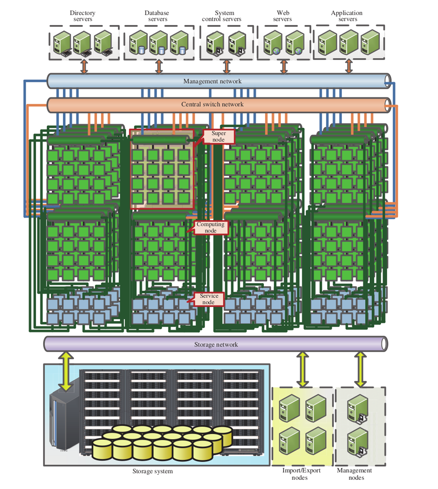
For situations where the budget does not allow for such an elaborate and highly customized system, or where the specific tasks do not warrant such an approach, there always remains the "Beowulf" approach. A Beowulf cluster is a term used to refer to a distributed computing system constructed out of common computer systems. These can be Intel or AMD-based x86 systems, with ARM-based processors now becoming popular.
It's generally helpful to have each node in a cluster to be roughly identical to the other nodes. Although it's possible to have an asymmetric cluster, management and job scheduling becomes much easier when one can make broad assumptions about each node.
At the very least, one would want to match the processor architecture, with a base level of CPU extensions, such as SSE2/3 and perhaps AVX and kin, common across all nodes. Doing this would allow one to use the same compiled binary across the nodes, along with the same algorithms, massively simplifying the deployment of jobs and the maintenance of the code base.
For the network between the nodes, Ethernet is a very popular option, delivering communication times measured in tens to hundreds of microseconds, while costing only a fraction of faster options. Usually each node would be connected to a single Ethernet network, as in this graphic:
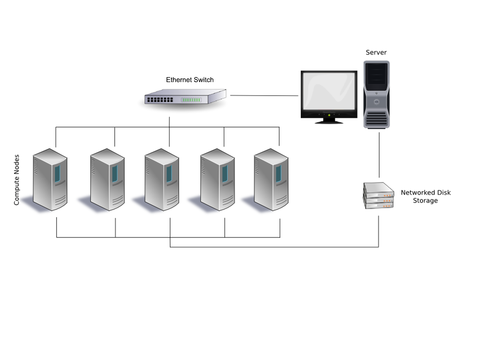
There is also the option to add a second or even third Ethernet link to each or specific nodes to give them access to files, I/O, and other resources, without having to compete with bandwidth on the primary network layer. For very large clusters, one could consider an approach such as that used with the Sunway TaihuLight and many other supercomputers: splitting nodes up into supernodes, each with their own inter-node network. This would allow one to optimize traffic on the network by limiting it to only associated nodes.
An example of such an optimized Beowulf cluster would look like this:
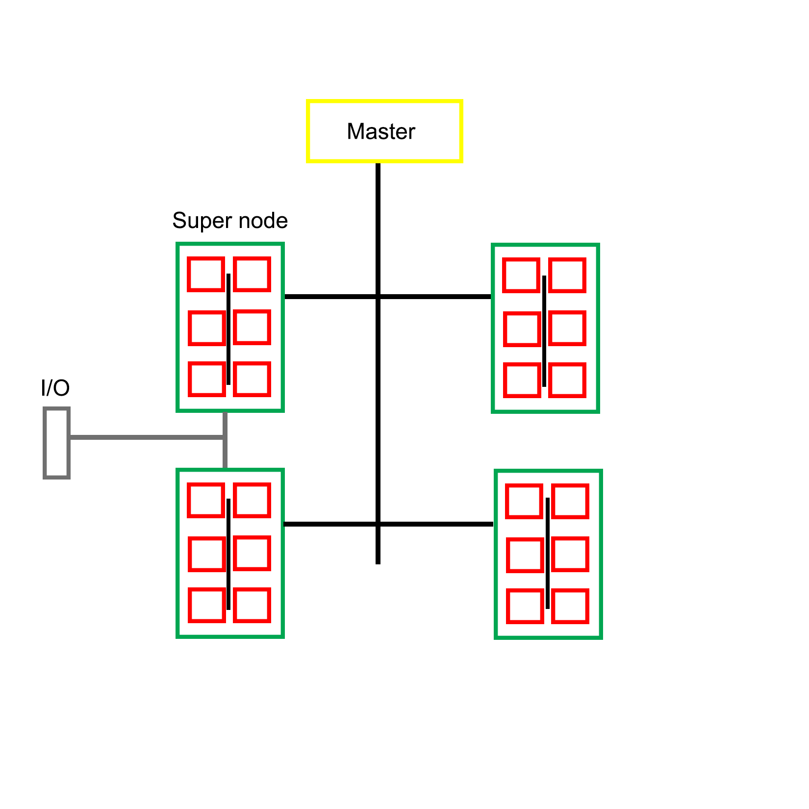
Clearly there is a wide range of possible configurations with MPI-based clusters, utilizing custom, off-the-shelf, or a combination of both types of hardware. The intended purpose of the cluster often determines the most optimal layout for a specific cluster, such as running simulations, or the processing of large datasets. Each type of job presents its own set of limitations and requirements, which is also reflected in the software implementation.
For the remainder of this chapter, we will focus on Open MPI. In order to get a working development environment for Open MPI, one will have to install its headers and library files, along with its supporting tools and binaries.
On Linux and BSD distributions with a package management system, it's quite easy: simply install the Open MPI package and everything should be set up and configured, ready to be used. Consult the manual for one's specific distribution, to see how to search for and install specific packages.
On Debian-based distributions, one would use:
$ sudo apt-get install openmpi-bin openmpi-doc libopenmpi-dev
The preceding command would install the Open MPI binaries, documentation, and development headers. The last two packages can be omitted on compute nodes.
On Windows things get slightly complex, mostly because of the dominating presence of Visual C++ and the accompanying compiler toolchain. If one wishes to use the same development environment as on Linux or BSD, using MinGW, one has to take some additional steps.
The easiest to use and most up to date MinGW environment is MSYS2, which provides a Bash shell along with most of the tools one would be familiar with under Linux and BSD. It also features the Pacman package manager, as known from the Linux Arch distribution. Using this, it's easy to install the requisite packages for Open MPI development.
After installing the MSYS2 environment from https://msys2.github.io/, install the MinGW toolchain:
$ pacman -S base-devel mingw-w64-x86_64-toolchain
This assumes that the 64-bit version of MSYS2 was installed. For the 32-bit version, select i686 instead of x86_64. After installing these packages, we will have both MinGW and the basic development tools installed. In order to use them, start a new shell using the MinGW 64-bit postfix in the name, either via the shortcut in the start menu, or by using the executable file in the MSYS2 install folder.
With MinGW ready, it's time to install MS-MPI version 7.x. This is Microsoft's implementation of MPI and the easiest way to use MPI on Windows. It's an implementation of the MPI-2 specification and mostly compatible with the MPICH2 reference implementation. Since MS-MPI libraries are not compatible between versions, we use this specific version.
Though version 7 of MS-MPI has been archived, it can still be downloaded via the Microsoft Download Center at https://www.microsoft.com/en-us/download/details.aspx?id=49926.
MS-MPI version 7 comes with two installers, msmpisdk.msi and MSMpiSetup.exe. Both need to be installed. Afterwards, we should be able to open a new MSYS2 shell and find the following environment variable set up:
$ printenv | grep "WIN|MSMPI"
MSMPI_INC=D:DevMicrosoftSDKsMPIInclude
MSMPI_LIB32=D:DevMicrosoftSDKsMPILibx86
MSMPI_LIB64=D:DevMicrosoftSDKsMPILibx64
WINDIR=C:Windows
This output for the printenv command shows that the MS-MPI SDK and runtime was properly installed. Next, we need to convert the static library from the Visual C++ LIB format to the MinGW A format:
$ mkdir ~/msmpi
$ cd ~/msmpi
$ cp "$MSMPI_LIB64/msmpi.lib" .
$ cp "$WINDIR/system32/msmpi.dll" .
$ gendef msmpi.dll
$ dlltool -d msmpi.def -D msmpi.dll -l libmsmpi.a
$ cp libmsmpi.a /mingw64/lib/.
We first copy the original LIB file into a new temporary folder in our home folder, along with the runtime DLL. Next, we use the gendef tool on the DLL in order to create the definitions which we will need in order to convert it to a new format.
This last step is done with dlltool, which takes the definitions file along with the DLL and outputs a static library file which is compatible with MinGW. This file we then copy to a location where MinGW can find it later when linking.
Next, we need to copy the MPI header:
$ cp "$MSMPI_INC/mpi.h" .
After copying this header file, we must open it and locate the section that starts with:
typedef __int64 MPI_Aint
Immediately above that line, we need to add the following line:
#include <stdint.h>
This include adds the definition for __int64, which we will need for the code to compile correctly.
Finally, copy the header file to the MinGW include folder:
$ cp mpi.h /mingw64/include
With this we have the libraries and headers all in place for MPI development with MinGW. allowing us to compile and run the earlier Hello World example, and continue with the rest of this chapter.
In order to distribute MPI jobs across the nodes in a cluster, one has to either specify these nodes as a parameter to the mpirun/mpiexec command or make use of a host file. This host file contains the names of the nodes on the network which will be available for a run, along with the number of available slots on the host.
A prerequisite for running MPI applications on a remote node is that the MPI runtime is installed on that node, and that password-less access has been configured for that node. This means that so long as the master node has the SSH keys installed, it can log into each of these nodes in order to launch the MPI application on it.
After installing MPI on a node, the next step is to set up password-less SSH access for the master node. This requires the SSH server to be installed on the node (part of the ssh package on Debian-based distributions). After this we need to generate and install the SSH key.
One way to easily do this is by having a common user on the master node and other nodes, and using an NFS network share or similar to mount the user folder on the master node on the compute nodes. This way all nodes would have the same SSH key and known hosts file. One disadvantage of this approach is the lack of security. For an internet-connected cluster, this would not be a very good approach.
It is, however, a definitely good idea to run the job on each node as the same user to prevent any possible permission issues, especially when using files and other resources. With the common user account created on each node, and with the SSH key generated, we can transfer the public key to the node using the following command:
$ ssh-copy-id mpiuser@node1
Alternatively, we can copy the public key into the authorized_keys file on the node system while we are setting it up. If creating and configuring a large number of nodes, it would make sense to use an image to copy onto each node's system drive, use a setup script, or possibly boot from an image through PXE boot.
With this step completed, the master node can now log into each compute node in order to run jobs.
As mentioned earlier, in order to run a job on other nodes, we need to specify these nodes. The easiest way to do this is to create a file containing the names of the compute nodes we wish to use, along with optional parameters.
To allow us to use names for the nodes instead of IP addresses, we have to modify the operating system's host file first: for example, /etc/hosts on Linux:
192.168.0.1 master
192.168.0.2 node0
192.168.0.3 node1
Next we create a new file which will be the host file for use with MPI:
master
node0
node1
With this configuration, a job would be executed on both compute nodes, as well as the master node. We can take the master node out of this file to prevent this.
Without any optional parameter provided, the MPI runtime will use all available processors on the node. If it is desirable, we can limit this number:
node0 slots=2
node1 slots=4
Assuming that both nodes are quad-core CPUs, this would mean that only half the cores on node0 would be used, and all of them on node1.
Running an MPI job across multiple MPI nodes is basically the same as executing it only locally, as in the example earlier in this chapter:
$ mpirun --hostfile my_hostfile hello_mpi_world
This command would tell the MPI launcher to use a host file called my_hostfile and run a copy of the specified MPI application on each processor of each node found in that host file.
In addition to using a manual command and host files to create and start jobs on specific nodes, there are also cluster scheduler applications. These generally involve the running of a daemon process on each node as well as the master node. Using the provided tools, one can then manage resources and jobs, scheduling allocation and keeping track of job status.
One of the most popular cluster management scheduler's is SLURM, which short for Simple Linux Utility for Resource management (though now renamed to Slurm Workload Manager with the website at https://slurm.schedmd.com/). It is commonly used by supercomputers as well as many computer clusters. Its primary functions consist out of:
The setting up of a cluster scheduler is not required for a basic cluster operation, but can be very useful for larger clusters, when running multiple jobs simultaneously, or when having multiple users of the cluster wishing to run their own job.
At this point, we have a functional MPI cluster, which can be used to execute MPI-based applications (and others, as well) in a parallel fashion. While for some tasks it might be okay to just send dozens or hundreds of processes on their merry way and wait for them to finish, very often it is crucial that these parallel processes are able to communicate with each other.
This is where the true meaning of MPI (being "Message Passing Interface") comes into play. Within the hierarchy created by an MPI job, processes can communicate and share data in a variety of ways. Most fundamentally, they can share and receive messages.
An MPI message has the following properties:
The sender and receiver should be fairly obvious. The message tag is a numeric ID which the sender can set and which the receiver can use to filter messages, to, for example, allow for the prioritizing of specific messages. The data type determines the type of information contained in the message.
The send and receive functions look like this:
int MPI_Send(
void* data,
int count,
MPI_Datatype datatype,
int destination,
int tag,
MPI_Comm communicator)
int MPI_Recv(
void* data,
int count,
MPI_Datatype datatype,
int source,
int tag,
MPI_Comm communicator,
MPI_Status* status)
An interesting thing to note here is that the count parameter in the send function indicates the number of elements that the function will be sending, whereas the same parameter in the receive function indicates the maximum number of elements that this thread will accept.
The communicator refers to the MPI communicator instance being used, and the receive function contains a final parameter which can be used to check the status of the MPI message.
MPI defines a number of basic types, which one can use directly:
|
MPI datatype |
C equivalent |
|
MPI_SHORT |
short int |
|
MPI_INT |
int |
|
MPI_LONG |
long int |
|
MPI_LONG_LONG |
long long int |
|
MPI_UNSIGNED_CHAR |
unsigned char |
|
MPI_UNSIGNED_SHORT |
unsigned short int |
|
MPI_UNSIGNED |
unsigned int |
|
MPI_UNSIGNED_LONG |
unsigned long int |
|
MPI_UNSIGNED_LONG_LONG |
unsigned long long int |
|
MPI_FLOAT |
float |
|
MPI_DOUBLE |
double |
|
MPI_LONG_DOUBLE |
long double |
|
MPI_BYTE |
char |
MPI guarantees that when using these types, the receiving side will always get the message data in the format it expects, regardless of endianness and other platform-related issues.
In addition to these basic formats, one can also create new MPI data types. These use a number of MPI functions, including MPI_Type_create_struct:
int MPI_Type_create_struct(
int count,
int array_of_blocklengths[],
const MPI_Aint array_of_displacements[],
const MPI_Datatype array_of_types[],
MPI_Datatype *newtype)
With this function, one can create an MPI type that contains a struct, to be passed just like a basic MPI data type:
#include <cstdio>
#include <cstdlib>
#include <mpi.h>
#include <cstddef>
struct car {
int shifts;
int topSpeed;
};
int main(int argc, char **argv) {
const int tag = 13;
int size, rank;
MPI_Init(&argc, &argv);
MPI_Comm_size(MPI_COMM_WORLD, &size);
if (size < 2) {
fprintf(stderr,"Requires at least two processes.n");
MPI_Abort(MPI_COMM_WORLD, 1);
}
const int nitems = 2;
int blocklengths[2] = {1,1};
MPI_Datatype types[2] = {MPI_INT, MPI_INT};
MPI_Datatype mpi_car_type;
MPI_Aint offsets[2];
offsets[0] = offsetof(car, shifts);
offsets[1] = offsetof(car, topSpeed);
MPI_Type_create_struct(nitems, blocklengths, offsets, types, &mpi_car_type);
MPI_Type_commit(&mpi_car_type);
MPI_Comm_rank(MPI_COMM_WORLD, &rank);
if (rank == 0) {
car send;
send.shifts = 4;
send.topSpeed = 100;
const int dest = 1;
MPI_Send(&send, 1, mpi_car_type, dest, tag, MPI_COMM_WORLD);
printf("Rank %d: sent structure carn", rank);
}
if (rank == 1) {
MPI_Status status;
const int src = 0;
car recv;
MPI_Recv(&recv, 1, mpi_car_type, src, tag, MPI_COMM_WORLD, &status);
printf("Rank %d: Received: shifts = %d topSpeed = %dn", rank, recv.shifts, recv.topSpeed);
}
MPI_Type_free(&mpi_car_type);
MPI_Finalize();
return 0;
}
Here we see how a new MPI data type called mpi_car_type is defined and used to message between two processes. To create a struct type like this, we need to define the number of items in the struct, the number of elements in each block, their byte displacement, and their basic MPI types.
A simple example of MPI communication is the sending of a single value from one process to another. In order to do this, one needs to use the following listed code and run the compiled binary to start at least two processes. It does not matter whether these processes run locally or on two compute nodes.
The following code was gratefully borrowed from http://mpitutorial.com/tutorials/mpi-hello-world/:
#include <mpi.h>
#include <stdio.h>
#include <stdlib.h>
int main(int argc, char** argv) {
// Initialize the MPI environment.
MPI_Init(NULL, NULL);
// Find out rank, size.
int world_rank;
MPI_Comm_rank(MPI_COMM_WORLD, &world_rank);
int world_size;
MPI_Comm_size(MPI_COMM_WORLD, &world_size);
// We are assuming at least 2 processes for this task.
if (world_size < 2) {
fprintf(stderr, "World size must be greater than 1 for %s.n", argv[0]);
MPI_Abort(MPI_COMM_WORLD, 1);
}
int number;
if (world_rank == 0) {
// If we are rank 0, set the number to -1 and send it to process 1.
number = -1;
MPI_Send(&number, 1, MPI_INT, 1, 0, MPI_COMM_WORLD);
}
else if (world_rank == 1) {
MPI_Recv(&number, 1, MPI_INT, 0, 0,
MPI_COMM_WORLD,
MPI_STATUS_IGNORE);
printf("Process 1 received number %d from process 0.n", number);
}
MPI_Finalize();
}
There isn't a lot to this code. We work through the usual MPI initialization, followed by a check to ensure that our world size is at least two processes large.
The process with rank 0 will then send an MPI message of data type MPI_INT and value -1. The process with rank 1 will wait to receive this message. The receiving process specifies for MPI_Status MPI_STATUS_IGNORE to indicate that the process will not be checking the status of the message. This is a useful optimization technique.
Finally, the expected output is the following:
$ mpirun -n 2 ./send_recv_demo
Process 1 received number -1 from process 0
Here we start the compiled demo code with a total of two processes. The output shows that the second process received the MPI message from the first process, with the correct value.
For advanced MPI communication, one would use the MPI_Status field to obtain more information about a message. One can use MPI_Probe to discover a message's size before accepting it with MPI_Recv. This can be useful for situations where it is not known beforehand what the size of a message will be.
Broadcasting a message means that all processes in the world will receive it. This simplifies the broadcast function relative to the send function:
int MPI_Bcast(
void *buffer,
int count,
MPI_Datatype datatype,
int root,
MPI_Comm comm)
The receiving processes would simply use a normal MPI_Recv function. All that the broadcast function does is optimize the sending of many messages using an algorithm that uses multiple network links simultaneously, instead of just one.
Scattering is very similar to broadcasting a message, with one very important distinction: instead of sending the same data in each message, instead it sends a different part of an array to each recipient. Its function definition looks as follows:
int MPI_Scatter(
void* send_data,
int send_count,
MPI_Datatype send_datatype,
void* recv_data,
int recv_count,
MPI_Datatype recv_datatype,
int root,
MPI_Comm communicator)
Each receiving process will get the same data type, but we can specify how many items will be sent to each process (send_count). This function is used on both the sending and receiving side, with the latter only having to define the last set of parameters relating to receiving data, with the world rank of the root process and the relevant communicator being provided.
Gathering is the inverse of scattering. Here multiple processes will send data that ends up at a single process, with this data sorted by the rank of the process which sent it. Its function definition looks as follows:
int MPI_Gather(
void* send_data,
int send_count,
MPI_Datatype send_datatype,
void* recv_data,
int recv_count,
MPI_Datatype recv_datatype,
int root,
MPI_Comm communicator)
One may notice that this function looks very similar to the scatter function. This is because it works basically the same way, only this time around the sending nodes have to all fill in the parameters related to sending the data, while the receiving process has to fill in the parameters related to receiving data.
It is important to note here that the recv_count parameter relates to the amount of data received from each sending process, not the size in total.
There exist further specializations of these two basic functions, but these will not be covered here.
One might think that it would be easiest to use MPI to allocate one instance of the MPI application to a single CPU core on each cluster node, and this would be true. It would, however, not be the fastest solution.
Although for communication between processes across a network MPI is likely the best choice in this context, within a single system (single or multi-CPU system) using multithreading makes a lot of sense.
The main reason for this is simply that communication between threads is significantly faster than inter-process communication, especially when using a generalized communication layer such as MPI.
One could write an application that uses MPI to communicate across the cluster's network, whereby one allocates one instance of the application to each MPI node. The application itself would detect the number of CPU cores on that system, and create one thread for each core. Hybrid MPI, as it's often called, is therefore commonly used, for the advantages it provides:
Implementing this can be done the way we have seen in previous chapters, by using the multithreading features found in C++11 and successive versions. The other option is to use OpenMP, as we saw at the very beginning of this chapter.
The obvious advantage of using OpenMP is that it takes very little effort from the developer's side. If all that one needs is to get more instances of the same routine running, all it takes is are the small modifications to mark the code to be used for the worker threads.
For example:
#include <stdio.h>
#include <mpi.h>
#include <omp.h>
int main(int argc, char *argv[]) {
int numprocs, rank, len;
char procname[MPI_MAX_PROCESSOR_NAME];
int tnum = 0, tc = 1;
MPI_Init(&argc, &argv);
MPI_Comm_size(MPI_COMM_WORLD, &numprocs);
MPI_Comm_rank(MPI_COMM_WORLD, &rank);
MPI_Get_processor_name(procname, &len);
#pragma omp parallel default(shared) private(tnum, tc) {
np = omp_get_num_threads();
tnum = omp_get_thread_num();
printf("Thread %d out of %d from process %d out of %d on %sn",
tnum, tc, rank, numprocs, procname);
}
MPI_Finalize();
}
The above code combines an OpenMP application with MPI. To compile it we would run for example:
$ mpicc -openmp hellohybrid.c -o hellohybrid
Next, to run the application, we would use mpirun or equivalent:
$ export OMP_NUM_THREADS=8
$ mpirun -np 2 --hostfile my_hostfile -x OMP_NUM_THREADS ./hellohybrid
The mpirun command would run two MPI processes using the hellohybrid binary, passing the environment variable we exported with the -x flag to each new process. The value contained in that variable will then be used by the OpenMP runtime to create that number of threads.
Assuming we have at least two MPI nodes in our MPI host file, we would end up with two MPI processes across two nodes, each of which running eight threads, which would fit a quad-core CPU with Hyper-Threading or an octo-core CPU.
When writing MPI-based applications and executing them on either a multi-core CPU or cluster, the issues one may encounter are very much the same as those we already came across with the multithreaded code in the preceding chapters.
However, an additional worry with MPI is that one relies on the availability of network resources. Since a send buffer used for an MPI_Send call cannot be reclaimed until the network stack can process the buffer, and this call is a blocking type, sending lots of small messages can lead to one process waiting for another, which in turn is waiting for a call to complete.
This type of deadlock should be kept in mind when designing the messaging structure of an MPI application. One can, for example, ensure that there are no send calls building up on one side, which would lead to such a scenario. Providing feedback messages on, queue depth and similar could be used to the ease pressure.
MPI also contains a synchronization mechanism using a so-called barrier. This is meant to be used between MPI processes to allow them to synchronize on for example a task. Using an MPI barrier (MPI_Barrier) call is similarly problematic as a mutex in that if an MPI process does not manage to get synchronized, everything will hang at this point.
In this chapter, we looked in some detail at the MPI standard, along with a number of its implementations, specifically Open MPI, and we looked at how to set up a cluster. We also saw how to use OpenMP to easily add multithreading to existing codes.
At this point, the reader should be capable of setting up a basic Beowulf or similar cluster, configuring it for MPI, and running basic MPI applications on it. How to communicate between MPI processes and how to define custom data types should be known. In addition, the reader will be aware of the potential pitfalls when programming for MPI.
In the next chapter, we will take all our knowledge of the preceding chapters and see how we can combine it in the final chapter, as we look at general-purpose computing on videocards (GPGPU).
A fairly recent development has been to use video cards (GPUs) for general purpose computing (GPGPU). Using frameworks such as CUDA and OpenCL, it is possible to speed up, for example, the processing of large datasets in parallel in medical, military, and scientific applications. In this chapter, we will look at how this is done with C++ and OpenCL, and how to integrate such a feature into a multithreaded application in C++.
Topics in this chapter include:
In Chapter 16, Multithreading with Distributed Computing, we looked at running the same task across a number of compute nodes in a cluster system. The main goal of such a setup is to process data in a highly parallel fashion, theoretically speeding up said processing relative to a single system with fewer CPU cores.
GPGPU (General Purpose Computing on Graphics Processing Units) is in some ways similar to this, but with one major difference: while a compute cluster with only regular CPUs is good at scalar tasks--meaning performing one task on one single set of data (SISD)--GPUs are vector processors that excel at SIMD (Single Input, Multiple Data) tasks.
Essentially, this means that one can send a large dataset to a GPU, along with a single task description, and the GPU will proceed to execute that same task on parts of that data in parallel on its hundreds or thousands of cores. One can thus regard a GPU as a very specialized kind of cluster:
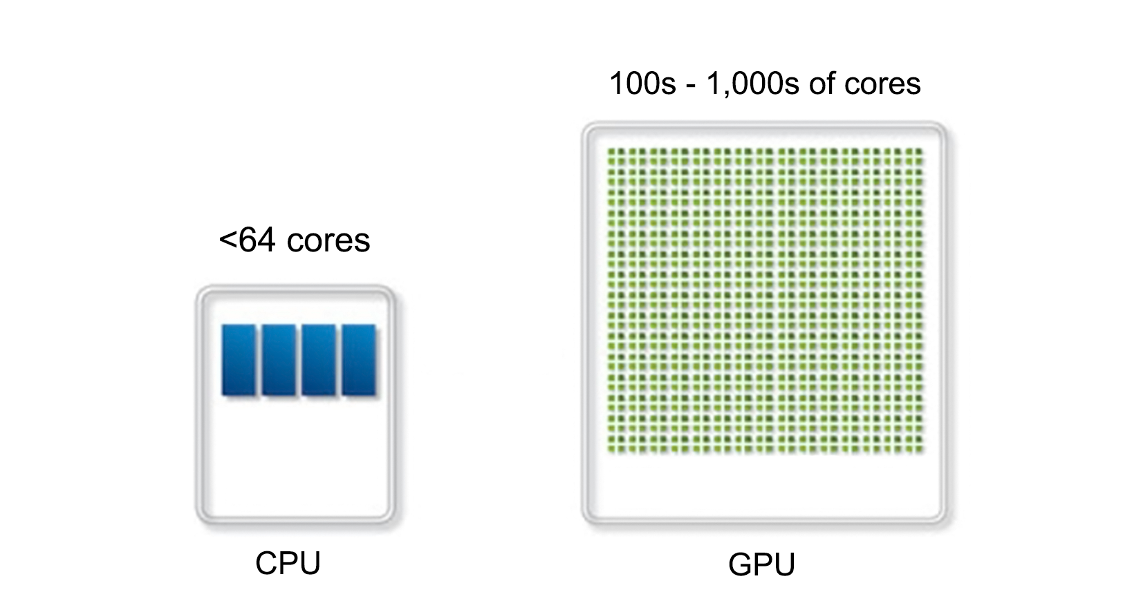
When the concept of GPGPU was first coined (around 2001), the most common way to write GPGPU programs was using GLSL (OpenGL Shading Language) and similar shader languages. Since these shader languages were already aimed at the processing of SIMD tasks (image and scene data), adapting them for more generic tasks was fairly straightforward.
Since that time, a number of more specialized implementations have appeared:
|
Name |
Since |
Owner |
Notes |
|
CUDA |
2006 |
NVidia |
This is proprietary and only runs on NVidia GPUs |
|
Close to Metal |
2006 |
ATi/AMD |
This was abandoned in favor of OpenCL |
|
DirectCompute |
2008 |
Microsoft |
This is released with DX11, runs on DX10 GPUs, and is limited to Windows platforms |
|
OpenCL |
2009 |
Khronos Group |
This is open standard and available across AMD, Intel, and NVidia GPUs on all mainstream platforms, as well as mobile platforms |
Of the various current GPGPU implementations, OpenCL is by far the most interesting GPGPU API due to the absence of limitations. It is available for virtually all mainstream GPUs and platforms, even enjoying support on select mobile platforms.
Another distinguishing feature of OpenCL is that it's not limited to just GPGPU either. As part of its name (Open Computing Language), it abstracts a system into the so-called compute devices, each with their own capabilities. GPGPU is the most common application, but this feature makes it fairly easy to test implementations on a CPU first, for easy debugging.
One possible disadvantage of OpenCL is that it employs a high level of abstraction for memory and hardware details, which can negatively affect performance, even as it increases the portability of the code.
In the rest of this chapter, we will focus on OpenCL.
Many programs incorporate OpenCL-based code in order to speed up operations. These include programs aimed at graphics processing, as well as 3D modelling and CAD, audio and video processing. Some examples are:
Further acceleration of certain operations is found in office applications including LibreOffice Calc and Microsoft Excel.
Perhaps more importantly, OpenCL is also commonly used for scientific computing and cryptography, including BOINC and GROMACS as well as many other libraries and programs.
Since the release of the OpenCL specification on December 8, 2008, there have so far been five updates, bringing it up to version 2.2. Important changes with these releases are mentioned next.
The first public release was released by Apple as part of the macOS X Snow Leopard release on August 28, 2009.
Together with this release, AMD announced that it would support OpenCL and retire its own Close to Metal (CtM) framework. NVidia, RapidMind, and IBM also added support for OpenCL to their own frameworks.
The OpenCL 1.1 specification was ratified by the Khronos Group on June 14, 2010. It adds additional functionality for parallel programming and performance, including the following:
The OpenCL 1.2 version was released on November 15, 2011. Its most significant features include the following:
The OpenCL2.0 version was released on November 18, 2013. This release has the following significant changes or additions:
The OpenCL 2.1 revision to the 2.0 standard was released on November 16, 2015. The most notable thing about this release was the introduction of the OpenCL C++ kernel language, such as how the OpenCL language originally was based on C with extensions, the C++ version is based on a subset of C++14, with backwards compatibility for the C kernel language.
Updates to the OpenCL API include the following:
Standard Portable Intermediate Representation (SPIR) and its successor, SPIR-V, are a way to provide device-independent binaries for use across OpenCL devices.
On May 16, 2017, what is now the current release of OpenCL was released. According to the Khronos Group, it includes the following changes:
Regardless of which platform and GPU you have, the most important part of doing OpenCL development is to obtain the OpenCL runtime for one's GPU from its manufacturer. Here, AMD, Intel, and NVidia all provide an SDK for all mainstream platforms. For NVidia, OpenCL support is included in the CUDA SDK.
Along with the GPU vendor's SDK, one can also find details on their website on which GPUs are supported by this SDK.
After installing the vendor's GPGPU SDK using the provided instructions, we still need to download the OpenCL headers. Unlike the shared library and runtime file provided by the vendor, these headers are generic and will work with any OpenCL implementation.
For Debian-based distributions, simply execute the following command line:
$ sudo apt-get install opencl-headers
For other distributions, the package may be called the same, or something different. Consult the manual for one's distribution on how to find out the package name.
After installing the SDK and OpenCL headers, we are ready to compile our first OpenCL applications.
On Windows, we can choose between developing with Visual Studio (Visual C++) or with the Windows port of GCC (MinGW). To stay consistent with the Linux version, we will be using MinGW along with MSYS2. This means that we'll have the same compiler toolchain and same Bash shell and utilities, along with the Pacman package manager.
After installing the vendor's GPGPU SDK, as described previously, simply execute the following command line in an MSYS2 shell in order to install the OpenCL headers:
$ pacman -S mingw64/mingw-w64-x86_64-opencl-headers
Or, execute the following command line when using the 32-bit version of MinGW:
mingw32/mingw-w64-i686-opencl-headers
With this, the OpenCL headers are in place. We now just have to make sure that the MinGW linker can find OpenCL library. With the NVidia CUDA SDK, you can use the CUDA_PATH environment variable for this, or browse the install location of the SDK and copy the appropriate OpenCL LIB file from there to the MinGW lib folder, making sure not to mix the 32-bit and 64-bit files.
With the shared library now also in place, we can compile the OpenCL applications.
Starting with OS X 10.7, an OpenCL runtime is provided with the OS. After installing XCode for the development headers and libraries, one can immediately start with OpenCL development.
A common example of a GPGPU application is one which calculates the Fast Fourier Transform (FFT). This algorithm is commonly used for audio processing and similar, allowing you to transform, for example, from the time domain to the frequency domain for analysis purposes.
What it does is apply a divide and conquer approach to a dataset, in order to calculate the DFT (Discrete Fourier Transform). It does this by splitting the input sequence into a fixed, small number of smaller subsequences, computing their DFT, and assembling these outputs in order to compose the final sequence.
This is fairly advanced mathematics, but suffice it to say that what makes it so ideal for GPGPU is that it's a highly-parallel algorithm, employing the subdivision of data in order to speed up the calculating of the DFT, as visualized in this graphic:
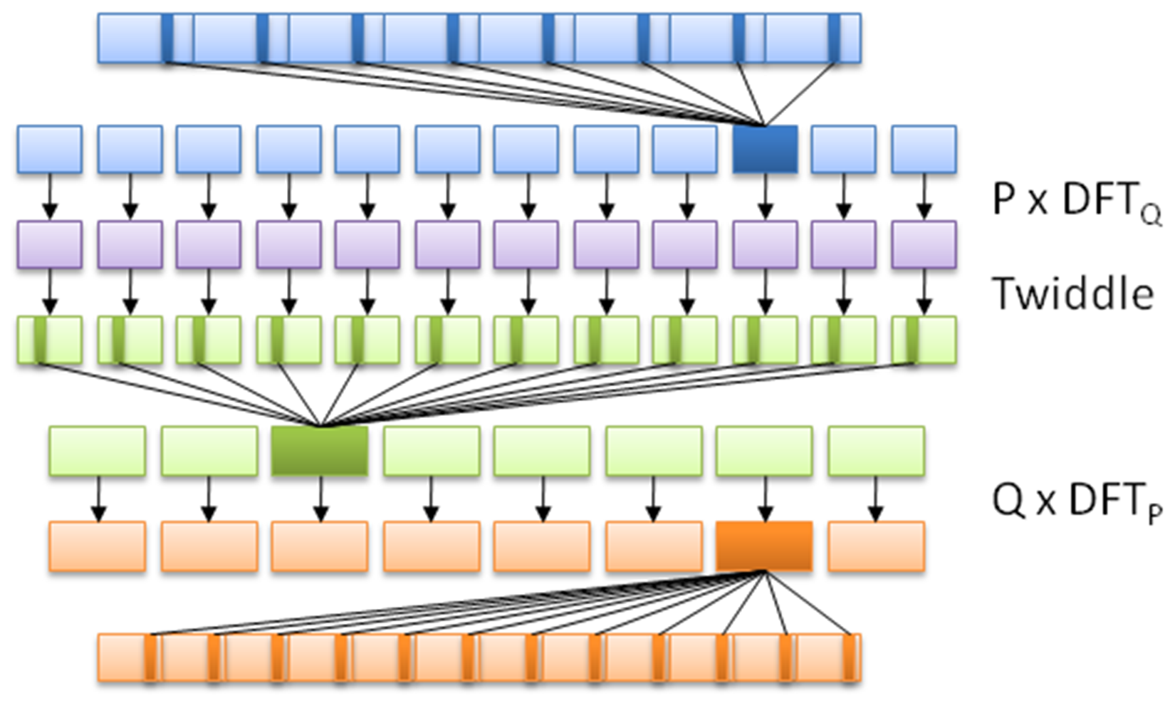
Each OpenCL application consists of at least two parts: the C++ code that sets up and configures the OpenCL instance, and the actual OpenCL code, also known as a kernel, such as this one based on the FFT demonstration example from Wikipedia:
// This kernel computes FFT of length 1024. // The 1024 length FFT is decomposed into calls to a radix 16 function, // another radix 16 function and then a radix 4 function
__kernel void fft1D_1024 (__global float2 *in, __global float2 *out, __local float *sMemx, __local float *sMemy) {
int tid = get_local_id(0);
int blockIdx = get_group_id(0) * 1024 + tid;
float2 data[16];
// starting index of data to/from global memory
in = in + blockIdx; out = out + blockIdx;
globalLoads(data, in, 64); // coalesced global reads
fftRadix16Pass(data); // in-place radix-16 pass
twiddleFactorMul(data, tid, 1024, 0);
// local shuffle using local memory
localShuffle(data, sMemx, sMemy, tid, (((tid & 15) * 65) + (tid >> 4)));
fftRadix16Pass(data); // in-place radix-16 pass
twiddleFactorMul(data, tid, 64, 4); // twiddle factor multiplication
localShuffle(data, sMemx, sMemy, tid, (((tid >> 4) * 64) + (tid & 15)));
// four radix-4 function calls
fftRadix4Pass(data); // radix-4 function number 1
fftRadix4Pass(data + 4); // radix-4 function number 2
fftRadix4Pass(data + 8); // radix-4 function number 3
fftRadix4Pass(data + 12); // radix-4 function number 4
// coalesced global writes
globalStores(data, out, 64);
}
This OpenCL kernel shows that, like the GLSL shader language, OpenCL's kernel language is essentially C with a number of extensions. Although one could use the OpenCL C++ kernel language, this one is only available since OpenCL 2.1 (2015), and as a result, support and examples for it are less common than the C kernel language.
Next is the C++ application, using which, we run the preceding OpenCL kernel:
#include <cstdio>
#include <ctime>
#include "CLopencl.h"
#define NUM_ENTRIES 1024
int main() { // (int argc, const char * argv[]) {
const char* KernelSource = "fft1D_1024_kernel_src.cl";
As we can see here, there's only one header we have to include in order to gain access to the OpenCL functions. We also specify the name of the file that contains the source for our OpenCL kernel. Since each OpenCL device is likely a different architecture, the kernel is compiled for the target device when we load it:
const cl_uint num = 1;
clGetDeviceIDs(0, CL_DEVICE_TYPE_GPU, 0, 0, (cl_uint*) num); cl_device_id devices[1];
clGetDeviceIDs(0, CL_DEVICE_TYPE_GPU, num, devices, 0);
Next, we have to obtain a list of OpenCL devices we can use, filtering it by GPUs:
cl_context context = clCreateContextFromType(0, CL_DEVICE_TYPE_GPU,
0, 0, 0);
We then create an OpenCL context using the GPU devices we found. The context manages the resources on a range of devices:
clGetDeviceIDs(0, CL_DEVICE_TYPE_DEFAULT, 1, devices, 0);
cl_command_queue queue = clCreateCommandQueue(context, devices[0], 0, 0);
Finally, we will create the command queue that will contain the commands to be executed on the OpenCL devices:
cl_mem memobjs[] = { clCreateBuffer(context, CL_MEM_READ_ONLY | CL_MEM_COPY_HOST_PTR, sizeof(float) * 2 * NUM_ENTRIES, 0, 0),
clCreateBuffer(context, CL_MEM_READ_WRITE, sizeof(float) * 2 * NUM_ENTRIES, 0, 0) };
In order to communicate with devices, we need to allocate buffer objects that will contain the data we will copy to their memory. Here, we will allocate two buffers, one to read and one to write:
cl_program program = clCreateProgramWithSource(context, 1, (const char **)& KernelSource, 0, 0);
We have now got the data on the device, but still need to load the kernel on it. For this, we will create a kernel using the OpenCL kernel source we looked at earlier, using the filename we defined earlier:
clBuildProgram(program, 0, 0, 0, 0, 0);
Next, we will compile the source as follows:
cl_kernel kernel = clCreateKernel(program, "fft1D_1024", 0);
Finally, we will create the actual kernel from the binary we created:
size_t local_work_size[1] = { 256 };
clSetKernelArg(kernel, 0, sizeof(cl_mem), (void *) &memobjs[0]);
clSetKernelArg(kernel, 1, sizeof(cl_mem), (void *) &memobjs[1]);
clSetKernelArg(kernel, 2, sizeof(float) * (local_work_size[0] + 1) * 16, 0);
clSetKernelArg(kernel, 3, sizeof(float) * (local_work_size[0] + 1) * 16, 0);
In order to pass arguments to our kernel, we have to set them here. Here, we will add pointers to our buffers and dimensions of the work size as follows:
size_t global_work_size[1] = { 256 };
global_work_size[0] = NUM_ENTRIES;
local_work_size[0] = 64; // Nvidia: 192 or 256
clEnqueueNDRangeKernel(queue, kernel, 1, 0, global_work_size, local_work_size, 0, 0, 0);
Now we can set the work item dimensions and execute the kernel. Here, we will use a kernel execution method that allows us to define the size of the work group:
cl_mem C = clCreateBuffer(context, CL_MEM_WRITE_ONLY, (size), 0, &ret);
cl_int ret = clEnqueueReadBuffer(queue, memobjs[1], CL_TRUE, 0, sizeof(float) * 2 * NUM_ENTRIES, C, 0, 0, 0);
After executing the kernel, we wish to read back the resulting information. For this, we tell OpenCL to copy the assigned write buffer we passed as a kernel argument into a newly assigned buffer. We are now free to use the data in this buffer as we see fit.
However, in this example, we will not use the data:
clReleaseMemObject(memobjs[0]);
clReleaseMemObject(memobjs[1]); clReleaseCommandQueue(queue); clReleaseKernel(kernel); clReleaseProgram(program); clReleaseContext(context); free(C);
}
Finally, we free the resources we allocated and exit.
When using a CPU, one has to deal with a number of memory hierarchies, in the form of the main memory (slowest), to CPU caches (faster), and CPU registers (fastest). A GPU is much the same, in that, one has to deal with a memory hierarchy that can significantly impact the speed of one's applications.
Fastest on a GPU is also the register (or private) memory, of which we have quite a bit more than on the average CPU. After this, we get local memory, which is a memory shared by a number of processing elements. Slowest on the GPU itself is the memory data cache, also called texture memory. This is a memory on the card that is usually referred to as Video RAM (VRAM) and uses a high-bandwidth, but a relatively high-latency memory such as GDDR5.
The absolute slowest is using the host system's memory (system RAM), as this has to travel across the PCIe bus and through various other subsystems in order to transfer any data. Relative to on-device memory systems, host-device communication is best called 'glacial'.
For AMD, Nvidia, and similar dedicated GPU devices, the memory architecture can be visualized like this:
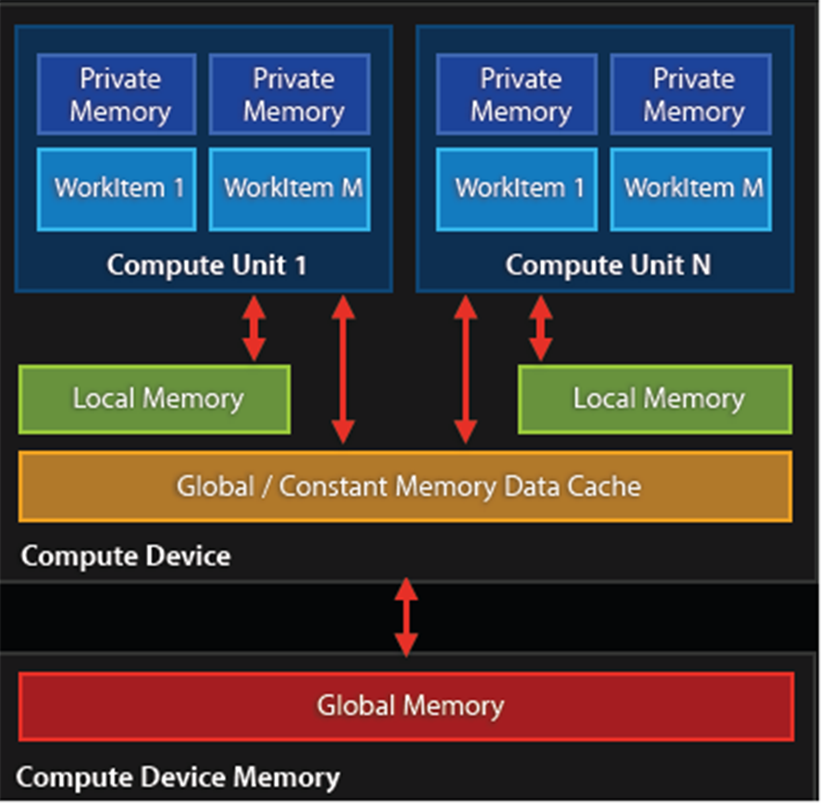
Because of this memory layout, it is advisable to transfer any data in large blocks, and to use asynchronous transfers if possible. Ideally, the kernel would run on the GPU core and have the data streamed to it to avoid any latencies.
Combining multithreaded code with GPGPU can be much easier than trying to manage a parallel application running on an MPI cluster. This is mostly due to the following workflow:
As this is an asynchronous process, one can treat this as a fire-and-forget operation, merely having a single thread dedicated to monitoring the process of the active kernels.
The biggest challenge in terms of multithreading and GPGPU applications lies not with the host-based application, but with the GPGPU kernel or shader program running on the GPU, as it has to coordinate memory management and processing between both local and distant processing units, determine which memory systems to use depending on the type of data without causing problems elsewhere in the processing.
This is a delicate process involving a lot of trial and error, profiling and optimizations. One memory copy optimization or use of an asynchronous operation instead of a synchronous one may cut processing time from many hours to just a couple. A good understanding of the memory systems is crucial to preventing data starvation and similar issues.
Since GPGPU is generally used to accelerate tasks of significant duration (minutes to hours, or longer), it is probably best regarded from a multithreading perspective as a common worker thread, albeit with a few important complications, mostly in the form of latency.
As we touched upon in the earlier section on GPU memory management, it is highly preferable to use the memory closest to the GPU's processing units first, as they are the fastest. Fastest here mostly means that they have less latency, meaning the time taken to request information from the memory and receiving the response.
The exact latency will differ per GPU, but as an example, for Nvidia's Kepler (Tesla K20) architecture, one can expect a latency of:
These measurements are all on the CPU itself. For the PCIe bus one would have to expect something on the order of multiple milliseconds per transfer once one starts to transfer multi-megabyte buffers. To fill for example the GPU's memory with a gigabyte-sized buffer could take a considerable amount of time.
For a simple round-trip over the PCIe bus one would measure the latency in microseconds, which for a GPU core running at 1+ GHz would seem like an eternity. This basically defines why communication between the host and GPU should be absolutely minimal and highly optimized.
A common mistake with GPGPU applications is reading the result buffer before the processing has finished. After transferring the buffer to the device and executing the kernel, one has to insert synchronization points to signal the host that it has finished processing. These generally should be implemented using asynchronous methods.
As we just covered in the section on latency, it's important to keep in mind the potentially very large delays between a request and response, depending on the memory sub-system or bus. Failure to do so may cause weird glitches, freezes and crashes, as well as data corruption and an application which will seemingly wait forever.
It is crucial to profile a GPGPU application to get a good idea of what the GPU utilization is, and whether the process flow is anywhere near being optimal.
The biggest challenge with GPGPU applications is that of debugging a kernel. CUDA comes with a simulator for this reason, which allows one to run and debug a kernel on a CPU. OpenCL allows one to run a kernel on a CPU without modification, although this may not get the exact same behavior (and bugs) as when run on a specific GPU device.
A slightly more advanced method involves the use of a dedicated debugger such as Nvidia's Nsight, which comes in versions both for Visual Studio (https://developer.nvidia.com/nvidia-nsight-visual-studio-edition) and Eclipse (https://developer.nvidia.com/nsight-eclipse-edition).
According to the marketing blurb on the Nsight website:
The following screenshot shows an active CUDA debug session:
A big advantage of such a debugger tool is that it allows one to monitor, profile and optimize one's GPGPU application by identifying bottlenecks and potential problems.
In this chapter, we looked at how to integrate GPGPU processing into a C++ application in the form of OpenCL. We also looked at the GPU memory hierarchy and how this impacts performance, especially in terms of host-device communication.
You should now be familiar with GPGPU implementations and concepts, along with how to create an OpenCL application, and how to compile and run it. How to avoid common mistakes should also be known.
As this is the final chapter of this book, it is hoped that all major questions have been answered, and that the preceding chapters, along with this one, have been informative and helpful in some fashion.
Moving on from this book, the reader may be interested in pursuing any of the topics covered in more detail, for which many resources are available both online and offline. The topic of multithreading and related areas is very large and touches upon many applications, from business to scientific, artistic and personal applications
The reader may want to set up a Beowulf cluster of tehir own, or focus on GPGPU, or combine the two. Maybe there is a complex application they have wanted to write for a while, or perhaps just have fun with programming.
In this chapter, we will cover the following recipes:
C++ got a lot of additions in C++11, C++14, and, most recently, C++17. By now, it is a completely different language compared to what it was just a decade ago. The C++ standard does not only standardize the language, as it needs to be understood by the compilers, but also the C++ standard template library (STL).
This book explains how to put the STL to the best use with a broad range of examples. But at first, this chapter will concentrate on the most important new language features. Mastering them will greatly help you write readable, maintainable, and expressive code a lot.
We will see how to access individual members of pairs, tuples, and structures comfortably with structured bindings and how to limit variable scopes with the new if and switch variable initialization capabilities. The syntactical ambiguities, which were introduced by C++11 with the new bracket initialization syntax, which looks the same for initializer lists, were fixed by new bracket initializer rules. The exact type of template class instances can now be deduced from the actual constructor arguments, and if different specializations of a template class will result in completely different code, this is now easily expressible with constexpr-if. The handling of variadic parameter packs in template functions became much easier in many cases with the new fold expressions. At last, it became more comfortable to define static globally accessible objects in header-only libraries with the new ability to declare inline variables, which was only possible for functions before.
Some of the examples in this chapter might be more interesting for implementers of libraries than for developers who implement applications. While we will have a look at such features for completeness reasons, it is not too critical to understand all the examples of this chapter immediately in order to understand the rest of this book.
C++17 comes with a new feature, which combines syntactic sugar and automatic type deduction: structured bindings. These help to assign values from pairs, tuples, and structs into individual variables. In other programming languages, this is also called unpacking.
Applying a structured binding in order to assign multiple variables from one bundled structure is always one step. Let's first see how it was done before C++17. Then, we can have a look at multiple examples that show how we can do it in C++17:
std::pair<int, int> divide_remainder(int dividend, int divisor);
Consider the following way of accessing the individual values of the resulting pair:
const auto result (divide_remainder(16, 3));
std::cout << "16 / 3 is "
<< result.first << " with a remainder of "
<< result.second << 'n';
Instead of doing it as shown in the preceding code snippet, we can now assign the individual values to individual variables with expressive names, which is much better to read:
auto [fraction, remainder] = divide_remainder(16, 3);
std::cout << "16 / 3 is "
<< fraction << " with a remainder of "
<< remainder << 'n';
std::tuple<std::string,
std::chrono::system_clock::time_point, unsigned>
stock_info(const std::string &name);
Assigning its result to individual variables looks just like in the example before:
const auto [name, valid_time, price] = stock_info("INTC");
struct employee {
unsigned id;
std::string name;
std::string role;
unsigned salary;
};
Now, we can access these members using structured bindings. We can even do that in a loop, assuming we have a whole vector of those:
int main()
{
std::vector<employee> employees {
/* Initialized from somewhere */};
for (const auto &[id, name, role, salary] : employees) {
std::cout << "Name: " << name
<< "Role: " << role
<< "Salary: " << salary << 'n';
}
}
Structured bindings are always applied with the same pattern:
auto [var1, var2, ...] = <pair, tuple, struct, or array expression>;
If we write too many or not enough variables between the square brackets, the compiler will error out, telling us about our mistake:
std::tuple<int, float, long> tup {1, 2.0, 3};
auto [a, b] = tup; // Does not work
This example obviously tries to stuff a tuple variable with three members into only two variables. The compiler immediately chokes on this and tells us about our mistake:
error: type 'std::tuple<int, float, long>' decomposes into 3 elements, but only 2 names were provided
auto [a, b] = tup;
A lot of fundamental data structures from the STL are immediately accessible using structured bindings without us having to change anything. Consider, for example, a loop that prints all the items of an std::map:
std::map<std::string, size_t> animal_population {
{"humans", 7000000000},
{"chickens", 17863376000},
{"camels", 24246291},
{"sheep", 1086881528},
/* … */
};
for (const auto &[species, count] : animal_population) {
std::cout << "There are " << count << " " << species
<< " on this planet.n";
}
This particular example works because when we iterate over an std::map container, we get the std::pair<const key_type, value_type> nodes on every iteration step. Exactly these nodes are unpacked using the structured bindings feature (key_type is the species string and value_type is the population count size_t) in order to access them individually in the loop body.
Before C++17, it was possible to achieve a similar effect using std::tie:
int remainder;
std::tie(std::ignore, remainder) = divide_remainder(16, 5);
std::cout << "16 % 5 is " << remainder << 'n';
This example shows how to unpack the resulting pair into two variables. The std::tie is less powerful than structured bindings in the sense that we have to define all the variables we want to bind to before. On the other hand, this example shows a strength of std::tie that structured bindings do not have: the value std::ignore acts as a dummy variable. The fraction part of the result is assigned to it, which leads to that value being dropped because we do not need it in that example.
Back in the past, the divide_remainder function could have been implemented in the following way, using output parameters:
bool divide_remainder(int dividend, int divisor,
int &fraction, int &remainder);
Accessing it would have looked like the following:
int fraction, remainder;
const bool success {divide_remainder(16, 3, fraction, remainder)};
if (success) {
std::cout << "16 / 3 is " << fraction << " with a remainder of "
<< remainder << 'n';
}
A lot of people will still prefer this over returning complex structures like pairs, tuples, and structs, arguing that this way the code would be faster, due to avoided intermediate copies of those values. This is not true any longer for modern compilers, which optimize intermediate copies away.
It is good style to limit the scope of variables as much as possible. Sometimes, however, one first needs to obtain some value, and only if it fits a certain condition, it can be processed further.
For this purpose, C++17 comes with if and switch statements with initializers.
In this recipe, we use the initializer syntax in both the supported contexts in order to see how they tidy up our code:
if (auto itr (character_map.find(c)); itr != character_map.end()) {
// *itr is valid. Do something with it.
} else {
// itr is the end-iterator. Don't dereference.
}
// itr is not available here at all
switch (char c (getchar()); c) {
case 'a': move_left(); break;
case 's': move_back(); break;
case 'w': move_fwd(); break;
case 'd': move_right(); break;
case 'q': quit_game(); break;
case '0'...'9': select_tool('0' - c); break;
default:
std::cout << "invalid input: " << c << 'n';
}
The if and switch statements with initializers are basically just syntax sugar. The following two samples are equivalent:
Before C++17:
{
auto var (init_value);
if (condition) {
// branch A. var is accessible
} else {
// branch B. var is accessible
}
// var is still accessible
}
Since C++17:
if (auto var (init_value); condition) {
// branch A. var is accessible
} else {
// branch B. var is accessible
}
// var is not accessible any longer
The same applies to switch statements:
Before C++17:
{
auto var (init_value);
switch (var) {
case 1: ...
case 2: ...
...
}
// var is still accessible
}
Since C++17:
switch (auto var (init_value); var) {
case 1: ...
case 2: ...
...
}
// var is not accessible any longer
This feature is very useful to keep the scope of a variable as short as necessary. Before C++17, this was only possible using extra braces around the code, as the pre-C++17 examples show. The short lifetimes reduce the number of variables in the scope, which keeps our code tidy and makes it easier to refactor.
Another interesting use case is the limited scope of critical sections. Consider the following example:
if (std::lock_guard<std::mutex> lg {my_mutex}; some_condition) {
// Do something
}
At first, an std::lock_guard is created. This is a class that accepts a mutex argument as a constructor argument. It locks the mutex in its constructor, and when it runs out of scope, it unlocks it again in its destructor. This way, it is impossible to forget to unlock the mutex. Before C++17, a pair of extra braces was needed in order to determine the scope where it unlocks again.
Yet another interesting use case is the scope of weak pointers. Consider the following:
if (auto shared_pointer (weak_pointer.lock()); shared_pointer != nullptr) {
// Yes, the shared object does still exist
} else {
// shared_pointer var is accessible, but a null pointer
}
// shared_pointer is not accessible any longer
This is another example where we would have a useless shared_pointer variable leaking into the current scope, although it has a potentially useless state outside the if conditional block or noisy extra brackets!
The if statements with initializers are especially useful when using legacy APIs with output parameters:
if (DWORD exit_code; GetExitCodeProcess(process_handle, &exit_code)) {
std::cout << "Exit code of process was: " << exit_code << 'n';
}
// No useless exit_code variable outside the if-conditional
GetExitCodeProcess is a Windows kernel API function. It returns the exit code for a given process handle but only if that handle is valid. After leaving this conditional block, the variable is useless, so we don't need it in any scope any longer.
Being able to initialize variables within if blocks is obviously very useful in a lot of situations and, especially, when dealing with legacy APIs that use output parameters.
C++11 came with the new brace initializer syntax {}. Its purpose was to allow for aggregate initialization, but also for usual constructor calling. Unfortunately, it was too easy to express the wrong thing when combining this syntax with the auto variable type. C++17 comes with an enhanced set of initializer rules. In this recipe, we will clarify how to correctly initialize variables with which syntax in C++17.
Variables are initialized in one step. Using the initializer syntax, there are two different situations:
// Three identical ways to initialize an int:
int x1 = 1;
int x2 {1};
int x3 (1);
std::vector<int> v1 {1, 2, 3}; // Vector with three ints: 1, 2, 3
std::vector<int> v2 = {1, 2, 3}; // same here
std::vector<int> v3 (10, 20); // Vector with 10 ints,
// each have value 20
auto v {1}; // v is int
auto w {1, 2}; // error: only single elements in direct
// auto initialization allowed! (this is new)
auto x = {1}; // x is std::initializer_list<int>
auto y = {1, 2}; // y is std::initializer_list<int>
auto z = {1, 2, 3.0}; // error: Cannot deduce element type
Without auto type deduction, there's not much to be surprised about in the brace {} operator, at least, when initializing regular types. When initializing containers such as std::vector, std::list, and so on, a brace initializer will match the std::initializer_list constructor of that container class. It does this in a greedy manner, which means that it is not possible to match non-aggregate constructors (non-aggregate constructors are usual constructors in contrast to the ones that accept an initializer list).
std::vector, for example, provides a specific non-aggregate constructor, which fills arbitrarily many items with the same value: std::vector<int> v (N, value). When writing std::vector<int> v {N, value}, the initializer_list constructor is chosen, which will initialize the vector with two items: N and value. This is a special pitfall one should know about.
One nice detail about the {} operator compared to constructor calling using normal () parentheses is that they do no implicit type conversions: int x (1.2); and int x = 1.2; will initialize x to value 1 by silently rounding down the floating point value and converting it to int. int x {1.2};, in contrast, will not compile because it wants to exactly match the constructor type.
The additional rule introduced in C++17 affects the initialization with auto type deduction--while C++11 would correctly make the type of the variable auto x {123}; an std::initializer_list<int> with only one element, this is seldom what we would want. C++17 would make the same variable an int.
Rule of thumb:
C++17 has made it harder to accidentally define an initializer list.
A lot of classes in C++ are usually specialized on types, which could be easily deduced from the variable types the user puts in their constructor calls. Nevertheless, before C++17, this was not a standardized feature. C++17 lets the compiler automatically deduce template types from constructor calls.
A very handy use case for this is constructing std::pair and std::tuple instances. These can be specialized and instantiated and specialized in one step:
std::pair my_pair (123, "abc"); // std::pair<int, const char*>
std::tuple my_tuple (123, 12.3, "abc"); // std::tuple<int, double,
// const char*>
Let’s define an example class where automatic template type deduction would be of value:
template <typename T1, typename T2, typename T3>
class my_wrapper {
T1 t1;
T2 t2;
T3 t3;
public:
explicit my_wrapper(T1 t1_, T2 t2_, T3 t3_)
: t1{t1_}, t2{t2_}, t3{t3_}
{}
/* … */
};
Okay, this is just another template class. We previously had to write the following in order to instantiate it:
my_wrapper<int, double, const char *> wrapper {123, 1.23, "abc"};
We can now just omit the template specialization part:
my_wrapper wrapper {123, 1.23, "abc"};
Before C++17, this was only possible by implementing a make function helper:
my_wrapper<T1, T2, T3> make_wrapper(T1 t1, T2 t2, T3 t3)
{
return {t1, t2, t3};
}
Using such helpers, it was possible to have a similar effect:
auto wrapper (make_wrapper(123, 1.23, "abc"));
What we just learned about was implicit template type deduction. In some cases, we cannot rely on implicit type deduction. Consider the following example class:
template <typename T>
struct sum {
T value;
template <typename ... Ts>
sum(Ts&& ... values) : value{(values + ...)} {}
};
This struct, sum, accepts an arbitrary number of parameters and adds them together using a fold expression (have a look at the fold expression recipe a little later in this chapter to get more details on fold expressions). The resulting sum is saved in the member variable value. Now the question is, what type is T? If we don't want to specify it explicitly, it surely needs to depend on the types of the values provided in the constructor. If we provide string instances, it needs to be std::string. If we provide integers, it needs to be int. If we provide integers, floats, and doubles, the compiler needs to figure out which type fits all the values without information loss. In order to achieve that, we provide an explicit deduction guide:
template <typename ... Ts>
sum(Ts&& ... ts) -> sum<std::common_type_t<Ts...>>;
This deduction guide tells the compiler to use the std::common_type_t trait, which is able to find out which common type fits all the values. Let's see how to use it:
sum s {1u, 2.0, 3, 4.0f};
sum string_sum {std::string{"abc"}, "def"};
std::cout << s.value << 'n'
<< string_sum.value << 'n';
In the first line we instantiate a sum object with constructor arguments of type unsigned, double, int, and float. The std::common_type_t returns double as the common type, so we get a sum<double> instance. In the second line, we provide an std::string instance and a C-style string. Following our deduction guide, the compiler constructs an instance of type sum<std::string>.
When running this code, it will print 10 as the numeric sum and abcdef as the string sum.
In templated code, it is often necessary to do certain things differently, depending on the type the template is specialized for. C++17 comes with constexpr-if expressions, which simplify the code in such situations a lot.
In this recipe, we'll implement a little helper template class. It can deal with different template type specializations because it is able to select completely different code in some passages, depending on what type we specialize it for:
template <typename T>
class addable
{
T val;
public:
addable(T v) : val{v} {}
template <typename U>
T add(U x) const {
return val + x;
}
};
template <typename U>
T add(U x)
{
auto copy (val); // Get a copy of the vector member
for (auto &n : copy) {
n += x;
}
return copy;
}
template <typename U>
T add(U x) const {
if constexpr (std::is_same_v<T, std::vector<U>>) {
auto copy (val);
for (auto &n : copy) {
n += x;
}
return copy;
} else {
return val + x;
}
}
addable<int>{1}.add(2); // is 3
addable<float>{1.0}.add(2); // is 3.0
addable<std::string>{"aa"}.add("bb"); // is "aabb"
std::vector<int> v {1, 2, 3};
addable<std::vector<int>>{v}.add(10);
// is std::vector<int>{11, 12, 13}
std::vector<std::string> sv {"a", "b", "c"};
addable<std::vector<std::string>>{sv}.add(std::string{"z"});
// is {"az", "bz", "cz"}
The new constexpr-if works exactly like usual if-else constructs. The difference is that the condition that it tests has to be evaluated at compile time. All runtime code that the compiler creates from our program will not contain any branch instructions from constexpr-if conditionals. One could also put it that it works in a similar manner to preprocessor #if and #else text substitution macros, but for those, the code would not even have to be syntactically well-formed. All the branches of a constexpr-if construct need to be syntactically well-formed, but the branches that are not taken do not need to be semantically valid.
In order to distinguish whether the code should add the value x to a vector or not, we use the type trait std::is_same. An expression std::is_same<A, B>::value evaluates to the Boolean value true if A and B are of the same type. The condition used in our recipe is std::is_same<T, std::vector<U>>::value, which evaluates to true if the user specialized the class on T = std::vector<X> and tries to call add with a parameter of type U = X.
There can, of course, be multiple conditions in one constexpr-if-else block (note that a and b have to depend on template parameters and not only on compile-time constants):
if constexpr (a) {
// do something
} else if constexpr (b) {
// do something else
} else {
// do something completely different
}
With C++17, a lot of meta programming situations are much easier to express and to read.
In order to relate how much constexpr-if constructs are an improvement to C++, we can have a look at how the same thing could have been implemented before C++17:
template <typename T>
class addable
{
T val;
public:
addable(T v) : val{v} {}
template <typename U>
std::enable_if_t<!std::is_same<T, std::vector<U>>::value, T>
add(U x) const { return val + x; }
template <typename U>
std::enable_if_t<std::is_same<T, std::vector<U>>::value,
std::vector<U>>
add(U x) const {
auto copy (val);
for (auto &n : copy) {
n += x;
}
return copy;
}
};
Without using constexpr-if, this class works for all different types we wished for, but it looks super complicated. How does it work?
The implementations alone of the two different add functions look simple. It's their return type declaration, which makes them look complicated, and which contains a trick--an expression such as std::enable_if_t<condition, type> evaluates to type if condition is true. Otherwise, the std::enable_if_t expression does not evaluate to anything. That would normally considered an error, but we will see why it is not.
For the second add function, the same condition is used in an inverted manner. This way, it can only be true at the same time for one of the two implementations.
When the compiler sees different template functions with the same name and has to choose one of them, an important principle comes into play: SFINAE, which stands for Substitution Failure is not an Error. In this case, this means that the compiler does not error out if the return value of one of those functions cannot be deduced from an erroneous template expression (which std::enable_if is, in case its condition evaluates to false). It will simply look further and try the other function implementation. That is the trick; that is how this works.
What a hassle. It is nice to see that this became so much easier with C++17.
While it was always possible in C++ to declare individual functions inline, C++17 additionally allows us to declare variables inline. This makes it much easier to implement header-only libraries, which was previously only possible using workarounds.
In this recipe, we create an example class that could suit as a member of a typical header-only library. The target is to give it a static member and instantiate it in a globally available manner using the inline keyword, which would not be possible like this before C++17:
// foo_lib.hpp
class process_monitor {
public:
static const std::string standard_string
{"some static globally available string"};
};
process_monitor global_process_monitor;
// foo_lib.hpp
class process_monitor {
public:
static const inline std::string standard_string
{"some static globally available string"};
};
inline process_monitor global_process_monitor;
Voila, that's it!
C++ programs do often consist of multiple C++ source files (these do have .cpp or .cc suffices). These are individually compiled to modules/object files (which usually have .o suffices). Linking all the modules/object files together into a single executable or shared/static library is then the last step.
At the link stage, it is considered an error if the linker can find the definition of one specific symbol multiple times. Let's say, for example, we have a function with a signature such as int foo();. If two modules define the same function, which is the right one? The linker can't just roll the dice. Well, it could, but that's most likely not what any programmer would ever want to happen.
The traditional way to provide globally available functions is to declare them in the header files, which will be included by any C++ module that needs to call them. The definition of every of those functions will be then put once into separate module files. These are then linked together with the modules that desire to use these functions. This is also called the One Definition Rule (ODR). Check out the following illustration for better understanding:
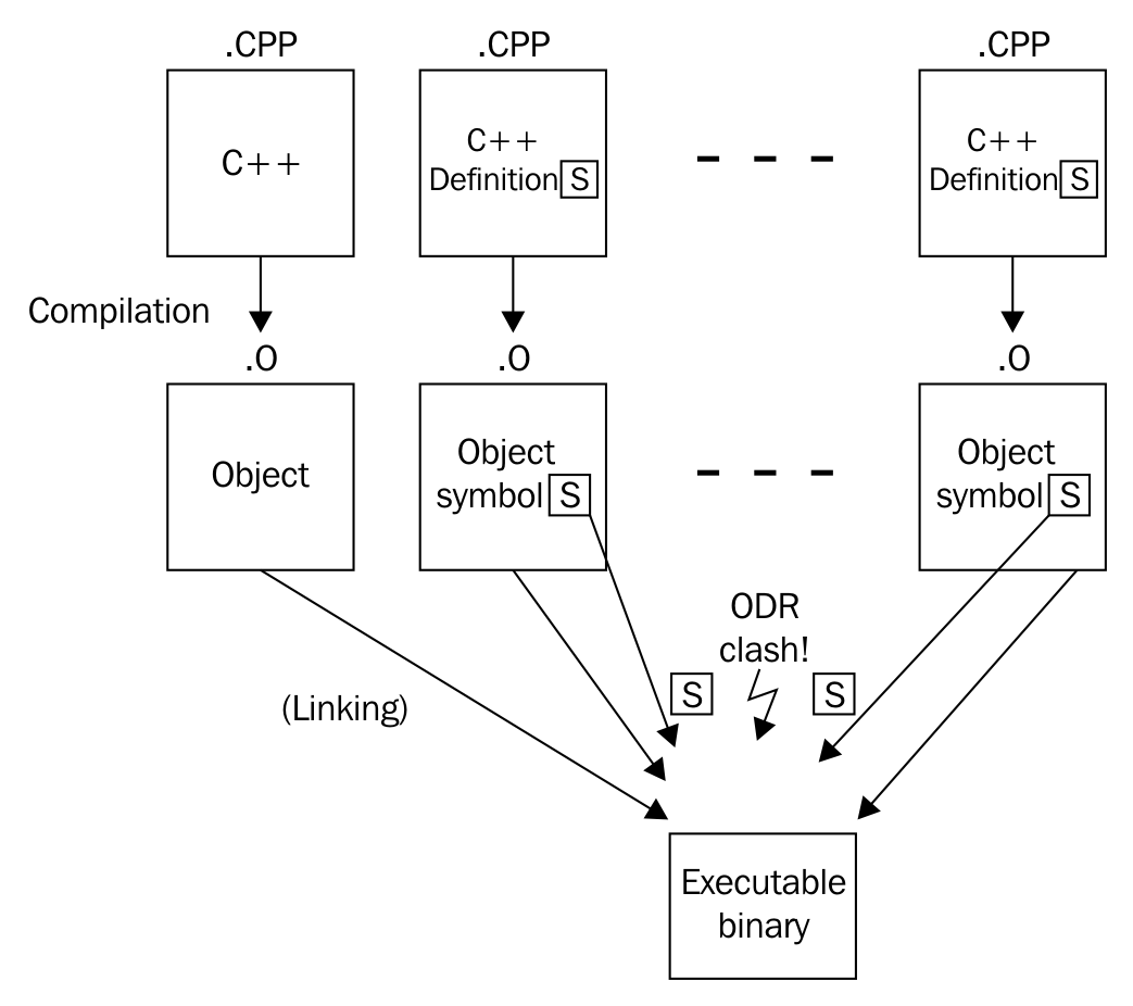
However, if this were the only way, then it would not have been possible to provide header-only libraries. Header-only libraries are very handy because they only need to be included using #include into any C++ program file and then are immediately available. In order to use libraries that are not header-only, the programmer must also adapt the build scripts in order to have the linker link the library modules together with his own module files. Especially for libraries with only very short functions, this is unnecessarily uncomfortable.
For such cases, the inline keyword can be used to make an exception in order to allow multiple definitions of the same symbol in different modules. If the linker finds multiple symbols with the same signature, but they are declared inline, it will just choose the first one and trust that the other symbols have the same definition. That all equal inline symbols are defined completely equal is basically a promise from the programmer.
Regarding our recipe example, the linker will find the process_monitor::standard_string symbol in every module that includes foo_lib.hpp. Without the inline keyword, it would not know which one to choose, so it would abort and report an error. The same applies to the global_process_monitor symbol. Which one is the right one?
After declaring both the symbols inline, it will just accept the first occurrence of each symbol and drop all the others.
Before C++17, the only clean way would be to provide this symbol via an additional C++ module file, which would force our library users to include this file in the linking step.
The inline keyword traditionally also has another function. It tells the compiler that it can eliminate the function call by taking its implementation and directly putting it where it was called. This way, the calling code contains one function call less, which can often be considered faster. If the function is very short, the resulting assembly will also be shorter (assuming that the number of instructions that do the function call, saving and restoring the stack, and so on, is higher than the actual payload code). If the inlined function is very long, the binary size will grow and this might sometimes not even lead to faster code in the end.
Therefore, the compiler will only use the inline keyword as a hint and might eliminate function calls by inlining them. But it can also inline some functions without the programmer having it declared inline.
One possible workaround before C++17 was providing a static function, which returns a reference to a static object:
class foo {
public:
static std::string& standard_string() {
static std::string s {"some standard string"};
return s;
}
};
This way, it is completely legal to include the header file in multiple modules but still getting access to exactly the same instance everywhere. However, the object is not constructed immediately at the start of program but only on the first call of this getter function. For some use cases, this is indeed a problem. Imagine that we want the constructor of the static, globally available object to do something important at program start (just as our reciple example library class), but due to the getter being called near the end of the program, it is too late.
Another workaround is to make the non-template class foo a template class, so it can profit from the same rules as templates.
Both strategies can be avoided in C++17.
Since C++11, there are variadic template parameter packs, which enable implementing functions that accept arbitrarily many parameters. Sometimes, these parameters are all combined into one expression in order to derive the function result from that. This task became really easy with C++17, as it comes with fold expressions.
Let's implement a function that takes arbitrarily many parameters and returns their sum:
template <typename ... Ts>
auto sum(Ts ... ts);
template <typename ... Ts>
auto sum(Ts ... ts)
{
return (ts + ...);
}
int the_sum {sum(1, 2, 3, 4, 5)}; // Value: 15
std::string a {"Hello "};
std::string b {"World"};
std::cout << sum(a, b) << 'n'; // Output: Hello World
What we just did was a simple recursive application of a binary operator (+) to its parameters. This is generally called folding. C++17 comes with fold expressions, which help expressing the same idea with less code.
This kind of expression is called unary fold. C++17 supports folding parameter packs with the following binary operators: +, -, *, /, %, ^, &, |, =, <, >, <<, >>, +=, -=, *=, /=, %=, ^=, &=, |=, <<=, >>=, ==, !=, <=, >=, &&, ||, ,, .*, ->*.
By the way, in our example code, it does not matter if we write (ts + …) or (… + ts); both work. However, there is a difference that may be relevant in other cases--if the … dots are on the right-hand side of the operator, the fold is called a right fold. If they are on the left-hand side, it is a left fold.
In our sum example, a unary left fold expands to 1 + (2 + (3 + (4 + 5))), while a unary right fold will expand to (((1 + 2) + 3) + 4) + 5. Depending on the operator in use, this can make a difference. When adding numbers, it does not.
In case someone calls sum() with no arguments, the variadic parameter pack contains no values that could be folded. For most operators, this is an error (for some, it is not; we will see this in a minute). We then need to decide if this should stay an error or if an empty sum should result in a specific value. The obvious idea is that the sum of nothing is 0.
This is how it’s done:
template <typename ... Ts>
auto sum(Ts ... ts)
{
return (ts + ... + 0);
}
This way, sum() evaluates to 0, and sum(1, 2, 3) evaluates to (1 + (2 + (3 + 0))). Such folds with an initial value are called binary folds.
Again, it works if we write (ts + ... + 0), or (0 + ... + ts), but this makes the binary fold a binary right fold or a binary left fold again. Check out the following diagram:
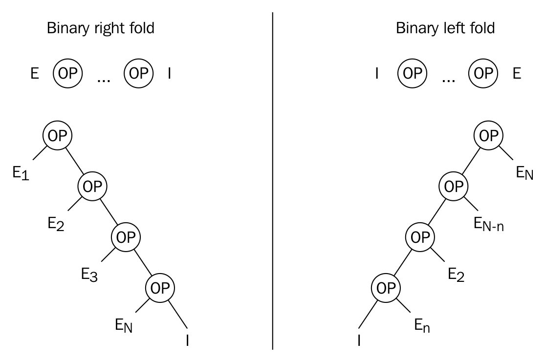
When using binary folds in order to implement the no-argument case, the notion of an identity element is often important--in this case, adding a 0 to any number changes nothing, which makes 0 an identity element. Because of this property, we can add a 0 to any fold expression with the operators + or -, which leads to the result 0 in case there are no parameters in the parameter pack. From a mathematical point of view, this is correct. From an implementation view, we need to define what is correct, depending on what we need.
The same principle applies to multiplication. Here, the identity element is 1:
template <typename ... Ts>
auto product(Ts ... ts)
{
return (ts * ... * 1);
}
The result of product(2, 3) is 6, and the result of product() without parameters is 1.
The logical and (&&) and or (||) operators come with built-in identity elements. Folding an empty parameter pack with && results in true, and folding an empty parameter pack with || results in false.
Another operator that defaults to a certain expression when applied on empty parameter packs is the comma operator (,), which then defaults to void().
In order to ignite some inspiration, let's have a look at some more little helpers that we can implement using this feature.
How about a function that tells whether some range contains at least one of the values we provide as variadic parameters:
template <typename R, typename ... Ts>
auto matches(const R& range, Ts ... ts)
{
return (std::count(std::begin(range), std::end(range), ts) + ...);
}
The helper function uses the std::count function from the STL. This function takes three parameters: the first two parameters are the begin and end iterators of some iterable range, and as the third parameter, it takes a value which will be compared to all the items of the range. The std::count method then returns the number of all the elements within the range that are equal to the third parameter.
In our fold expression, we always feed the begin and end iterators of the same parameter range into the std::count function. However, as the third parameter, each time we put one other parameter from the parameter pack into it. In the end, the function sums up all the results and returns it to the caller.
We can use it like this:
std::vector<int> v {1, 2, 3, 4, 5};
matches(v, 2, 5); // returns 2
matches(v, 100, 200); // returns 0
matches("abcdefg", 'x', 'y', 'z'); // returns 0
matches("abcdefg", 'a', 'd', 'f'); // returns 3
As we can see, the matches helper function is quite versatile--it can be called on vectors or even on strings directly. It would also work on initializer lists, on instances of std::list, std::array, std::set, and so on!
Let's write a helper that inserts an arbitrary number of variadic parameters into an std::set and returns if all the insertions are successful:
template <typename T, typename ... Ts>
bool insert_all(T &set, Ts ... ts)
{
return (set.insert(ts).second && ...);
}
So, how does this work? The insert function of std::set has the following signature:
std::pair<iterator, bool> insert(const value_type& value);
The documentation says that when we try to insert an item, the insert function will return an iterator and a bool variable in a pair. The bool value is true if the insertion is successful. If it is successful, the iterator points to the new element in the set. Otherwise, the iterator points to the existing item, which would collide with the item to be inserted.
Our helper function accesses the .second field after insertion, which is just the bool variable that reflects success or fail. If all the insertions lead to true in all the return pairs, then all the insertions were successful. The fold expression combines all the insertion results with the && operator and returns the result.
We can use it like this:
std::set<int> my_set {1, 2, 3};
insert_all(my_set, 4, 5, 6); // Returns true
insert_all(my_set, 7, 8, 2); // Returns false, because the 2 collides
Note that if we try to insert, for example, three elements, but the second element can already not be inserted, the && ... fold will short-circuit and stop inserting all the other elements:
std::set<int> my_set {1, 2, 3};
insert_all(my_set, 4, 2, 5); // Returns false
// set contains {1, 2, 3, 4} now, without the 5!
If we can check if one variable is within some specific range, we can also do the same thing with multiple variables using fold expressions:
template <typename T, typename ... Ts>
bool within(T min, T max, Ts ...ts)
{
return ((min <= ts && ts <= max) && ...);
}
The expression, (min <= ts && ts <= max), does tell for every value of the parameter pack if it is between min and max (including min and max). We choose the && operator to reduce all the Boolean results to a single one, which is only true if all the individual results are true.
This is how it looks in action:
within( 10, 20, 1, 15, 30); // --> false
within( 10, 20, 11, 12, 13); // --> true
within(5.0, 5.5, 5.1, 5.2, 5.3) // --> true
Interestingly, this function is very versatile because the only requirement it imposes on the types we use is that they are comparable with the <= operator. And this requirement is also fulfilled by std::string, for example:
std::string aaa {"aaa"};
std::string bcd {"bcd"};
std::string def {"def"};
std::string zzz {"zzz"};
within(aaa, zzz, bcd, def); // --> true
within(aaa, def, bcd, zzz); // --> false
It's also possible to write a helper that does not reduce any results but processes multiple actions of the same kind. Like inserting items into an std::vector, which does not return any results (std::vector::insert() signalizes error by throwing exceptions):
template <typename T, typename ... Ts>
void insert_all(std::vector<T> &vec, Ts ... ts)
{
(vec.push_back(ts), ...);
}
int main()
{
std::vector<int> v {1, 2, 3};
insert_all(v, 4, 5, 6);
}
Note that we use the comma (,) operator in order to expand the parameter pack into individual vec.push_back(...) calls without folding the actual result. This function also works nicely with an empty parameter pack because the comma operator has an implicit identity element, void(), which translates to do nothing.
We will cover the following recipes in this chapter:
A lot of novice C++ programmers learn about std::vector, that it basically works like an automatically growing array, and stop right there. Later, they only lookup its documentation in order to see how to do very specific things, for example, removing items. Using STL containers like this will only scratch the surface of how much they help writing clean, maintainable, and fast code.
This section is all about removing items from in-between a vector instance. When an item disappears from a vector, and sits somewhere in the middle between other items, then all items right from it must move one slot to the left (which gives this task a runtime cost within O(n)). Many novice programmers will do that using a loop, since it is also not really a hard thing to do. Unfortunately, they will potentially ignore a lot of optimization potential while doing that. And in the end, a hand crafted loop is neither faster, nor prettier to read than the STL way, which we will see next.
In this section, we are filling an std::vector instance with some example integers, and then prune some specific items away from it. The way we are doing it is considered the correct way of removing multiple items from a vector.
#include <iostream>
#include <vector>
#include <algorithm>
using namespace std;
int main()
{
vector<int> v {1, 2, 3, 2, 5, 2, 6, 2, 4, 8};
const auto new_end (remove(begin(v), end(v), 2));
v.erase(new_end, end(v));
for (auto i : v) {
cout << i << ", ";
}
cout << 'n';
const auto odd ([](int i) { return i % 2 != 0; });
v.erase(remove_if(begin(v), end(v), odd), end(v));
v.shrink_to_fit();
for (auto i : v) {
cout << i << ", ";
}
cout << 'n';
}
$ ./main
1, 3, 5, 6, 4, 8,
6, 4, 8,
What became obvious in the recipe is that when removing items from the middle of a vector, they first need to be removed and then erased. At least the functions we used have names like this. This is admittedly confusing, but let's have a closer look at it to make sense of these steps.
The code which removes all values of 2 from the vector, looked like this:
const auto new_end (remove(begin(v), end(v), 2));
v.erase(new_end, end(v));
The std::begin and std::end functions both accept a vector instance as parameter, and return us iterators, which point to the first item, and past the last item, just as sketched in the upcoming diagram.
After feeding these and the value 2 to the std::remove function, it will move the non-2 values forward, just like we could do that with a manually programmed loop. The algorithm will strictly preserve the order of all non-2 values while doing that. A quick look at the illustration might be a bit confusing. In step 2, there still is a value of 2, and the vector should have become shorter, as there were four values of 2, which all ought to be removed. Instead, the 4 and the 8 which were in the initial array, are duplicated. What's that?
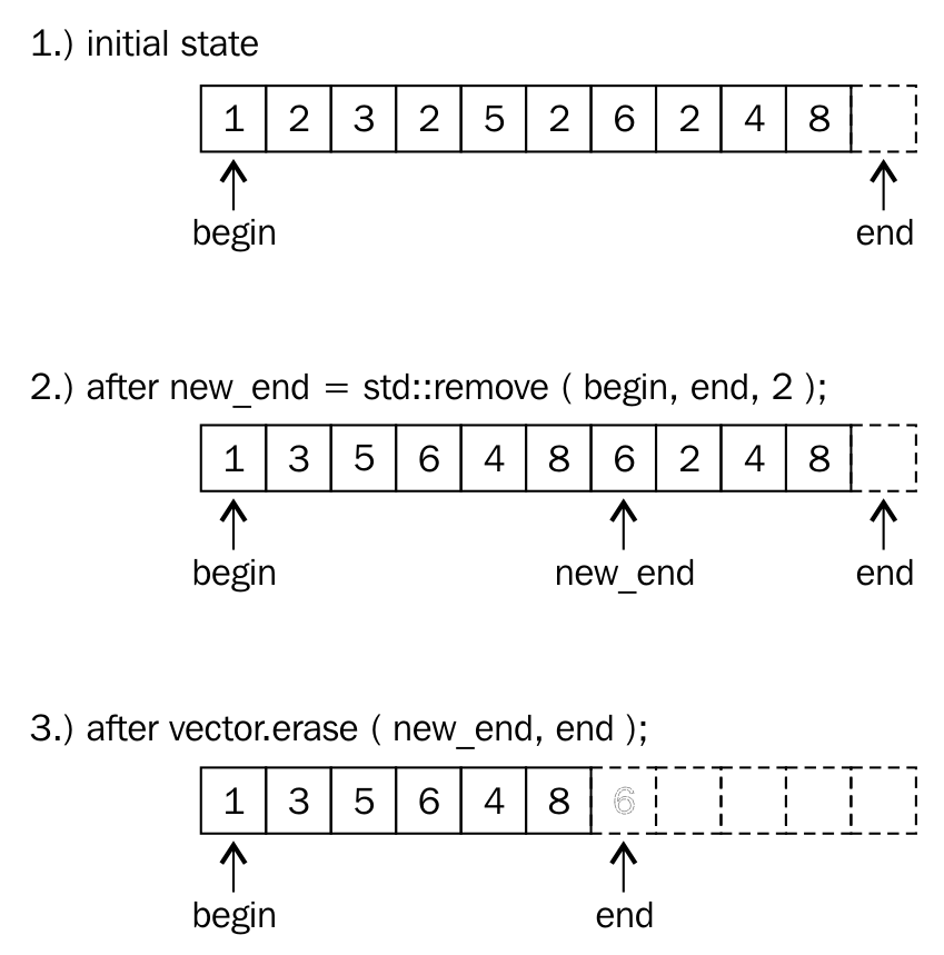
Let's only take a look at all the items, which are within the range and which spans from the begin iterator on the illustration, to the new_end iterator. The item, to which the new_end iterator points, is the first item past the range, so it's not included. Just concentrating on that region (these are only the items from 1 to including 8), we realize that this is the correct range from which all values of 2 are removed.
This is where the erase call comes into play: We must tell the vector that it shall not consider all items from new_end to end to be items of the vector any longer. This order is easy to follow for the vector, as it can just point its end iterator to the position of new_end and it's done. Note that new_end was the return value of the std::remove call, so we can just use that.
Afterward, the vector looks like in step 3 of the diagram: it's considered smaller now. The old items which are now out of the range, are still in memory.
In order to make the vector occupy only as much memory as it needs, we make the shrink_to_fit call in the end. During that call, it allocates exactly as much memory as needed, moves over all the items and deletes the larger chunk we don't need any longer.
In step 8, we define a predicate function and use it with std::remove_if in only one step. This works, because whatever iterator the remove function returns, it is safe to be used in the vector's erase function. Even if no odd item was found, the std::remove_if function will do just nothing, and return the end iterator. Then, a call like v.erase(end, end); also does nothing, hence it is harmless.
The std::remove function also works on other containers. When used with std::array, note that it does not support the second step of calling erase, because they do not have automatic size handling. Just because std::remove effectively only moves items around and does not perform their actual deletion, it can also be used on data structures such as arrays that do not support resizing. In the array case, one could overwrite the values past the new end iterator with sentinel values such as '' for strings, for example.
Deleting items from somewhere in the middle of an std::vector takes O(n) time. This is because the resulting gap from removing an item must be filled by moving all the items which come after the gap one slot to the left.
While moving items around like this, which might be expensive if they are complex and/or very large and include many items, we preserve their order. If preserving the order is not important, we can optimize this, as this section shows.
In this section, we will fill an std::vector instance with some example numbers, and implement a quick remove function, which removes any item from a vector in O(1) time.
#include <iostream>
#include <vector>
#include <algorithm>
int main()
{
std::vector<int> v {123, 456, 789, 100, 200};
quick_remove_at(v, 2);
for (int i : v) {
std::cout << i << ", ";
}
std::cout << 'n';
quick_remove_at(v, std::find(std::begin(v), std::end(v), 123));
for (int i : v) {
std::cout << i << ", ";
}
std::cout << 'n';
}
template <typename T>
void quick_remove_at(std::vector<T> &v, std::size_t idx)
{
if (idx < v.size()) {
v[idx] = std::move(v.back());
v.pop_back();
}
}
template <typename T>
void quick_remove_at(std::vector<T> &v,
typename std::vector<T>::iterator it)
{
if (it != std::end(v)) {
*it = std::move(v.back());
v.pop_back();
}
}
$ ./main
123, 456, 200, 100,
100, 456, 200,
The quick_remove_at function removes items pretty quickly without touching too many other items. It does this in a relatively creative way: It kind of swaps the actual item, which shall be removed with the last item in the vector. Although the last item has no connection to the actually selected item, it is in a special position: Removing the last item is cheap! The vector's size just needs to be shrunk down by one slot, and that's it. No items are moved during that step. Have a look at the following diagram which helps imaging how this happens:
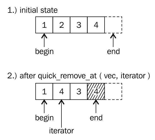
Both the steps in the recipe code look like this:
v.at(idx) = std::move(v.back());
v.pop_back();
This is the iterator version, which looks nearly identical:
*it = std::move(v.back());
v.pop_back();
Logically, we swap the selected item and the last one. But the code does not swap items, it moves the last one over the first one. Why? If we swapped the items, then we would have to store the selected item in a temporary variable, move the last item to the selected item, and then store the temporary value in the last slot again. This seems useless, as we are just about to delete the last item anyway.
Ok, fine, so the swap is useless, and a one-way overwrite is a better thing to do. Having seen that, we can argue that this step could also be performed with a simple *it = v.back();, right? Yes, this would be completely correct, but imagine we stored some very large strings in every slot, or even another vector or map--in that situation, that little assignment would lead to a very expensive copy. The std::move call in between is just an optimization: In the example case of strings, the string item internally points to a large string in the heap. We do not need to copy that. Instead, when moving a string, the destination of the move gets to point at the string data of the other. The move source item is left intact, but in a useless state, which is fine because we are removing it anyway.
The std::vector is probably the most widely used container in the STL, because it holds data just like an array, and adds a lot of comfort around that representation. However, wrong access to a vector can still be dangerous. If a vector contains 100 elements, and by accident our code tries to access an element at index 123, this is obviously bad. Such a program could just crash, which might be the best case, because that behavior would make it very obvious that there is a bug! If it does not crash, we might observe that the program just behaves strangely from time to time, which could lead to even more headaches than a crashing program. The experienced programmer might add some checks before any directly indexed vector access. Such checks do not increase the readability of the code, and many people do not know that std::vector already has built-in bound checks!
In this section, we will use the two different ways to access an std::vector, and then see how we can utilize them to write safer programs without decreasing readability.
#include <iostream>
#include <vector>
using namespace std;
int main()
{
const size_t container_size {1000};
vector<int> v (container_size, 123);
cout << "Out of range element value: "
<< v[container_size + 10] << 'n';
cout << "Out of range element value: "
<< v.at(container_size + 10) << 'n';
}
Out of range element value: -726629391
terminate called after throwing an instance of 'std::out_of_range'
what(): array::at: __n (which is 1010) >= _Nm (which is 1000)
Aborted (core dumped)
The std::vector provides the [] operator and the at function, and they basically do exactly the same job. The at function, however, performs additional bounds checks and throws an exception if the vector bounds are exceeded. This is super useful in situations like ours, but also makes the program a little bit slower.
Especially when doing numeric computations with indexed members which need to be really fast, it is advantageous to stick to [] indexed access. In any other situation, the at function helps uncovering bugs with usually negligible performance loss.
Of course, we can handle out of bounds accesses, instead of letting the whole app crash. In order to handle it, we catch the exception, in case it was thrown by the at function. Catching such an exception is simple. We just surround the at call with a try block and define the error handling in a catch block.
try {
std::cout << "Out of range element value: "
<< v.at(container_size + 10) << 'n';
} catch (const std::out_of_range &e) {
std::cout << "Ooops, out of range access detected: "
<< e.what() << 'n';
}
Arrays and vectors do not sort their payload objects themselves. But if we need that, this does not mean that we always have to switch to data structures, which were designed to do that automatically. If an std::vector is perfect for our use case, it is still very simple and practical to add items to it in a sorting manner.
In this section, we will fill an std::vector with random words, sort it, and then insert more words while keeping the vector's sorted word order intact.
#include <iostream>
#include <vector>
#include <string>
#include <algorithm>
#include <iterator>
#include <cassert>
using namespace std;
int main()
{
vector<string> v {"some", "random", "words",
"without", "order", "aaa",
"yyy"};
assert(false == is_sorted(begin(v), end(v)));
sort(begin(v), end(v));
assert(true == is_sorted(begin(v), end(v)));
insert_sorted(v, "foobar");
insert_sorted(v, "zzz");
void insert_sorted(vector<string> &v, const string &word)
{
const auto insert_pos (lower_bound(begin(v), end(v), word));
v.insert(insert_pos, word);
}
for (const auto &w : v) {
cout << w << " ";
}
cout << 'n';
}
aaa foobar order random some without words yyy zzz
The whole program is constructed around the insert_sorted function, which does what this section is about: For any new string, it locates the position in the sorted vector, at which it must be inserted, in order to preserve the order of the strings in the vector. However, we assume that the vector was sorted before. Otherwise, this would not work.
The locating step is done by the STL function lower_bound, which accepts three arguments. The first two denote beginning and end of the underlying range. The range is our vector of words in this case. The third argument is the word, which shall be inserted. The function then finds the first item in the range, which is greater than or equal to that third parameter and returns an iterator pointing to it.
Having the right position at hand, we gave it to the std::vector member method insert, which accepts just two arguments. The first argument is an iterator, which points to the position in the vector, at which the second parameter shall be inserted. It appears very handy that we can use the same iterator, which just dropped out of the lower_bound function. The second argument is, of course, the item to be inserted.
The insert_sorted function is pretty generic. If we generalize the types of its parameters, it will also work on other container payload types, and even on other containers such as std::set, std::deque, std::list, and so on! (Note that set has its own lower_bound member function that does the same as std::lower_bound, but is more efficient because it is specialized for sets.)
template <typename C, typename T>
void insert_sorted(C &v, const T &item)
{
const auto insert_pos (lower_bound(begin(v), end(v), item));
v.insert(insert_pos, item);
}
When trying to switch the type of the vector in the recipe from std::vector to something else, note that not all containers support std::sort. That algorithm requires random access containers, which std::list, for example, does not fulfill.
Sometimes we want to fill a map with key-value pairs and while filling the map up, we might run into two different cases:
We could just naively use the insert or emplace methods of map and see if they succeed. If it doesn't, we have case 2 and modify the existing item. In both cases, insert and emplace create the item which we try to insert, and in case 2 the freshly created item is dropped. We get a useless constructor call in both cases.
Since C++17, there is the try_emplace function, which enables us to create items only conditionally upon insertion. Let's implement a program that takes a list of billionaires and constructs a map that tells us the number of billionaires per country. In addition to that, it stores the wealthiest person in every country. Our example will not contain expensive to create items, but whenever we find ourselves in such a situation in real-life projects, we know how to master it with try_emplace.
In this section, we will implement an application that creates a map from a list of billionaires. The map maps from each country to a reference to the wealthiest person in that country and a counter that tells how many billionaires that country has.
#include <iostream>
#include <functional>
#include <list>
#include <map>
using namespace std;
struct billionaire {
string name;
double dollars;
string country;
};
int main()
{
list<billionaire> billionaires {
{"Bill Gates", 86.0, "USA"},
{"Warren Buffet", 75.6, "USA"},
{"Jeff Bezos", 72.8, "USA"},
{"Amancio Ortega", 71.3, "Spain"},
{"Mark Zuckerberg", 56.0, "USA"},
{"Carlos Slim", 54.5, "Mexico"},
// ...
{"Bernard Arnault", 41.5, "France"},
// ...
{"Liliane Bettencourt", 39.5, "France"},
// ...
{"Wang Jianlin", 31.3, "China"},
{"Li Ka-shing", 31.2, "Hong Kong"}
// ...
};
map<string, pair<const billionaire, size_t>> m;
for (const auto &b : billionaires) {
auto [iterator, success] = m.try_emplace(b.country, b, 1);
if (!success) {
iterator->second.second += 1;
}
}
for (const auto & [key, value] : m) {
const auto &[b, count] = value;
cout << b.country << " : " << count
<< " billionaires. Richest is "
<< b.name << " with " << b.dollars
<< " B$n";
}
}
$ ./efficient_insert_or_modify
China : 1 billionaires. Richest is Wang Jianlin with 31.3 B$
France : 2 billionaires. Richest is Bernard Arnault with 41.5 B$
Hong Kong : 1 billionaires. Richest is Li Ka-shing with 31.2 B$
Mexico : 1 billionaires. Richest is Carlos Slim with 54.5 B$
Spain : 1 billionaires. Richest is Amancio Ortega with 71.3 B$
USA : 4 billionaires. Richest is Bill Gates with 86 B$
The whole recipe revolves around the try_emplace function of std::map, which is a new C++17 addition. It has the following signature:
std::pair<iterator, bool> try_emplace(const key_type& k, Args&&... args);
Thus, the key being inserted is parameter k and the associated value is constructed from the parameter pack args. If we succeed in inserting the item, then the function returns an iterator, which points to the new node in the map, paired with a Boolean value being set to true. If the insertion was not successful, the Boolean value in the return pair is set to false, and the iterator points to the item with which the new item would clash.
This characteristic is very useful in our case--when we see a billionaire from a specific country for the first time, then this country is not a key in the map yet. In that case, we must insert it, accompanied with a new counter being set to 1. If we did see a billionaire from a specific country already, we have to get a reference to its existing counter, in order to increment it. This is exactly what happened in step 6:
if (!success) {
iterator->second.second += 1;
}
The whole program still works if we switch the type of the map from std::map to std::unordered_map. This way, we can simply switch from one implementation to another, which has different performance characteristics. In this recipe, the only observable difference is that the billionaire map is not printed in alphabetical order any longer, because hash maps do not order their objects the same way as search trees do.
Looking up items in an std::map takes O(log(n)) time. This is the same for inserting new items, because the position where to insert them must be looked up. Naive insertion of M new items would thus take O(M * log(n)) time.
In order to make this more efficient, std::map insertion functions accept an optional insertion hint parameter. The insertion hint is basically an iterator, which points near the future position of the item that is to be inserted. If the hint is correct, then we get amortized O(1) insertion time.
In this section, we will insert multiple items into an std::map, and use insertion hints for that, in order to reduce the number of lookups.
#include <iostream>
#include <map>
#include <string>
int main()
{
std::map<std::string, size_t> m {{"b", 1}, {"c", 2}, {"d", 3}};
auto insert_it (std::end(m));
for (const auto &s : {"z", "y", "x", "w"}) {
insert_it = m.insert(insert_it, {s, 1});
}
m.insert(std::end(m), {"a", 1});
for (const auto & [key, value] : m) {
std::cout << """ << key << "": " << value << ", ";
}
std::cout << 'n';
}
"a": 1, "b": 1, "c": 2, "d": 3, "w": 1, "x": 1, "y": 1, "z": 1,
The only difference to normal map insertions in this recipe was the additional hint iterator. And we spoke about correct and wrong hints.
A correct hint will point to an existing element, which is greater than the element to be inserted so that the newly inserted key will be just before the hint. If this does not apply for the hint the user provided during an insertion, the insert function will fall back to a nonoptimized insertion, yielding O(log(n)) performance again.
For the first insertion, we got the end iterator of the map, because we had no better hint to start with. After installing a "z" in the tree, we knew that installing "y" will insert a new item just in front of the "z", which qualified it to be a correct hint. This applies to "x" as well, if put into the tree after inserting the "y", and so on. This is why it is possible to use the iterator, which was returned by the last insertion for the next insertion.
Interestingly, a wrong hint does not even destroy or disturb the order of the items in the map, so how does that even work, and what did that mean, that the insertion time is amortized O(1)?
The std::map is usually implemented using a binary search tree. When inserting a new key into a search tree, it is compared against the keys of the other nodes, beginning from the top. If the key is smaller or larger than the key of one node, then the search algorithm branches left or right to go down to the next deeper node. While doing that, the search algorithm will stop at the point where it reached the maximum depth of the current tree, where it will put the new node with its key. It is possible that this step destroyed the tree's balance, so it will also correct that using a re-balancing algorithm afterward as a housekeeping task.
When we insert items into a tree with key values which are direct neighbors of each other (just as the integer 1 is a neighbor of the integer 2, because no other integer fits between them), they can often also be inserted just next to each other in the tree, too. It can easily be checked if this is true for a certain key and an accompanying hint. And if this situation applies, the search algorithm step can be omitted, which spares some crucial runtime. Afterward, the re-balancing algorithm might nevertheless have to be run.
When such an optimization can often be done, but not always, this can still lead to an average performance gain. It is possible to show a resulting runtime complexity which settles down after multiple insertions, and then it's called amortized complexity.
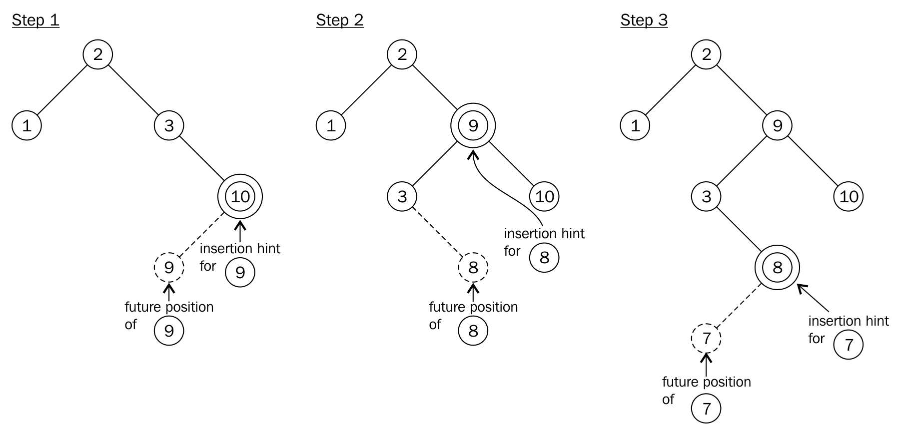
If the insertion hint is wrong, the insertion function will simply waive the hint and start over using the search algorithm. This works correctly but is obviously slower.
Since the std::map data structure maps from keys to values in a way that the keys are always unique and sorted, it is of crucial value that users cannot modify the keys of map nodes that are already inserted. In order to prevent the user from modifying the key items of perfectly sorted map nodes, the const qualifier is added to the key type.
This kind of restriction is perfectly sane because it makes it harder for the user to use std::map the wrong way. But what shall we do if we really need to change the keys of some map items?
Prior to C++17, we had to remove the items of which we need to change the key value from the tree, in order to reinsert them. The downside of this approach is that this always needlessly reallocates some memory, which sounds bad in terms of performance.
Since C++17, we can remove and reinsert map nodes without any reallocation of memory. We will see how that works in this recipe.
We implement a little application that orders the placement of drivers in a fictional race in an std::map structure. While drivers pass each other during the race, we need to change their placement keys, which we do the new C++17 way.
#include <iostream>
#include <map>
using namespace std;
template <typename M>
void print(const M &m)
{
cout << "Race placement:n";
for (const auto &[placement, driver] : m) {
cout << placement << ": " << driver << 'n';
}
}
int main()
{
map<int, string> race_placement {
{1, "Mario"}, {2, "Luigi"}, {3, "Bowser"},
{4, "Peach"}, {5, "Yoshi"}, {6, "Koopa"},
{7, "Toad"}, {8, "Donkey Kong Jr."}
};
print(race_placement);
{
auto a (race_placement.extract(3));
auto b (race_placement.extract(8));
swap(a.key(), b.key());
race_placement.insert(move(a));
race_placement.insert(move(b));
}
print(race_placement);
}
$ ./mapnode_key_modification
Race placement:
1: Mario
2: Luigi
3: Bowser
4: Peach
5: Yoshi
6: Koopa
7: Toad
8: Donkey Kong Jr.
Race placement:
1: Mario
2: Luigi
3: Donkey Kong Jr.
4: Peach
5: Yoshi
6: Koopa
7: Toad
8: Bowser
In C++17, std::map got a new member function extract. It comes in two flavors:
node_type extract(const_iterator position);
node_type extract(const key_type& x);
In this recipe, we used the second one, which accepts a key and then finds and extracts the map node that matches the key parameter. The first one accepts an iterator, which implies that it is faster because it doesn't need to search for the item.
If we try to extract an item that doesn't exist with the second method (the one that searches using a key), it returns an empty node_type instance. The empty() member method returns us a Boolean value that tells whether a node_type instance is empty or not. Accessing any other method on an empty instance leads to undefined behavior.
After extracting nodes, we were able to modify their keys using the key() method, which gives us nonconst access to the key, although keys are usually const.
Note that in order to reinsert the nodes into the map again, we had to move them into the insert function. This makes sense because extract is all about avoiding unnecessary copies and allocations. Note that while we move a node_type instance, this does not result in actual moves of any of the container values.
Map nodes that have been extracted using the extract method are actually very versatile. We can extract nodes from a map instance and insert it into any other map or even multimap instance. It does also work between unordered_map and unordered_multimap instances, as well as with set/multiset and respective unordered_set/unordered_multiset.
In order to move items between different map/set structures, the types of key, value, and allocator need to be identical. Note that even if that is the case, we cannot move nodes from a map to an unordered_map, or from a set to an unordered_set.
If we use std::unordered_map instead of std::map, we have a different degree of freedom for the choice of the key type which shall be used. std::map demands that there is a natural order between all key items. This way, items can be sorted. But what if we want, for example, mathematical vectors as a key type? There is no meaning in a smaller < relation for such types, as a vector (0, 1) is not smaller or larger than (1, 0). They just point in different directions. This is completely fine for std::unordered_map because it will not distinguish items via their smaller/greater ordering relationship but via hash values. The only thing we need to do is to implement a hash function for our own type, and an equal to == operator implementation, which tells whether two objects are identical. This section will demonstrate this in an example.
In this section, we will define a simple coord struct, which has no default hash function, so we need to define it ourselves. Then we put it to use by mapping coord values to numbers.
#include <iostream>
#include <unordered_map>
struct coord {
int x;
int y;
};
bool operator==(const coord &l, const coord &r)
{
return l.x == r.x && l.y == r.y;
}
namespace std
{
template <>
struct hash<coord>
{
using argument_type = coord;
using result_type = size_t;
result_type operator()(const argument_type &c) const
{
return static_cast<result_type>(c.x)
+ static_cast<result_type>(c.y);
}
};
}
int main()
{
std::unordered_map<coord, int> m {{{0, 0}, 1}, {{0, 1}, 2},
{{2, 1}, 3}};
for (const auto & [key, value] : m) {
std::cout << "{(" << key.x << ", " << key.y
<< "): " << value << "} ";
}
std::cout << 'n';
}
$ ./custom_type_unordered_map
{(2, 1): 3} {(0, 1): 2} {(0, 0): 1}
Usually, when we instantiate a hash-based map implementation like std::unordered_map, we write:
std::unordered_map<key_type, value_type> my_unordered_map;
It is not too obvious that there happens a lot of magic in the background when the compiler creates our std::unordered_map specialization. So, let's have a look at the complete template-type definition of it:
template<
class Key,
class T,
class Hash = std::hash<Key>,
class KeyEqual = std::equal_to<Key>,
class Allocator = std::allocator< std::pair<const Key, T> >
> class unordered_map;
The first two template types are those we filled with coord and int, which is the simple and obvious part. The other three template types are optional, as they are automatically filled with existing standard template classes, which themselves take template types. Those are fed with our choice for the first two parameters as default values.
Regarding this recipe, the class Hash template parameter is the interesting one: when we do not explicitly define anything else, it is going to be specialized on std::hash<key_type>. The STL already contains std::hash specializations for a lot of types such as std::hash<std::string>, std::hash<int>, std::hash<unique_ptr>, and many more. These classes know how to deal with such specific types in order to calculate optimal hash values from them.
However, the STL does not know how to calculate a hash value from our struct coord, yet. So what we did was to just define another specialization, which knows how to deal with it. The compiler can now go through the list of all std::hash specializations it knows, and will find our implementation to match it with the type we provided as key type.
If we did not add a new std::hash<coord> specialization, and named it my_hash_type instead, we could still use it with the following instantiation line:
std::unordered_map<coord, value_type, my_hash_type> my_unordered_map;
That is obviously more to type, and not as nice to read as when the compiler finds the right hashing implementation itself.
std::set is a strange container: It kind of works like std::map, but it contains only keys as values, no key-value pairs. So it can hardly be used as a way to map values of one type to the other. Seemingly, just because there are less obvious use cases for it, a lot of developers do not even know about its existence. Then they start to implement things themselves, although std::set would be of great help in some of these situations.
This section shows how to put std::set to use in an example where we collect potentially many different items, in order to filter them and output a selection of the unique ones.
In this section, we will read a stream of words from the standard input. All unique words are put into an std::set instance. This way we can then enumerate all unique words from the stream.
#include <iostream>
#include <set>
#include <string>
#include <iterator>
using namespace std;
int main()
{
set<string> s;
istream_iterator<string> it {cin};
istream_iterator<string> end;
copy(it, end, inserter(s, s.end()));
for (const auto word : s) {
cout << word << ", ";
}
cout << 'n';
}
$ echo "a a a b c foo bar foobar foo bar bar" | ./program
a, b, bar, c, foo, foobar,
This program consists of two interesting parts. The first part is using std::istream_iterator to access the user input, and the second part is to combine this with our std::set instance using the std::copy algorithm, after we wrapped it into an std::inserter instance! It might look surprising that there is only one line of code which does all the work of tokenizing the input, putting it into the alphabetically sorted set, and dropping all duplicates.
This class is really interesting in cases where we want to process masses of data of the same type from a stream, which is exactly the case in this recipe: we parse the whole input word by word and put it into the set in the form of std::string instances.
The std::istream_iterator takes one template parameter. That is the type of the input we want to have. We chose std::string because we assume text words, but it could also have been float numbers, for example. It can basically be every type for which it is possible to write cin >> var;. The constructor accepts an istream instance. The standard input is represented by the global input stream object std::cin, which is an acceptable istream parameter in this case.
istream_iterator<string> it {cin};
The input stream iterator it which we have instantiated, is able to do two things: when it is dereferenced (*it), it yields the current input symbol. As we have typed the iterator to std::string via its template parameter, that symbol will be a string containing one word. When it is incremented (++it), it will jump to the next word, which we can access by dereferencing again.
But wait, we need to be careful after every increment before we dereference it again. If the standard input ran empty, the iterator must not be dereferenced again. Instead, we should terminate the loop in which we dereference the iterator to get at every word. The abort condition, which lets us know that the iterator became invalid, is a comparison with the end iterator. If it == end holds, we are past the end of the input.
We create the end iterator by creating an std::istream_iterator instance with its parameterless standard constructor. It has the purpose of being the counterpart of the comparison which shall act as the abort condition in every iteration:
istream_iterator<string> end;
As soon as std::cin runs empty, our it iterator instance will notice that and make a comparison with end returning true.
We used the it and end pair as input iterators in the std::copy call. The third parameter must be an output iterator. For that, we cannot just take s.begin() or s.end(). In an empty set, both are the same, so we are not even allowed to dereference it, regardless if that is for reading from it or assigning to it.
This is where std::inserter comes into play. It is a function which returns an std::insert_iterator that behaves like an iterator but does something else than what usual iterators do. When we increment it, it does nothing. When we dereference it and assign something to it, it will take the container it is attached to, and insert that value as a new item into it!
When instantiating an std::insert_iterator via std::inserter, two parameters are needed:
auto insert_it = inserter(s, s.end());
The s is our set, and s.end() is an iterator that points to where the new item shall be inserted. For an empty set which we start with, this makes as much sense as s.begin(). When used for other data structures as vectors or lists, that second parameter is crucial for defining where the insert iterator shall insert new items.
In the end, all the action happens during the std::copy call:
copy(input_iterator_begin, input_iterator_end, insert_iterator);
This call pulls the next word token out of std::cin via the input iterator and pushes it into our std::set. Afterward, it increments both iterators, and checks whether the input iterator is equal to the input end iterator counterpart. If it is not, then there are still words left in the standard input, so it will repeat.
Duplicate words are automatically dropped. If the set already contains a specific word, adding it again has no effect. This would be different in an std::multiset as, in contrast, it would accept duplicates.
The std::stack is an adapter class which lets the user push objects onto it like on a real stack of objects, and pop objects down from it again. In this section, we construct a reverse polish notation (RPN) calculator around that data structure, in order to show how to use it.
The RPN is a notation that can be used to express mathematical expressions in a way that is really simple to parse. In RPN, 1 + 2 is 1 2 +. Operands first, then the operation. Another example: (1 + 2) * 3 would be 1 2 + 3 * in RPN and that already shows why it is easier to parse, as we do not need parentheses to define subexpressions.
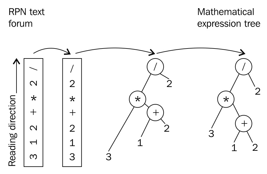
In this section, we will read a mathematical expression in RPN from the standard input, and then feed it into a function that evaluates it. In the end, we print the numeric result back to the user.
#include <iostream>
#include <stack>
#include <iterator>
#include <map>
#include <sstream>
#include <cassert>
#include <vector>
#include <stdexcept>
#include <cmath>
using namespace std;
template <typename IT>
double evaluate_rpn(IT it, IT end)
{
stack<double> val_stack;
auto pop_stack ([&](){
auto r (val_stack.top());
val_stack.pop();
return r;
});
map<string, double (*)(double, double)> ops {
{"+", [](double a, double b) { return a + b; }},
{"-", [](double a, double b) { return a - b; }},
{"*", [](double a, double b) { return a * b; }},
{"/", [](double a, double b) { return a / b; }},
{"^", [](double a, double b) { return pow(a, b); }},
{"%", [](double a, double b) { return fmod(a, b); }},
};
for (; it != end; ++it) {
stringstream ss {*it};
if (double val; ss >> val) {
val_stack.push(val);
}
else {
const auto r {pop_stack()};
const auto l {pop_stack()};
try {
const auto & op (ops.at(*it));
const double result {op(l, r)};
val_stack.push(result);
}
catch (const out_of_range &) {
throw invalid_argument(*it);
}
}
}
return val_stack.top();
}
int main()
{
try {
cout << evaluate_rpn(istream_iterator<string>{cin}, {})
<< 'n';
}
catch (const invalid_argument &e) {
cout << "Invalid operator: " << e.what() << 'n';
}
}
$ echo "3 1 2 + * 2 /" | ./rpn_calculator
4.5
The whole recipe revolves around pushing operands onto the stack until we see an operation in the input. In that situation, we pop the last two operands from the stack again, apply the operation to them, and push the result onto the stack again. In order to understand all of the code in this recipe, it is important to understand how we distinguish operands and operations from the input, how we handle our stack, and how we select and apply the right mathematical operation.
We push items onto the stack, simply using the push function of std::stack:
val_stack.push(val);
Popping values from it looks a bit more complicated because we implemented a lambda for that, which captures a reference to the val_stack object. Let's look at the same code, enhanced with some more comments:
auto pop_stack ([&](){
auto r (val_stack.top()); // Get top value copy
val_stack.pop(); // Throw away top value
return r; // Return copy
});
This lambda is necessary to get the top value of the stack and remove it from there in one step. The interface of std::stack is not designed in a way which would allow doing that in a single call. However, defining a lambda is quick and easy, so we can now get values like this:
double top_value {pop_stack()};
In the main loop of evaluate_rpn, we take the current string token from the iterator and then see whether it is an operand or not. If the string can be parsed into a double variable, then it is a number, and hence also an operand. We consider everything which is not easily parseable as a number (such as "+", for example) to be an operation.
The naked code skeleton for exactly this task is as follows:
stringstream ss {*it};
if (double val; ss >> val) {
// It's a number!
} else {
// It's something else than a number - an operation!
}
The stream operator >> tells us if it is a number. First, we wrapped the string into an std::stringstream. Then we use the stringstream object's capability to stream from an std::string into a double variable, which involves parsing. If the parsing fails, we know that it does so, because we asked it to parse something into a number, which is no number.
After we realize that the current user input token is not a number, we just assume that it is an operation, such as + or *. Then we query our map, which we called ops, to look that operation up and return us a function, which accepts two operands, and returns the sum, or the product, or whatever is appropriate.
The type of the map itself looks relatively complicated:
map<string, double (*)(double, double)> ops { ... };
It maps from string to double (*)(double, double). What does the latter mean? This type description shall read "pointer to a function which takes two doubles, and returns a double". Imagine that the (*) part is the name of the function, such as in double sum(double, double), which is immediately easier to read. The trick here is that our lambda [](double, double) { return /* some double */ } is convertible to a function pointer that actually matches that pointer description. Lambdas that don't capture anything are generally convertible to function pointers.
This way, we can conveniently ask the map for the correct operation:
const auto & op (ops.at(*it));
const double result {op(l, r)};
The map implicitly does another job for us: If we say ops.at("foo"), then "foo" is a valid key value, but we did not store any operation named like this. In such a case, the map will throw an exception, which we catch in the recipe. We rethrow a different exception whenever we catch it, in order to provide a descriptive meaning of this error case. The user will know better what an invalid argument exception means, compared to an out of range exception. Note that the user of the evaluate_rpn function might not have read its implementation, hence it might be unknown that we are using a map inside at all.
As the evaluate_rpn function accepts iterators, it is very easy to feed it with different inputs than the standard input stream. This makes it very easy to test, or to adapt to different sources of user input.
Feeding it with iterators from a string stream or from a string vector, for example, looks like the following code, for which evaluate_rpn does not have to be changed at all:
int main()
{
stringstream s {"3 2 1 + * 2 /"};
cout << evaluate_rpn(istream_iterator<string>{s}, {}) << 'n';
vector<string> v {"3", "2", "1", "+", "*", "2", "/"};
cout << evaluate_rpn(begin(v), end(v)) << 'n';
}
The std::map is very useful when categorizing something in order to collect statistics about that data. By attaching modifiable payload objects to every key which represents an object category, it is pretty simple to implement a histogram of word frequencies for example. This is what we will do in this section.
In this section, we will read all user input from standard input, which might, for example, be a text file containing an essay. We tokenize the input to words, in order to count which word occurs how often.
#include <iostream>
#include <map>
#include <vector>
#include <algorithm>
#include <iomanip>
using namespace std;
string filter_punctuation(const string &s)
{
const char *forbidden {".,:; "};
const auto idx_start (s.find_first_not_of(forbidden));
const auto idx_end (s.find_last_not_of(forbidden));
return s.substr(idx_start, idx_end - idx_start + 1);
}
int main()
{
map<string, size_t> words;
int max_word_len {0};
string s;
while (cin >> s) {
auto filtered (filter_punctuation(s));
max_word_len = max<int>(max_word_len, filtered.length());
++words[filtered];
}
vector<pair<string, size_t>> word_counts;
word_counts.reserve(words.size());
move(begin(words), end(words), back_inserter(word_counts));
sort(begin(word_counts), end(word_counts),
[](const auto &a, const auto &b) {
return a.second > b.second;
});
cout << "# " << setw(max_word_len) << "<WORD>" << " #<COUNT>n";
for (const auto & [word, count] : word_counts) {
cout << setw(max_word_len + 2) << word << " #"
<< count << 'n';
}
}
$ cat lorem_ipsum.txt | ./word_frequency_counter
# <WORD> #<COUNT>
et #574
dolor #302
sed #273
diam #273
sit #259
ipsum #259
...
This recipe concentrates on collecting all words in an std::map and then shoves all items out of the map and into an std::vector, which is then sorted differently, in order to print the data. Why?
Let's look at an example. When we count the word frequency in the string "a a b c b b b d c c", we would get the following map content:
a -> 2
b -> 4
c -> 3
d -> 1
However, that is not the order which we want to present to the user. The program should print b first because it has the highest frequency. Then c, then a, then d. Unfortunately, we cannot request the map to give us the "key with the highest associated value", then the "key with the second highest associated value", and so on.
Here, the vector comes into play. We typed the vector to contain pairs of strings and counter values. This way it can hold items exactly in the form as they drop out of the map.
vector<pair<string, size_t>> word_counts;
Then we fill the vector using the word-frequency pairs using the std::move algorithm. This has the advantage that the part of the strings which is maintained on the heap will not be duplicated, but will be moved over from the map to the vector. This way we can avoid a lot of copies.
move(begin(words), end(words), back_inserter(word_counts));
The next interesting step is the sort operation, which uses a lambda as a custom comparison operator:
sort(begin(word_counts), end(word_counts),
[](const auto &a, const auto &b) { return a.second > b.second; });
The sort algorithm will take items pairwise, and compare them, which is what sort algorithms do. By providing that lambda function, the comparison does not just compare if a is smaller than b (which is the default implementation), but also compares if a.second is larger than b.second. Note that all objects are pairs of strings and their counter values, and by writing a.second we access the word's counter value. This way we move all high-frequency words toward the beginning of the vector, and the low-frequency ones to the back.
Whenever a lot of items shall be stored in a sorted manner, and the key by which they are sorted can occur multiple times, std::multimap is a good choice.
Let's find an example use case: When writing text in German, it is okay to use very long sentences. When writing texts in English, it is not. We will implement a tool that helps German authors to analyze their English text files, focusing on the length of all sentences. In order to help the author in improving the text style, it will group the sentences by their length. This way the author can pick the longest ones and break them down.
In this section, we will read all user input from standard input, which we will tokenize by whole sentences, and not words. Then we will collect all sentences in an std::multimap paired with a variable carrying their length. Afterward, we output all sentences, sorted by their length, back to the user.
#include <iostream>
#include <iterator>
#include <map>
#include <algorithm>
using namespace std;
string filter_ws(const string &s)
{
const char *ws {" rnt"};
const auto a (s.find_first_not_of(ws));
const auto b (s.find_last_not_of(ws));
if (a == string::npos) {
return {};
}
return s.substr(a, b);
}
multimap<size_t, string> get_sentence_stats(const string &content)
{
multimap<size_t, string> ret;
const auto end_it (end(content));
auto it1 (begin(content));
auto it2 (find(it1, end_it, '.'));
while (it1 != end_it && distance(it1, it2) > 0) {
string s {filter_ws({it1, it2})};
if (s.length() > 0) {
const auto words (count(begin(s), end(s), ' ') + 1);
ret.emplace(make_pair(words, move(s)));
}
it1 = next(it2, 1);
it2 = find(it1, end_it, '.');
}
return ret;
}
int main()
{
cin.unsetf(ios::skipws);
string content {istream_iterator<char>{cin}, {}};
for (const auto & [word_count, sentence]
: get_sentence_stats(content)) {
cout << word_count << " words: " << sentence << ".n";
}
}
$ cat lorem_ipsum.txt | ./sentence_length
...
10 words: Nam quam nunc, blandit vel, luctus pulvinar,
hendrerit id, lorem.
10 words: Sed consequat, leo eget bibendum sodales,
augue velit cursus nunc,.
12 words: Cum sociis natoque penatibus et magnis dis
parturient montes, nascetur ridiculus mus.
17 words: Maecenas tempus, tellus eget condimentum rhoncus,
sem quam semper libero, sit amet adipiscing sem neque sed ipsum.
The whole recipe concentrates on breaking down a large string into sentences of text, which are assessed for their length, and then ordered in a multimap. Because std::multimap itself is so easy to use, the complex part of the program is the loop, which iterates over the sentences:
const auto end_it (end(content));
auto it1 (begin(content)); // (1) Beginning of string
auto it2 (find(it1, end_it, '.')); // (1) First '.' dot
while (it1 != end_it && std::distance(it1, it2) > 0) {
string sentence {it1, it2};
// Do something with the sentence string...
it1 = std::next(it2, 1); // One character past current '.' dot
it2 = find(it1, end_it, '.'); // Next dot, or end of string
}
Let's look at the code with the following diagram in mind, which consists of three sentences:
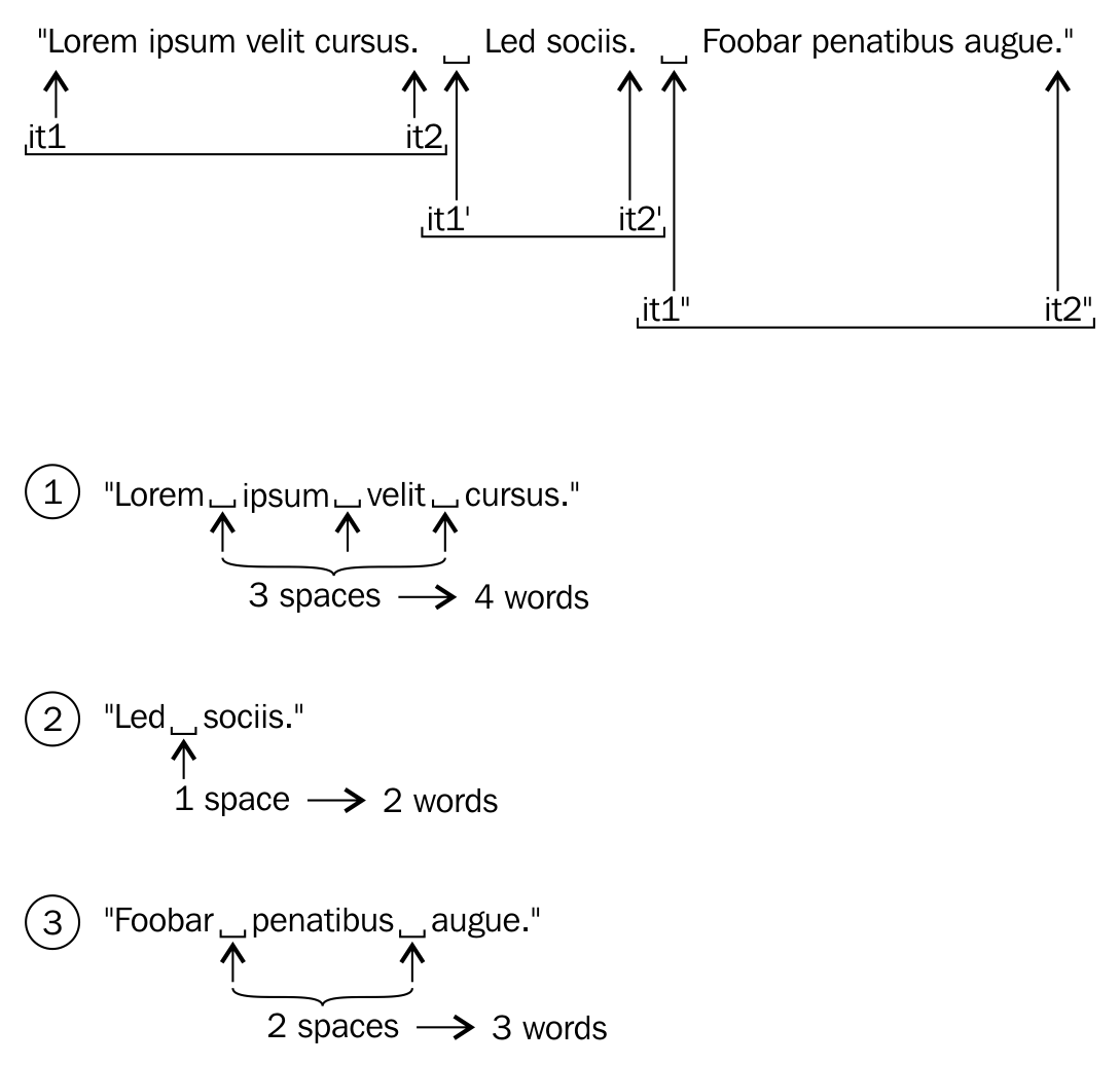
The it1 and it2 are always moved forward through the string together. This way they always point to the beginning and end of one sentence. The std::find algorithm helps us a lot in that regard because it works like "start at the current position and then return an iterator to the next dot character. If there is none, return the end iterator."
After we extract a sentence string, we determine how many words it contains, so we can insert it into the multimap. We are using the number of words as the key for the map nodes, and the string itself as the payload object associated with it. There can easily be multiple sentences which have the same length. This would render us unable to insert them all into one std::map. But since we use std::multimap, this is no problem, because it can easily handle multiple keys of the same value. It will keep them all ordered in line, which is what we need to enumerate all sentences by their length and output them to the user.
After having read the whole file into one large string, we iterate through the string and create copies of every sentence again. This is not necessary, as we also could have used std::string_view, which will be covered later in this book.
Another way to iteratively get the strings between two consecutive dots is std::regex_iterator, which will also be covered in a later chapter of this book.
The std::priority_queue is another container adapter class, such as std::stack. It is a wrapper around another data structure (std::vector by default) and provides a queue-like interface for it. This means that items can stepwise be pushed into it, and stepwise be popped out of it again. What is pushed into it first, will be popped out of it first. This is usually also abbreviated as a first in, first out (FIFO) queue. This is the opposite of a stack, where the last item pushed onto it is popped out of it first.
While we just described the behavior of std::queue, this section shows how std::priority_queue works. That adapter is special, as it does not only take FIFO characteristics into account but also mixes it with priorities. This means that the FIFO principle is kind of broken down into sub-FIFO queues, which are ordered by the priorities their items have.
In this section, we will set up a cheap to-do list organizing structure. We do not parse user input in order to keep this program short and concentrate on std::priority_queue. So we're just filling an unordered list of to-do items with priorities and descriptions into a priority queue, and then read them out like from a FIFO queue data structure, but grouped by the priorities of the individual items.
#include <iostream>
#include <queue>
#include <tuple>
#include <string>
int main()
{
using item_type = std::pair<int, std::string>;
std::priority_queue<item_type> q;
std::initializer_list<item_type> il {
{1, "dishes"},
{0, "watch tv"},
{2, "do homework"},
{0, "read comics"},
};
for (const auto &p : il) {
q.push(p);
}
while(!q.empty()) {
std::cout << q.top().first << ": " << q.top().second << 'n';
q.pop();
}
std::cout << 'n';
}
$ ./main
2: do homework
1: dishes
0: watch tv
0: read comics
The std::priority list is very easy to use. We have only used three functions:
But how did the item ordering work? We grouped a priority integer and a to-do item description string into an std::pair and got automatic ordering. If we have an std::pair<int, std::string> instance p, we can write p.first to access the integer part, and p.second to access the string part. We did that in the loop which prints out all to-do items.
But how did the priority queue infer that {2, "do homework"} is more important than {0, "watch tv"}, without us telling it to compare the numeric part?
The comparison operator < handles different cases. Let's assume we compare left < right and left and right are pairs.
This way, we can order the items as we need. The only important thing is that the priority is the first member of the pair, and the description is the second member of the pair. Otherwise, std::priority_queue would order the items in a way where it looks like the alphabetic order of the items is more important than their priorities. (In that case, watch TV would be suggested as the first thing to do, and do homework some time later. That would at least be great for those of us who are lazy!)
We cover the following recipes in this chapter:
Iterators are an extremely important concept in C++. The STL aims to be as flexible and generic as possible, and iterators are a great help in that regard. Unfortunately, they are sometimes a bit tedious to use, which is why many novices avoid them and fall back to C-Style C++. A programmer who avoids iterators basically waives half the potential of the STL. This chapter deals with iterators and quickly casts some light on how they work. That very quick introduction is probably not enough, but the recipes are really here to give a good feeling for iterator internals.
Most container classes, but also old-school C-style arrays, in one or the other way, contain a range of data items. A lot of day-to-day tasks that process a lot of data items do not care how to get at that data. However, if we regard, for example, an array of integers and a linked list of integers and want to calculate the sum of all the items of both the structures, we would end up with two different algorithms, which could look like the following:
int sum {0};
for (size_t i {0}; i < array_size; ++i) { sum += array[i]; }
int sum {0};
while (list_node != nullptr) {
sum += list_node->value; list_node = list_node->next;
}
Both of them are about summing up integers, but how large is the percentage of characters that we typed, which is directly related to the actual summing up task? And does one of them work with a third kind of data structure, let's say std::map, or do we have to implement another version of it? Without iterators, this would lead us into ridiculous directions.
Only with the help of iterators is it possible to implement this in a generic form:
int sum {0};
for (int i : array_or_vector_or_map_or_list) { sum += i; }
This pretty and short, so-called, range-based for loop has been in existence since C++11. It is just a syntax sugar, which expands to something similar to the following code:
{
auto && __range = array_or_vector_or_map_or_list ;
auto __begin = std::begin(__range);
auto __end = std::end(__range);
for ( ; __begin != __end; ++__begin) {
int i = *__begin;
sum += i;
}
}
This is an old hat for everyone who has worked with iterators already and looks completely magic for everyone who didn't. Imagine our vector of integers looks like the following:
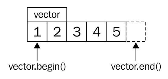
The std::begin(vector) command is the same as vector.begin() and returns us an iterator that points to the first item (the 1). std::end(vector) is the same as vector.end() and returns an iterator that points at one item past the last item (past the 5).
In every iteration, the loop checks if the begin iterator is non-equal to the end iterator. If so, it will dereference the begin iterator and thus access the integer value it points to. Then, it increments the iterator, repeats the comparison against the end iterator, and so on. In that moment, it helps to read the loop code again while imagining that the iterators are plain C-style pointers. In fact, plain C-style pointers are also a valid kind of iterators.
There are multiple categories of iterators, and they have different limitations. They are not too hard to memorize, just remember that the capabilities one category requires are inherited from the next powerful category. The whole point of iterator categories is that if an algorithm knows what kind of iterator it is dealing with, it can be implemented in an optimized way. This way, the programmer can lean back and express his intent, while the compiler can choose the optimal implementation for the given task.
Let's go through them in the right order:
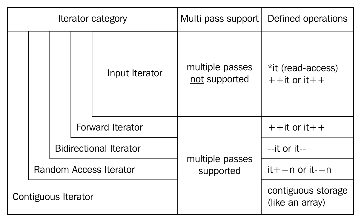
Input iterators can be dereferenced only for reading the values they point to. Once they are incremented, the last value they pointed to has been invalidated during the incrementation. This means that it is not possible to iterate over such a range multiple times. The std::istream_iterator is an example for this category.
Forward iterators are the same as input iterators, but they differ in that regard that the ranges they represent can be iterated over multiple times. The std::forward_list iterators are an example of that. Such a list can only be iterated over forward, not backward, but it can be iterated over as often as we like to.
The bidirectional iterator, as the name suggests, can be incremented and decremented, in order to iterate forward or backward. The iterators of std::list, std::set, and std::map, for example, support that.
Random access iterators allow jumping over multiple values at once, instead of single-stepping. This is the case for iterators of std::vector and std::deque.
This category specifies all of the aforementioned requirements, plus the requirement that the data that is being iterated through lies in contiguous memory, like it does in an array, or std::vector.
Output iterators are detached from the other categories. This is because an iterator can be a pure output iterator, which can only be incremented and used to write to the data it points to. If they are being read from, the value will be undefined.
If an iterator is an output iterator and one of the other categories at the same time, it is a mutable iterator. It can be read from and written to. If we obtain an iterator from a non-const container instance, it will usually be of this kind.
We already realized that iterators are, kind of, the standard interface for iterations over containers of all kinds. We just need to implement the prefix increment operator, ++, the dereference operator, *, and the object comparison operator, ==, and then we already have a primitive iterator that fits into the fancy C++11 range-based for loop.
In order to get used to this a bit more, this recipe shows how to implement an iterator that just emits a range of numbers when iterating through it. It is not backed by any container structure or anything similar. The numbers are generated ad hoc while iterating.
In this recipe, we will implement our own iterator class, and then, we will iterate through it:
#include <iostream>
class num_iterator {
int i;
public:
explicit num_iterator(int position = 0) : i{position} {}
int operator*() const { return i; }
num_iterator& operator++() {
++i;
return *this;
}
bool operator!=(const num_iterator &other) const {
return i != other.i;
}
};
class num_range {
int a;
int b;
public:
num_range(int from, int to)
: a{from}, b{to}
{}
num_iterator begin() const { return num_iterator{a}; }
num_iterator end() const { return num_iterator{b}; }
};
int main()
{
for (int i : num_range{100, 110}) {
std::cout << i << ", ";
}
std::cout << 'n';
}
100, 101, 102, 103, 104, 105, 106, 107, 108, 109,
Consider that we write the following code:
for (auto x : range) { code_block; }
The compiler will evaluate it to the following:
{
auto __begin = std::begin(range);
auto __end = std::end(range);
for ( ; __begin != __end; ++__begin) {
auto x = *__begin;
code_block
}
}
While looking at this code, it becomes obvious that the only requirements for the iterators are the following three operators:
The requirements of the range are that it has a begin and an end method, which return two iterators that denote the beginning and the end of a range.
What we did in this recipe is just fit a simple number counting algorithm into the forward iterator interface. Implementing an iterator and a range always involves this minimum amount of boilerplate code, which can be a little bit annoying on the one hand. A look at the loop that uses num_range is, on the other hand, very rewarding because it looks so perfectly simple!
Whatever own container data structure we come up with, in order to effectively mix it with all the STL goodness, we need to make them provide iterator interfaces. In the last section, we learned how to do that, but we do soon realize that some STL algorithms do not compile well with our custom iterators. Why?
The problem is that a lot of STL algorithms try to find out more about the iterators they are asked by us to deal with. Different iterator categories have different capabilities, and hence, there might be different possibilities to implement the same algorithm. For example, if we copy plain numbers from one std::vector to another, this may be implemented with a fast memcpy call. If we copy data from or to std::list, this is not possible any longer and the items have to be copied individually one by one. The implementers of the STL algorithms put a lot of thought into this kind of automatic optimization. In order to help them, we can equip our iterators with some information about them. This section shows how to achieve the same.
In this section, we will implement a primitive iterator that counts numbers and use it together with an STL algorithm, which initially does not compile with it. Then we do what's necessary to make it STL-compatible.
#include <iostream>
#include <algorithm>
class num_iterator
{
int i;
public:
explicit num_iterator(int position = 0) : i{position} {}
int operator*() const { return i; }
num_iterator& operator++() {
++i;
return *this;
}
bool operator!=(const num_iterator &other) const {
return i != other.i;
}
bool operator==(const num_iterator &other) const {
return !(*this != other);
}
};
class num_range {
int a;
int b;
public:
num_range(int from, int to)
: a{from}, b{to}
{}
num_iterator begin() const { return num_iterator{a}; }
num_iterator end() const { return num_iterator{b}; }
};
using namespace std;
int main()
{
num_range r {100, 110};
auto [min_it, max_it] (minmax_element(begin(r), end(r)));
cout << *min_it << " - " << *max_it << 'n';
}
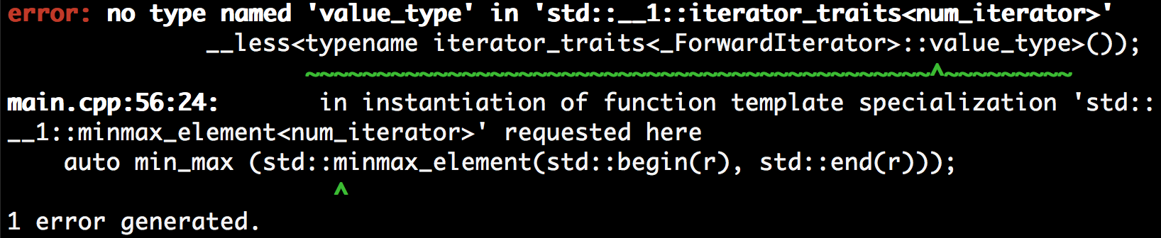
namespace std {
struct iterator_traits<num_iterator> {
using iterator_category = std::forward_iterator_tag;
using value_type = int;
using difference_type = void;
using pointer = int*;
using reference = int&;
};
}
100 - 109
Some STL algorithms need to know the characteristics of the iterator type they are used with. Some others need to know the type of items the iterators iterate over. This has different implementation reasons.
However, all STL algorithms will access this type information via std::iterator_traits<my_iterator>, assuming that the iterator type is my_iterator. This traits class contains up to five different type member definitions:
The pointer, reference, and difference_type type definitions do not make sense for our num_iterator, as it doesn't iterate over real memory values (we just return int values but they are not persistently available like in an array). Therefore it's better to not define them because if an algorithm depends on those items being referenceable in memory, it might be buggy when combined with our iterator.
Until C++17, it was encouraged to let iterator types just inherit from std::iterator<...>, which automatically populates our class with all the type definitions. This still works, but it is discouraged since C++17.
In a lot of situations, we want to fill any container with masses of data, but the data source and the container have no common interface. In such a situation, we would need to write our own hand-crafted algorithms that just deal with the question of how to shove data from the source to the sink. Usually, this distracts us from our actual work of solving a specific problem.
Tasks where we simply transport data between conceptually different data structures can be implemented with a one-liner code, thanks to another abstraction provided by the STL: iterator adapters. This section demonstrates the use of some of them in order to give a feeling how useful they are.
In this section, we use some iterator wrappers just for the sake of showing that they exist and how they can help us in everyday programming tasks.
#include <iostream>
#include <string>
#include <iterator>
#include <sstream>
#include <deque>
using namespace std;
int main()
{
istream_iterator<int> it_cin {cin};
istream_iterator<int> end_cin;
deque<int> v;
copy(it_cin, end_cin, back_inserter(v));
istringstream sstr {"123 456 789"};
auto deque_middle (next(begin(v),
static_cast<int>(v.size()) / 2));
copy(istream_iterator<int>{sstr}, {}, inserter(v, deque_middle));
initializer_list<int> il2 {-1, -2, -3};
copy(begin(il2), end(il2), front_inserter(v));
copy(begin(v), end(v), ostream_iterator<int>{cout, ", "});
cout << 'n';
}
$ echo "1 2 3 4 5" | ./main
-3, -2, -1, 1, 2, 123, 456, 789, 3, 4, 5,
We used a lot of different iterator adapters in this section. They all have one thing in common, which is they wrap an object into an iterator that is not an iterator itself.
The back_insert_iterator can be wrapped around std::vector, std::deque, std::list, and so on. It will call the container's push_back method, which inserts the new item past the existing items. If the container instance is not large enough, it will be grown automatically.
The front_insert_iterator does exactly the same thing as back_insert_iterator, but it calls the container's push_front method, which inserts the new item before all the existing items. Note that for a container like std::vector, this means that all the existing items need to be moved one slot further in order to leave space for the new item at the front.
This iterator adapter is similar to the other inserters, but is able to insert new items between existing ones. The std::inserter helper function which constructs such a wrapper takes two arguments. The first argument is the container and the second argument is an iterator that points to the position where new items shall be inserted.
The istream_iterator is another very handy adapter. It can be used with any std::istream object (which can be the standard input or files for example) and will try to parse the input from that stream object according to the template parameter it was instantiated with. In this section, we used std::istream_iterator<int>(std::cin), which pulls integers out of the standard input for us.
The special thing about streams is that we often cannot know in advance how long the stream is. That leaves the question, where will the end iterator point to if we do not know where the stream's end is? The way this works is that the iterator knows when it reaches the end of the stream. When it is compared to the end iterator, it will effectively not really compare itself with the end iterator but return if the stream has any tokens left. That's why the end iterator constructor does not take any arguments.
The ostream_iterator is the same thing as the istream_iterator, but it works the other way around: It doesn't take tokens from an input stream--it pushes tokens into an output stream. Another difference to istream_iterator is that its constructor takes a second argument, which is a string that shall be pushed into the output stream after each item. That is useful because this way we can print a separating ", " or a new line after each item.
Iterators usually iterate by moving their position from one item of a container to another. But they do not necessarily need to iterate over data structures at all. Iterators can also be used to implement algorithms, in which case, they would calculate the next value when they are incremented (++it) and return that value when they are dereferenced (*it).
In this section, we demonstrate this by implementing the Fibonacci function in form of an iterator. The Fibonacci function is recursively defined like this: F(n) = F(n - 1) + F(n - 2). It starts with the beginning values of F(0) = 0 and F(1) = 1. This leads to the following number sequence:
If we implement this in the form of a callable function that returns the Fibonacci value for any number, n, we will end up with a recursive self-calling function, or a loop implementation. This is fine, but what if we write some program where have to consume Fibonacci numbers in some pattern, one after the other? We would have two possibilities--either we recalculate all the recursive calls for every new Fibonacci number, which is a waste of computing time, or we save the last two Fibonacci numbers as temporary variables and use them to calculate the next. In the latter case, we reimplemented the Fibonacci algorithm loop implementation. It seems that we would end up mixing Fibonacci code with our actual code, which solves a different problem:
size_t a {0};
size_t b {1};
for (size_t i {0}; i < N; ++i) {
const size_t old_b {b};
b += a;
a = old_b;
// do something with b, which is the current fibonacci number
}
Iterators are an interesting way out of this. How about wrapping the steps that we do in the loop-based iterative Fibonacci implementation in the prefix increment ++ operator implementation of a Fibonacci value iterator? This is pretty easy, as this section demonstrates.
In this section, we concentrate on implementing an iterator that generates numbers from the Fibonacci number sequence while iterating over it.
#include <iostream>
class fibit
{
size_t i {0};
size_t a {0};
size_t b {1};
public:
fibit() = default;
explicit fibit(size_t i_)
: i{i_}
{}
size_t operator*() const { return b; }
fibit& operator++() {
const size_t old_b {b};
b += a;
a = old_b;
++i;
return *this;
}
bool operator!=(const fibit &o) const { return i != o.i; }
};
class fib_range
{
size_t end_n;
public:
fib_range(size_t end_n_)
: end_n{end_n_}
{}
fibit begin() const { return fibit{}; }
fibit end() const { return fibit{end_n}; }
};
int main()
{
for (size_t i : fib_range(10)) {
std::cout << i << ", ";
}
std::cout << 'n';
}
1, 1, 2, 3, 5, 8, 13, 21, 34, 55,
In order to use this iterator with the STL, it must support the std::iterator_traits class. To see how to do that, have a look at the other recipe, which deals with exactly that matter: Making your own iterators compatible with STL iterator categories.
In order to keep the example simple, we did not do anything about this, but if we do publish the Fibonacci iterator as a library, it would become apparent that it has a usability flaw--a fibit instance that was created with a constructor parameter will only be used as an end iterator because it does not contain valid Fibonacci values. Our tiny library does not enforce such usage. There are different possibilities to fix it:
Sometimes, it is valuable to iterate over a range the other way around, not forward but backward. The range-based for loop, as well as all STL algorithms usually iterate over the given ranges by incrementing iterators, although iterating backward requires decrementing them. Of course, it is possible to wrap iterators into a layer that transforms an increment call effectively into a decrement call. This sounds like a lot of boilerplate code for every type on which we would like to support that.
The STL provides a helpful reverse-iterator adapter, which helps us set up such iterators.
In this section, we will use reverse iterators in different ways, just to show how they are used:
#include <iostream>
#include <list>
#include <iterator>
using namespace std;
int main()
{
list<int> l {1, 2, 3, 4, 5};
copy(l.rbegin(), l.rend(), ostream_iterator<int>{cout, ", "});
cout << 'n';
copy(make_reverse_iterator(end(l)),
make_reverse_iterator(begin(l)),
ostream_iterator<int>{cout, ", "});
cout << 'n';
}
5, 4, 3, 2, 1,
5, 4, 3, 2, 1,
In order to be able to transform a normal iterator into a reverse iterator, it must at least have support for bidirectional iteration. This requirement is fulfilled by any iterator of the bidirectional category or higher.
A reverse iterator kind of contains a normal iterator and mimics its interface completely, but it rewires the increment operation to a decrement operation.
The next detail is about the begin and end iterator positions. Let's have a look at the following diagram, which shows a standard numeric sequence kept in an iterable range. If the sequence goes from 1 to 5, then the begin iterator has to point to the element 1, and the end iterator must point one element past 5:
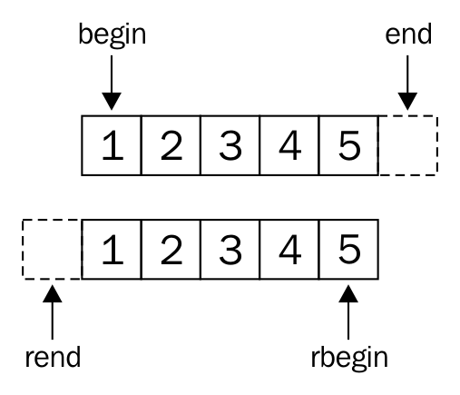
When defining reverse iterators, the rbegin iterator must point to 5, and the rend iterator must point to the element before 1. Turn the book upside down, and see that it completely makes sense.
If we want our own custom container classes to support reverse iteration, we do not need to implement all these details ourselves; we can just wrap the normal iterators into reverse iterators by using the std::make_reverse_iterator helper function, and it does all the operator rewiring and offset corrections for us.
Both STL algorithms and the range-based for loop assume that the begin and end positions of the iteration are known in advance. In some situations, however, it is hardly possible to know the end position before reaching it by iteration.
A very simple example for this is iterating over plain C-Style strings, the length of which is not known before runtime. The code which iterates over such strings usually looks like this:
for (const char *c_ponter = some_c_string; *c_pointer != ''; ++c_pointer) {
const char c = *c_pointer;
// do something with c
}
The only way to put this into a range-based for loop seems to be wrapping it into an std::string, which has begin() and end() functions:
for (char c : std::string(some_c_string)) { /* do something with c */ }
However, the constructor of std::string will iterate over the whole string before our for loop can iterate over it. Since C++17, we also have std::string_view, but its constructor will also iterate through the string once. This is not worth the real hassle for short strings, but this is also only an example for a problem class, which can be worth the hassle in other situations. The std::istream_iterator also has to deal with this when it captures input from std::cin, as its end iterator cannot realistically point to the end of the user input while the user is still typing keys.
C++17 comes with the great news that it does not constrain begin and end iterators to be of the same type. This section demonstrates how to put this little rule change to great use.
In this section, we will build an iterator together with a range class, which enables us to iterate over a string with unknown length, without finding the end position in advance.
#include <iostream>
class cstring_iterator_sentinel {};
class cstring_iterator {
const char *s {nullptr};
public:
explicit cstring_iterator(const char *str)
: s{str}
{}
char operator*() const { return *s; }
cstring_iterator& operator++() {
++s;
return *this;
}
bool operator!=(const cstring_iterator_sentinel) const {
return s != nullptr && *s != '';
}
};
class cstring_range {
const char *s {nullptr};
public:
cstring_range(const char *str)
: s{str}
{}
cstring_iterator begin() const {
return cstring_iterator{s};
}
cstring_iterator_sentinel end() const {
return {};
}
};
int main(int argc, char *argv[])
{
if (argc < 2) {
std::cout << "Please provide one parameter.n";
return 1;
}
for (char c : cstring_range(argv[1])) {
std::cout << c;
}
std::cout << 'n';
}
$ ./main "abcdef"
abcdef
That the loop prints what we just entered is not a surprise, as this is just quite a micro-example for the implementation of a sentinel-based iterator range. This iteration termination method will help you in implementing your own iterators wherever you run into a situation where the comparison with an end position approach is not helpful.
No matter how useful iterators are, and what generic interface they represent, iterators can easily be misused, just as pointers. When dealing with pointers, code must be written in a way that it never dereferences them when they point to invalid memory locations. Same applies to iterators, but there are a lot of rules that state when an iterator is valid and when it is invalidated. Those can easily be learned by studying the STL documentation a bit, but it will still always be possible to write buggy code.
In the best case, such buggy code blows up in front of the developer while it is being tested, and not on the client's machine. However, in many cases, the code just silently seems to work, although it dereferences dangling pointers, iterators, and so on. In such cases, we want to be eagerly alarmed if we produce code showing undefined behavior.
Fortunately, there's help! The GNU STL implementation has a debug mode, and the GNU C++ compiler as well as the LLVM clang C++ compiler both support additional libraries that can be used to produce extra-sensitive and verbose binaries for us, which immediately blow up on a large variety of bugs. This is easy to use and super useful, as we will demonstrate in this section. The Microsoft Visual C++ standard library also provides a possibility to activate additional checks.
In this section, we'll write a program that deliberately accesses an invalidated iterator:
#include <iostream>
#include <vector>
int main()
{
std::vector<int> v {1, 2, 3};
v.shrink_to_fit();
const auto it (std::begin(v));
std::cout << *it << 'n';
v.push_back(123);
std::cout << *it << 'n'; // bad bad bad!
}

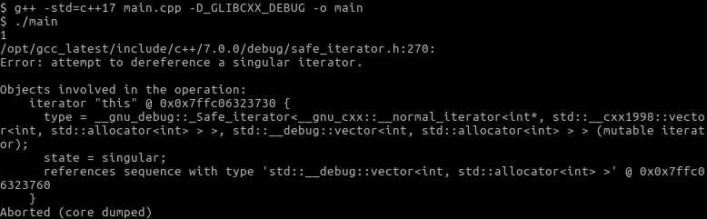
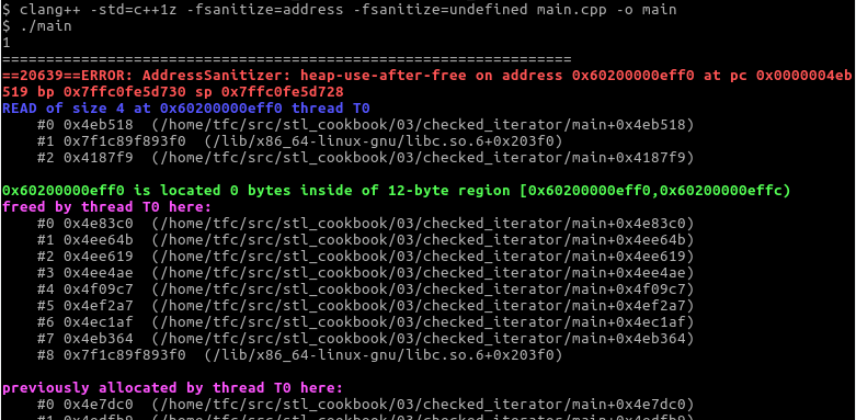
Wow, this is a very precise description of what went wrong. The screenshot would have spanned multiple pages of this book if it had not been truncated. Note that this is not a clang-only feature, as it also works with GCC.
As we have seen, we did not need to change anything in the code in order to get this kind of tripwire feature for buggy code. It basically came for free, just by appending some compiler flags to the command line when compiling the program.
This feature is implemented by sanitizers. A sanitizer usually consists of an additional compiler module and a runtime library. When sanitizers are activated, the compiler will add additional information and code to the binary, which results from our program. At runtime, the sanitizer libraries that are then linked into the program binary can, for example, replace the malloc and free functions in order to analyze how the program deals with the memory it acquires.
Sanitizers can detect different kinds of bugs. Just to list a few valuable examples:
There are many more such bugs that sanitizers can detect.
It is not feasible to always activate all available sanitizers because they make the program slower. However, it is good style to always activate sanitizers in your unit tests and integration tests.
There are a lot of different sanitizers for different bug categories, and they are all still under development. We can and should inform ourselves on the internet about how we can improve our test binaries. The GCC and LLVM project homepages list their sanitizing capabilities in their online documentation pages:
Thorough testing with sanitizers is something that every programmer should be aware of and should always be doing. Unfortunately, this is not the case in alarmingly many companies, although buggy code is the most important entry point for all the malware and computer viruses out there.
When you get a new job as a software developer, check if your team really uses all the sanitizing possibilities there are. If not, you have the unique chance to fix important and sneaky bugs on your first day at work!
Different programming languages lead to different programming styles. This is, because there are different ways to express things, and they are differing in their elegance for each use case. That is no surprise because every language was designed with specific objectives.
A very special kind of programming style is purely functional programming. It is magically different from the imperative programming which C or C++ programmers are used to. While this style is very different, it enables extremely elegant code in many situations.
One example of this elegance is the implementation of formulas, such as the mathematical dot product. Given two mathematical vectors, applying the dot product to them means pairwise multiplying of the numbers at the same positions in the vector and then summing up all of those multiplied values. The dot product of two vectors (a, b, c) * (d, e, f) is (a * e + b * e + c * f). Of course, we can do that with C and C++, too. It could look like the following:
std::vector<double> a {1.0, 2.0, 3.0};
std::vector<double> b {4.0, 5.0, 6.0};
double sum {0};
for (size_t i {0}; i < a.size(); ++i) {
sum += a[i] * b[i];
}
// sum = 32.0
How does it look like in those languages that can be considered more elegant?
Haskell is a purely functional language, and this is how you can calculate the dot product of two vectors with a magical one-liner:
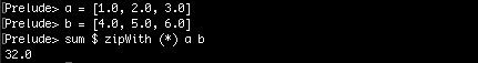
Python is not a purely functional language, but it supports similar patterns to some extent, as seen in the next example:
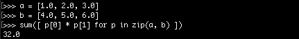
The STL provides a specific algorithm called std::inner_product, which solves this specific problem in one line, too. But the point is that in many other languages, such code can be written on the fly in only one line without specific library functions that support that exact purpose.
Without delving into the explanations of such foreign syntax, an important commonality in both examples is the magical zip function. What does it do? It takes the two vectors a and b and transforms them to a mixed vector. Example: [a1, a2, a3] and [b1, b2, b3] result in [ (a1, b1), (a2, b2), (a3, b3) ] when they are zipped together. Have a close look at it; it's really similar to how zip fasteners work!
The relevant point is that it is now possible to iterate over one combined range where pairwise multiplications can be done and then summed up to an accumulator variable. Exactly the same happens in the Haskell and Python examples, without adding any loop or index variable noise.
It will not be possible to make the C++ code exactly as elegant and generic as in Haskell or Python, but this section explains how to implement similar magic using iterators, by implementing a zip iterator. The example problem of calculating the dot product of two vectors is solved more elegantly by specific libraries, which are beyond the scope of this book. However, this section tries to show how much iterator-based libraries can help in writing expressive code by providing extremely generic building blocks.
In this section, we will recreate the zip function as known from Haskell or Python. It will be hardcoded to vectors of double variables in order to not distract from iterator mechanics:
#include <iostream>
#include <vector>
#include <numeric>
class zip_iterator {
using it_type = std::vector<double>::iterator;
it_type it1;
it_type it2;
public:
zip_iterator(it_type iterator1, it_type iterator2)
: it1{iterator1}, it2{iterator2}
{}
zip_iterator& operator++() {
++it1;
++it2;
return *this;
}
bool operator!=(const zip_iterator& o) const {
return it1 != o.it1 && it2 != o.it2;
}
bool operator==(const zip_iterator& o) const {
return !operator!=(o);
}
std::pair<double, double> operator*() const {
return {*it1, *it2};
}
};
namespace std {
template <>
struct iterator_traits<zip_iterator> {
using iterator_category = std::forward_iterator_tag;
using value_type = std::pair<double, double>;
using difference_type = long int;
};
}
class zipper {
using vec_type = std::vector<double>;
vec_type &vec1;
vec_type &vec2;
public:
zipper(vec_type &va, vec_type &vb)
: vec1{va}, vec2{vb}
{}
zip_iterator begin() const {
return {std::begin(vec1), std::begin(vec2)};
}
zip_iterator end() const {
return {std::end(vec1), std::end(vec2)};
}
};
int main()
{
using namespace std;
vector<double> a {1.0, 2.0, 3.0};
vector<double> b {4.0, 5.0, 6.0};
zipper zipped {a, b};
const auto add_product ([](double sum, const auto &p) {
return sum + p.first * p.second;
});
const auto dot_product (accumulate(
begin(zipped), end(zipped), 0.0, add_product));
cout << dot_product << 'n';
}
32
OK, that was a lot of work for a little bit of syntax sugar, and it's still not as elegant as Haskell code can be without any effort. A big flaw is the hardcoded nature of our little zip iterator--it only works on the std::vector ranges of double variables. With a bit of template code and some type traits, the zipper can be made more generic. This way, it could combine lists and vectors, or deques and maps, even if these are specialized on completely different container item types.
The amount of work and thought needed in order to really and correctly make such classes generic is not to be underestimated. Luckily, such libraries do already exist. One popular non-STL library is the Boost zip_iterator. It is very generic and easy to use.
By the way, if you came here to see the most elegant way to do a dot product in C++, and don't really care about the concept of zip-iterators, you should have a look at std::valarray. See for yourself:
#include <iostream>
#include <valarray>
int main()
{
std::valarray<double> a {1.0, 2.0, 3.0};
std::valarray<double> b {4.0, 5.0, 6.0};
std::cout << (a * b).sum() << 'n';
}
There is a very, very interesting C++ library, which supports zippers and all other kinds of magic iterator adapters, filters, and so on: the ranges library. It is inspired by the Boost ranges library, and for some time, it looked like it would find its way into C++17, but unfortunately, we will have to wait for the next standard. The reason why this is so unfortunate is that it will vigorously improve the possibilities of writing expressive and fast code in C++ by composing complex functionality from generic and simple blocks of code.
There are some very simple examples in its documentation:
const int sum = accumulate(view::ints(1)
| view::transform([](int i){return i*i;})
| view::take(10), 0);
std::vector<int> v {1,2,3,4,5,6,7,8,9,10};
auto rng = v | view::remove_if([](int i){return i % 2 == 1;})
| view::transform([](int i){return std::to_string(i);});
// rng == {"2"s,"4"s,"6"s,"8"s,"10"s};
If you are interested and can't wait for the next C++ standard, have a look at the ranges documentation at https://ericniebler.github.io/range-v3/.
We will cover the following recipes in this chapter:
One important new feature of C++11 was lambda expressions. In C++14 and C++17, the lambda expressions got some new additions, which have made them even more powerful. But first, what is a lambda expression?
Lambda expressions or lambda functions construct closures. A closure is a very generic term for unnamed objects that can be called like functions. In order to provide such a capability in C++, such an object must implement the () function calling operator, with or without parameters. Constructing such an object without lambda expressions before C++11 could still look like the following:
#include <iostream>
#include <string>
int main() {
struct name_greeter {
std::string name;
void operator()() {
std::cout << "Hello, " << name << 'n';
}
};
name_greeter greet_john_doe {"John Doe"};
greet_john_doe();
}
Instances of the name_greeter struct obviously carry a string with them. Note that both this structure type and instance are not unnamed but lambda expressions can be, as we will see. In terms of closures, we would say they capture a string. When the example instance is called like a function without parameters, it prints "Hello, John Doe" because we constructed it with this name.
Since C++11, it has become easier to create such closures:
#include <iostream>
int main() {
auto greet_john_doe ([] {
std::cout << "Hello, John Doen";
});
greet_john_doe();
}
That's it. The whole struct, name_greeter, is replaced by a little [] { /* do something */ } construct, which might look a bit like magic at first, but the first section of this chapter will explain it thoroughly in all the possible variants.
Lambda expressions are of a great help to make code generic and tidy. They can be used as parameters for very generic algorithms in order to specialize what those do when processing specific user-defined types. They can also be used to wrap work packages together with data in order to be run in threads or just to save work and postpone the actual execution. Since C++11 came out, more and more libraries work with lambda expressions because they became a very natural thing in C++. Another use case is metaprogramming, because lambda expressions can also be evaluated at compile time. However, we are not going much into that direction, as this would quickly blast the scope of this book.
This chapter does heavily rely on some functional programming patterns, which might look weird to novices or programmers who are already experienced but not with such patterns. If you see lambda expressions in the coming recipes that return lambda expressions, which again return lambda expressions, please don't feel frustrated or confused too quickly. We are pushing the boundaries a bit in order to prepare ourselves for modern C++, where functional programming patterns occur with increasing regularity. If some code in the following recipes looks a bit too complex, take your time to understand it. Once you got through this, complex lambda expressions in real projects in the wild will not confuse you any longer.
With lambda expressions, we can encapsulate code in order to call it later, and that also might be somewhere else because we can copy them around. We can also just encapsulate code to call it multiple times with slightly different parameters without having to implement a whole new function class for that task.
The syntax of lambda expressions was really new in C++11, and it has slightly evolved with the next two standard versions until C++17. In this section, we will see what lambda expressions can look like and what they mean.
We are going to write a little program in which we play with lambda expressions in order to get a feeling for them:
#include <iostream>
#include <string>
int main()
{
auto just_one ( [](){ return 1; } );
auto just_two ( [] { return 2; } );
std::cout << just_one() << ", " << just_two() << 'n';
auto plus ( [](auto l, auto r) { return l + r; } );
std::cout << plus(1, 2) << 'n';
std::cout << plus(std::string{"a"}, "b") << 'n';
std::cout
<< [](auto l, auto r){ return l + r; }(1, 2)
<< 'n';
auto counter (
[count = 0] () mutable { return ++count; }
);
for (size_t i {0}; i < 5; ++i) {
std::cout << counter() << ", ";
}
std::cout << 'n';
int a {0};
auto incrementer ( [&a] { ++a; } );
incrementer();
incrementer();
incrementer();
std::cout
<< "Value of 'a' after 3 incrementer() calls: "
<< a << 'n';
auto plus_ten ( [=] (int x) { return plus(10, x); } );
std::cout << plus_ten(5) << 'n';
}
1, 2
3
ab
3
1, 2, 3, 4, 5,
Value of a after 3 incrementer() calls: 3
15
What we just did was not overly complicated--we added numbers, and incremented and printed them. We even concatenated strings with a function object, which was implemented to add up numbers. But for anyone who didn't know lambda expression syntax yet, it might have looked confusing.
So, let's first have a look at all the lambda expression peculiarities:
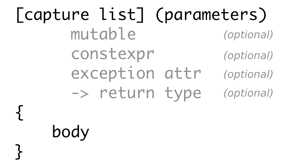
We can usually omit most of this, which spares us some typing, in the average case. The shortest lambda expression possible is []{}. It accepts no parameters, captures nothing, and essentially does nothing.
So what does the rest mean?
Specifies if and what we capture. There are several forms to do so. There are two lazy variants:
Of course, we can set the capturing settings for every variable individually. Writing [a, &b] () {...} means, that we capture the variable a by value, and b by reference. This is more typing work, but it's generally safer to be that verbose because we cannot accidentally capture something we don't want to capture from outside.
In the recipe, we defined a lambda expression as such: [count=0] () {...}. In this special case, we did not capture any variable from outside, but we defined a new one called count. Its type is deduced from the value we initialized it with, namely 0, so it's an int.
It is also possible to capture some variables by value and some, by reference, as in:
If the function object should be able to modify the variables it captures by copy ([=]), it must be defined mutable. This includes calling non-const methods of captured objects.
If we mark the lambda expression explicitly as constexpr, the compiler will error out if it does not satisfy the criteria of constexpr functions. The advantage of constexpr functions and lambda expressions is that the compiler can evaluate their result at compile time if they are called with compile-time constant parameters. This leads to less code in the binary later.
If we do not explicitly declare the lambda expression to be constexpr but it fits the requirements for that, it will be implicitly constexpr anyway. If we want a lambda expression to be constexpr, it helps to be explicit because the compiler will then help us by erroring out if we did it wrong.
This is the place to specify if the function object can throw exceptions when it's called and runs into an error case.
If we want to have ultimate control over the return type, we may not want the compiler to deduce it for us automatically. In such a case, we can just write [] () -> Foo {}, which tells the compiler that we will really always return the Foo type.
Let's say we want to write an observer function for some kind of value, which might change sometimes, which then notifies other objects; like a gas pressure indicator, or a stock price, or something similar. Whenever the value changes, a list of observer objects should be called, which then react their way.
In order to implement this, we could store a range of observer function objects in a vector, which all accept an int variable as the parameter, which represents the observed value. We do not know what these function objects do in particular when they are called with the new value, but we also don't care.
Of what type will that vector of function objects be? The std::vector<void (*)(int)> type would be correct if we were capturing pointers to functions with signatures such as void f(int);. This would indeed also work with any lambda expression that does not capture any variables, such as [](int x) {...}. But a lambda expression that captures something is actually a completely different type compared with a normal function because it's not just a function pointer. It is an object that couples a certain amount of data with a function! Think of pre-C++11 times, when there were no lambdas. Classes and structs are the natural way of coupling data with functions, and if you change the data member types of a class, you get a completely different class type. It's just natural that a vector can't store completely different types using the same type name.
Telling the user that it's only possible to save observer function objects that do not capture anything is bad because it limits the number of use cases very much. How can we allow the user to store any kind of function object, only constraining to the call interface, which takes a specific set of parameters that represent the value that shall be observed?
This section shows how to solve this problem using std::function, which can act as a polymorphic wrapper around any lambda expression, no matter if and what it captures.
In this section, we are going to create several lambda expressions that are completely different in regard to the variable types they capture but have the same function call signature in common. These will be saved in one vector using std::function:
#include <iostream>
#include <deque>
#include <list>
#include <vector>
#include <functional>
static auto consumer (auto &container){
return [&] (auto value) {
container.push_back(value);
};
}
static void print (const auto &c)
{
for (auto i : c) {
std::cout << i << ", ";
}
std::cout << 'n';
}
int main()
{
std::deque<int> d;
std::list<int> l;
std::vector<int> v;
const std::vector<std::function<void(int)>> consumers
{consumer(d), consumer(l), consumer(v)};
for (size_t i {0}; i < 10; ++i) {
for (auto &&consume : consumers) {
consume(i);
}
}
print(d);
print(l);
print(v);
}
$ ./std_function
0, 1, 2, 3, 4, 5, 6, 7, 8, 9,
0, 1, 2, 3, 4, 5, 6, 7, 8, 9,
0, 1, 2, 3, 4, 5, 6, 7, 8, 9,
The complicated part of this recipe is the following line:
const std::vector<std::function<void(int)>> consumers
{consumer(d), consumer(l), consumer(v)};
The objects d, l, and v are each wrapped into a consumer(...) call. This call returns function objects, which then each capture references to one of d, l, and v. Although these function objects all accept int values as parameters, the fact that they capture completely different variables also makes them completely different types. This is like trying to stuff variables of type A, B, and C into a vector, although these types have nothing in common.
In order to fix this, we need to find a common type, which can store very different function objects, that is, std::function. An std::function<void(int)> object can store any function object or traditional function, which accepts an integer parameter and returns nothing. It decouples its type from the underlying function object type, using polymorphy. Consider we write something like this:
std::function<void(int)> f (
[&vector](int x) { vector.push_back(x); });
Here, the function object which is constructed from the lambda expression is wrapped into an std::function object, and whenever we call f(123), this leads to a virtual function call, which is redirected to the actual function object inside it.
While storing function objects, std::function instances apply some intelligence. If we capture more and more variables in a lambda expression, it must grow larger. If its size is not too large, std::function can store it within itself. If the size of the stored function object is too large, std::function will allocate a chunk of memory on the heap and then store the large function object there. This does not affect the functionality of our code, but we should know about this because this can impact the performance of our code.
A lot of tasks are not really worthy of being implemented in completely custom code. Let's, for example, have a look on how a programmer might solve the task of finding out how many unique words a text contains with the programming language Haskell. The first line defines a function unique_words and the second one demonstrates its use with an example string:
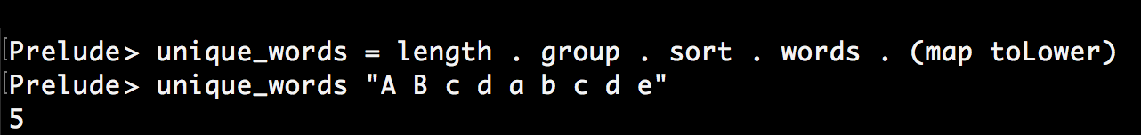
Wow, that is short! Without explaining Haskell syntax too much, let's see what the code does. It defines the function called unique_words, which applies a series of functions to its input. It first maps all the characters from the input to lowercase with map toLower. This way, words like FOO and foo can be regarded as the same word. Then, the words function splits a sentence into individual words, as from "foo bar baz" to ["foo", "bar", "baz"]. Next step is sorting the new list of words. This way, a word sequence such as ["a", "b", "a"] becomes ["a", "a", "b"]. Now, the group function takes over. It groups consecutive equal words into grouped lists, so ["a", "a", "b"] becomes [ ["a", "a"], ["b"] ]. The job is now nearly done, as we now only need to count how many groups of equal words we got, which is exactly what the length function does.
This is a wonderful style of programming, as we can read what happens from right to left because we are just, kind of, describing a transformation pipeline. We don't need to care how the individual pieces are implemented (unless it turns out that they are slow or buggy).
However, we are not here to praise Haskell but to improve our C++ skills. It is possible to work like this in C++ too. We will not completely reach the elegance of the Haskell example but we still have the fastest programming language there is. This example explains how to imitate function concatenation in C++ with lambda expressions.
In this section, we define some simple toy function objects and concatenate them, so we get a single function that applies the simple toy functions after each other to the input we give it. In order to do so, we write our own concatenation helper function:
#include <iostream>
#include <functional>
template <typename T, typename ...Ts>
auto concat(T t, Ts ...ts)
{
if constexpr (sizeof...(ts) > 0) {
return [=](auto ...parameters) {
return t(concat(ts...)(parameters...));
};
}
else {
return t;
}
}
int main()
{
auto twice ([] (int i) { return i * 2; });
auto thrice ([] (int i) { return i * 3; });
auto combined (
concat(twice, thrice, std::plus<int>{})
);
std::cout << combined(2, 3) << 'n';
}
$ ./concatenation
30
The complicated thing in this section is the concat function. It looks horribly complicated because it unpacks the parameter pack ts into another lambda expression, which recursively calls concat again, with less parameters:
template <typename T, typename ...Ts>
auto concat(T t, Ts ...ts)
{
if constexpr (sizeof...(ts) > 0) {
return [=](auto ...parameters) {
return t(concat(ts...)(parameters...));
};
} else {
return [=](auto ...parameters) {
return t(parameters...);
};
}
}
Let's write a simpler version, which concatenates exactly three functions:
template <typename F, typename G, typename H>
auto concat(F f, G g, H h)
{
return [=](auto ... params) {
return f( g( h( params... ) ) );
};
}
This already looks similar, but less complicated. We return a lambda expression, which captures f, g, and h. This lambda expression arbitrarily accepts many parameters and just forwards them to a call chain of f, g, and h. When we write auto combined (concat(f, g, h)), and later call that function object with two parameters, such as combined(2, 3), then the 2, 3 are represented by the params pack from the preceding concat function.
Looking at the much more complex, generic concat function again; the only thing we do really differently is the f ( g( h( params... ) ) ) concatenation. Instead, we write f( concat(g, h) )(params...), which evaluates to f( g( concat(h) ) )(params...) in the next recursive call, which then finally results in f( g( h( params... ) ) ).
When filtering data with generic code, we end up defining predicates, which tell what data we want, and what data we do not want. Sometimes predicates are the combinations of different predicates.
When filtering strings, for example, we could implement a predicate that returns true if its input string begins with "foo". Another predicate could return true if its input string ends with "bar".
Instead of writing custom predicates all the time, we can reuse predicates by combining them. If we want to filter strings that begin with "foo" and end with "bar", we can just pick our existing predicates and combine them with a logical and. In this section, we play with lambda expressions in order to find a comfortable way to do this.
We will implement very simple string filter predicates, and then we will combine them with a little helper function that does the combination for us in a generic way.
#include <iostream>
#include <functional>
#include <string>
#include <iterator>
#include <algorithm>
static bool begins_with_a (const std::string &s)
{
return s.find("a") == 0;
}
static bool ends_with_b (const std::string &s)
{
return s.rfind("b") == s.length() - 1;
}
template <typename A, typename B, typename F>
auto combine(F binary_func, A a, B b)
{
return [=](auto param) {
return binary_func(a(param), b(param));
};
}
using namespace std;
int main()
{
auto a_xxx_b (combine(
logical_and<>{},
begins_with_a, ends_with_b));
copy_if(istream_iterator<string>{cin}, {},
ostream_iterator<string>{cout, ", "},
a_xxx_b);
cout << 'n';
}
$ echo "ac cb ab axxxb" | ./combine
ab, axxxb,
The STL already provides a useful bunch of functional objects such as std::logical_and, std::logical_or, as well as many others, so we do not need to reimplement them in every project. It's a good idea to have a look at the C++ reference and explore what's there already:
http://en.cppreference.com/w/cpp/utility/functional
There are a lot of tasks, which lead to repetitive code. A lot of repetitive code can be eliminated easily using lambda expressions and a lambda expression helper that wraps such repetitive tasks is created very quickly.
In this section, we will play with lambda expressions in order to forward a single call with all its parameters to multiple receivers. This is going to happen without any data structures in between, so the compiler has a simple job to generate a binary without overhead.
We are going to write a lambda expression helper, which forwards a single call to multiple objects, and another lambda expression helper, which forwards a single call to multiple calls of other functions. In our example, we are going to use this to print a single message with different printer functions:
#include <iostream>
static auto multicall (auto ...functions)
{
return [=](auto x) {
(void)std::initializer_list<int>{
((void)functions(x), 0)...
};
};
}
static auto for_each (auto f, auto ...xs) {
(void)std::initializer_list<int>{
((void)f(xs), 0)...
};
}
static auto brace_print (char a, char b) {
return [=] (auto x) {
std::cout << a << x << b << ", ";
};
}
int main()
{
auto f (brace_print('(', ')'));
auto g (brace_print('[', ']'));
auto h (brace_print('{', '}'));
auto nl ([](auto) { std::cout << 'n'; });
auto call_fgh (multicall(f, g, h, nl));
for_each(call_fgh, 1, 2, 3, 4, 5);
}
$ ./multicaller
(1), [1], {1},
(2), [2], {2},
(3), [3], {3},
(4), [4], {4},
(5), [5], {5},
The helpers we just implemented look horribly complicated. This is because we expand parameter packs with std::initializer_list. Why did we even use that data structure? Let's have a look at for_each again:
auto for_each ([](auto f, auto ...xs) {
(void)std::initializer_list<int>{
((void)f(xs), 0)...
};
});
The heart of this function is the f(xs) expression. xs is a parameter pack, and we need to unpack it in order to get the individual values out of it and feed them to individual f calls. Unfortunately, we cannot just write f(xs)... using the ... notation, which we already know.
What we can do is constructing a list of values using std::initializer_list, which has a variadic constructor. An expression such as return std::initializer_list<int>{f(xs)...}; does the job, but it has downsides. Let's have a look at an implementation of for_each which does just this, so it looks simpler than what we have:
auto for_each ([](auto f, auto ...xs) {
return std::initializer_list<int>{f(xs)...};
});
This is easier to grasp, but its downsides are the following:
The much more complicated for_each function fixes all these problems. It does the following things to achieve that:
Putting all this together unluckily leads to an ugly construct, but it does it's work right and compiles with a whole variety of function objects, regardless of whether they return anything or what they return.
A nice detail of this technique is that the order in which the function calls are applied is guaranteed to be in a strict sequence.
Most developers who have used std::copy_if and std::transform may have asked themselves already, why there is no std::transform_if. The std::copy_if function copies items from a source range to a destination range, but skips the items that are not selected by a user-defined predicate function. The std::transform unconditionally copies all items from a source range to a destination range but transforms them in between. The transformation is provided by a user-defined function, which might do simple things, such as multiplying numbers or transforming items to completely different types.
Such functions have been there for a long time now, but there is still no std::transform_if function. In this section, we are going to implement this function. It would be easy to do this by just implementing a function that iterates over the ranges while copying all the items that are selected by a predicate function and transforming them in between. However, we'll use this occasion to delve deeper into lambda expressions.
We are going to build our own transform_if function which works by supplying std::accumulate with the right function objects:
#include <iostream>
#include <iterator>
#include <numeric>
template <typename T>
auto map(T fn)
{
return [=] (auto reduce_fn) {
return [=] (auto accum, auto input) {
return reduce_fn(accum, fn(input));
};
};
}
template <typename T>
auto filter(T predicate)
{
return [=] (auto reduce_fn) {
return [=] (auto accum, auto input) {
if (predicate(input)) {
return reduce_fn(accum, input);
} else {
return accum;
}
};
};
}
int main()
{
std::istream_iterator<int> it {std::cin};
std::istream_iterator<int> end_it;
auto even ([](int i) { return i % 2 == 0; });
auto twice ([](int i) { return i * 2; });
auto copy_and_advance ([](auto it, auto input) {
*it = input;
return ++it;
});
std::accumulate(it, end_it,
std::ostream_iterator<int>{std::cout, ", "},
filter(even)(
map(twice)(
copy_and_advance
)
));
std::cout << 'n';
}
$ echo "1 2 3 4 5 6" | ./transform_if
4, 8, 12,
This recipe looks really complicated because we are nesting lambda expressions a lot. In order to understand how this works, let's first have a look at the inner workings of std::accumulate. This is how it will look like in a typical STL implementation:
template <typename T, typename F>
T accumulate(InputIterator first, InputIterator last, T init, F f)
{
for (; first != last; ++first) {
init = f(init, *first);
}
return init;
}
The function parameter, f, does the main work here, while the loop collects its results in the user provided init variable. In a usual example case, the iterator range may represent a vector of numbers, such as 0, 1, 2, 3, 4, and the init value is 0. The f function is then just a binary function that might calculate the sum of two items using the + operator.
In this example case, the loop just sums up all the items into the init variable, such as in init = (((0 + 1) + 2) + 3) + 4. Writing it down like this makes obvious that std::accumulate is just a general folding function. Folding a range means applying a binary operation to an accumulator variable and stepwise every item contained in the range (the result of each operation is then the accumulator value for the next one). As this function is so general, we can do all kinds of things with it, just like implementing std::transform_if! The f function is then also called the reduce function.
A very direct implementation of transform_if will look as follows:
template <typename InputIterator, typename OutputIterator,
typename P, typename Transform>
OutputIterator transform_if(InputIterator first, InputIterator last,
OutputIterator out,
P predicate, Transform trans)
{
for (; first != last; ++first) {
if (predicate(*first)) {
*out = trans(*first);
++out;
}
}
return out;
}
This looks quite similar to std::accumulate, if we regard the parameter out as the init variable, and somehow get function f to substitute the if-construct and its body!
We actually did that. We constructed that if-construct and its body with the binary function object we provided as a parameter to std::accumulate:
auto copy_and_advance ([](auto it, auto input) {
*it = input;
return ++it;
});
The std::accumulate function puts the init variable into the binary function's it parameter. The second parameter is the current value from the source range per loop iteration step. We provided an output iterator as the init parameter of std::accumulate.. This way, std::accumulate does not calculate a sum, but forwards the items it iterates over to another range. This means that we just reimplemented std::copy without any predicate and transformation, yet.
The filtering using a predicate was added by us by wrapping the copy_and_advance function object into another function object, which employs a predicate function:
template <typename T>
auto filter(T predicate)
{
return [=] (auto reduce_fn) {
return [=] (auto accum, auto input) {
if (predicate(input)) {
return reduce_fn(accum, input);
} else {
return accum;
}
};
};
}
This construction does not look too simple at first but have a look at the if construct. If the predicate function returns true, it forwards the parameters to the reduce_fn function, which is copy_and_advance in our case. If the predicate returns false, the accum variable, which is the init variable of std::accumulate, is just returned without change. This implements the skipping part of a filter operation. The if construct is located within the inner lambda expression, which has the same binary function signature as the copy_and_advance function, which makes it a fitting substitute.
Now we are able to filter but are still not transforming. This is done with the map function helper:
template <typename T>
auto map(T fn)
{
return [=] (auto reduce_fn) {
return [=] (auto accum, auto input) {
return reduce_fn(accum, fn(input));
};
};
}
This code looks much easier. It again contains an inner lambda expression, which has the same signature as copy_and_advance has, so it can substitute it. The implementation just forwards the input values but transforms the right parameter of the binary function call with the fn function.
Later, when we used those helpers, we wrote the following expression:
filter(even)(
map(twice)(
copy_and_advance
)
)
The filter(even) call captures the even predicate and gives us a function, which takes a binary function in order to wrap it into another binary function, which does additional filtering. The map(twice) function does the same with the twice transformation function but wraps the binary function, copy_and_advance, into another binary function, which always transforms the right parameter.
Without any optimization, we would get a horribly complicated nested construction of functions that call functions and do only a very little amount of work in between. However, it is a very simple task for the compiler to optimize all the code. The resulting binary is as simple as if it resulted from a more direct implementation of transform_if. We pay nothing in terms of performance this way. But what we get is a very nice composability of functions because we were able to stick the even predicate together with the twice transformation function, nearly as simply as if they were lego bricks.
Lambda expressions in combination with parameter packs can be used for complex tasks. In this section, we will implement a function object that accepts an arbitrary number of input parameters and generates the cartesian product of this set with itself.
The cartesian product is a mathematical operation. It is noted as A x B, meaning the cartesian product of set A and set B. The result is another single set, which contains pairs of all item combinations of the sets A and B. The operation basically means, combine every item from A with every item from B. The following diagram illustrates the operation:
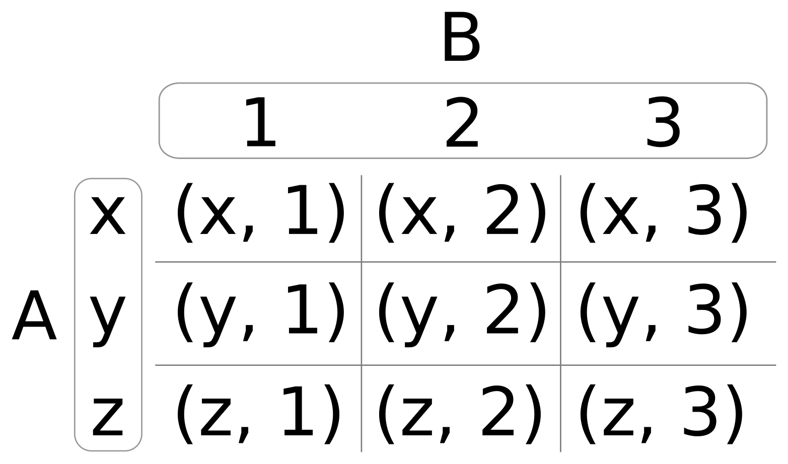
In the preceding diagram, if A = (x, y, z), and B = (1, 2, 3), then the cartesian product is (x, 1), (x, 2), (x, 3), (y, 1), (y, 2), and so on.
If we decide that A and B are the same set, say (1, 2), then the cartesian product of that is (1, 1), (1, 2), (2, 1), and (2, 2). In some cases, this might be declared redundant, because the combination of items with themselves (like in (1, 1)) or redundant combinations of (1, 2) and (2, 1) may not be needed. In such a case, the cartesian product can be filtered with a simple rule.
In this section, we will implement the cartesian product without any loops but with lambda expressions and parameter pack unpacking.
We implement a function object that accepts a function, f, and a set of parameters. The function object will create the cartesian product of the parameter set, filter out the redundant parts, and call the f function with each of them:
#include <iostream>
static void print(int x, int y)
{
std::cout << "(" << x << ", " << y << ")n";
}
int main()
{
constexpr auto call_cart (
[=](auto f, auto x, auto ...rest) constexpr {
(void)std::initializer_list<int>{
(((x < rest)
? (void)f(x, rest)
: (void)0)
,0)...
};
});
constexpr auto cartesian ([=](auto ...xs) constexpr {
return [=] (auto f) constexpr {
(void)std::initializer_list<int>{
((void)call_cart(f, xs, xs...), 0)...
};
};
});
constexpr auto print_cart (cartesian(1, 2, 3));
print_cart(print);
}
$ ./cartesian_product
(1, 2)
(1, 3)
(2, 3)
That was another really complicated-looking lambda expression construct. But as soon as we understand this thoroughly, we will not be confused by any lambda expression anytime soon!
So, let's have a detailed look at it. We should get a mental picture of what needs to happen:
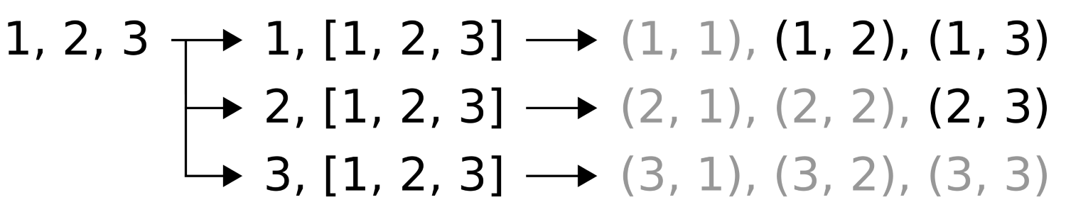
These are three steps:
Now, back to the implementation:
constexpr auto cartesian ([=](auto ...xs) constexpr {
return [=](auto f) constexpr {
(void)std::initializer_list<int>{
((void)call_cart(f, xs, xs...), 0)...
};
};
});
The inner expression, call_cart(xs, xs...), exactly represents the separation of (1, 2, 3) into those new sets, such as 1, [1, 2, 3]. The full expression, ((void)call_cart(f, xs, xs...), 0)... with the other ... outside, does this separation for every value of the set, so we also get 2, [1, 2, 3] and 3, [1, 2, 3].
Step 2 and step 3 are done by call_cart:
auto call_cart ([](auto f, auto x, auto ...rest) constexpr {
(void)std::initializer_list<int>{
(((x < rest)
? (void)f(x, rest)
: (void)0)
,0)...
};
});
Parameter x always contains the single value picked from the set, and rest contains the whole set again. Let's ignore the (x < rest) conditional at first. Here, the expression f(x, rest), together with the ... parameter pack expansion generates the function calls f(1, 1), f(1, 2), and so on, which results in the pairs being printed. This was step 2.
Step 3 is achieved by filtering out only the pairs where (x < rest) applies.
We made all lambda expressions and the variables holding them constexpr. By doing so, we can now guarantee that the compiler will evaluate their code at compile time and compile a binary that already contains all the number pairs instead of calculating them at runtime. Note that this only happens if all the function arguments we provide to a constexpr function are known at compile time already.
We will cover the following recipes in this chapter:
The STL does not only contain data structures but also algorithms, of course. While data structures help store and maintain data in different ways with different motivations and targets, algorithms apply specific transformations to the data in such data structures.
Let's have a look at a standard task, such as summing up items from a vector. This can be done easily by looping over the vector and summing up all the items into an accumulator variable called sum:
vector<int> v {100, 400, 200 /*, ... */ };
int sum {0};
for (int i : v) { sum += i; }
cout << sum << 'n';
But because this is quite a standard task, there is also an STL algorithm for this:
cout << accumulate(begin(v), end(v), 0) << 'n';
In this case, the handcrafted loop variant is not much longer, and it is also not significantly harder to read than a one-liner which says what it does: accumulate. In a lot of cases, however, it is awkward to read a 10-line code loop just to realize, "Did I just have to study the whole loop in order to understand that it does a standard task, X?", rather than seeing one line of code, which uses a standard algorithm whose name clearly states what it does, such as accumulate, copy, move, transform, or shuffle.
The basic idea is to provide a rich variety of algorithms that can be used by programmers on a daily basis in order to reduce the need to repeatedly reimplement them. This way, programmers can just use off the shelf algorithm implementations and concentrate on the new problems, instead of wasting time on problems that already have been solved by the STL. Another perspective is correctness--if a programmer implements the same thing again and again for a hundred times, there is some probability that this may introduce a slight error in one or the other attempt. This would be completely unnecessary and also very embarrassing if, for example, it is pointed out by a colleague during code review, whereas at the same time, a standard algorithm could have been used.
Another important point of STL algorithms is efficiency. Many STL algorithms provide multiple specialized implementations of the same algorithm, which do things differently, depending on the iterator type they are being used with. For example, if all the elements in a vector of integers should be zeroed, this can be done with the STL algorithm std::fill. Because the iterator of a vector can already tell the compiler that it iterates over contiguous memory, it can select the implementation of std::fill which uses the C procedure memset. If the programmer changes the container type from vector to list, then the STL algorithm cannot use memset any longer and has to iterate over the list in order to zero the items individually. In case the programmer uses memset himself, the implementation would be unnecessarily hardcoded to using vectors or arrays because most other data structures do not save their data in contiguous memory chunks. In most cases, it makes little sense to try to be smart, as the implementers of the STL may already have implemented the same ideas, which can be used for free.
Let's summarize the preceding points. Using STL algorithms is good for:
Most algorithms work on iterators. The concept of how iterators work is already explained in Chapter 20, Iterators. In this chapter, we'll concentrate on using STL algorithms for different problems in order to get a feeling of how they can be profitably put to use. Showing all STL algorithms would blow up this book to a very boring C++ reference, although there is already a C++ reference publicly available.
The best way to become an STL ninja is having the C++ reference always at hand or, at least, saved in a browser bookmark. When solving a task, every programmer should have a look at it with the question back in his mind, "Is there an STL algorithm for my problem?", before writing code himself.
A very good and complete C++ reference is available for online viewing at:
It can also be downloaded for offline viewing.
The most important STL data structures have iterator support. This means that it is at least possible to get iterators via begin() and end() functions, which point to the data structure's underlying payload data and allow to iterate over that data. The iteration always looks the same, no matter what kind of data structure is iterated over.
We can get iterators from vectors, lists, deques, maps, and so on. Using iterator adaptors, we can even get iterators as an interface to files, standard input, and standard output. Moreover, as we saw in the previous chapter, we can even wrap iterator interfaces around algorithms. Now, where we can access everything with iterators, we can combine them with STL algorithms, which accept iterators as parameters.
A really nice way to show how iterators help abstract the nature of different data structures away is the std::copy algorithm, which just copies items from one set of iterators to an output iterator. Where such algorithms are used, the nature of the underlying data structure is not really relevant any longer. In order to demonstrate this, we will play a bit with std::copy.
In this section, we will use different variants of std::copy:
#include <iostream>
#include <vector>
#include <map>
#include <string>
#include <tuple>
#include <iterator>
#include <algorithm>
using namespace std;
namespace std {
ostream& operator<<(ostream &os, const pair<int, string> &p)
{
return os << "(" << p.first << ", " << p.second << ")";
}
}int main()
{
vector<pair<int, string>> v {
{1, "one"}, {2, "two"}, {3, "three"},
{4, "four"}, {5, "five"}};
map<int, string> m;
copy_n(begin(v), 3, inserter(m, begin(m)));
auto shell_it (ostream_iterator<pair<int, string>>{cout,
", "});
copy(begin(m), end(m), shell_it);
cout << 'n';
m.clear();
move(begin(v), end(v), inserter(m, begin(m)));
copy(begin(m), end(m), shell_it);
cout << 'n';
copy(begin(v), end(v), shell_it);
cout << 'n';
}
$ ./copying_items
(1, one), (2, two), (3, three),
(1, one), (2, two), (3, three), (4, four), (5, five),
(1, ), (2, ), (3, ), (4, ), (5, ),
As std::copy is one of the simplest STL algorithms, its implementation is very short. Let's have a look at how it could be implemented:
template <typename InputIterator, typename OutputIterator>
OutputIterator copy(InputIterator it, InputIterator end_it,
OutputIterator out_it)
{
for (; it != end_it; ++it, ++out_it) {
*out_it = *it;
}
return out_it;
}
This looks exactly as one would implement the copying of items from one iterable range to the other by hand, naively. At this point, one could also ask, "So why not implementing it by hand, the loop is simple enough and I don't even need the return value?", which is, of course, a good question.
While std::copy is not the best example for making code significantly shorter, a lot of other algorithms with more complex implementations are. What is not obvious is the hidden automatic optimization of such STL algorithms. If we happen to use std::copy with data structures that store their items in contiguous memory (as std::vector and std::array do), and the items themselves are trivially copy assignable, then the compiler will select a completely different implementation (which assumes the iterator types to be pointers):
template <typename InputIterator, typename OutputIterator>
OutputIterator copy(InputIterator it, InputIterator end_it,
OutputIterator out_it)
{
const size_t num_items (distance(it, end_it));
memmove(out_it, it, num_items * sizeof(*it));
return it + num_items;
}
This is a simplified version of how the memmove variant of the std::copy algorithm can look in a typical STL implementation. It is faster than the standard loop version, and this time, it is also not as nice to read. But nevertheless, std::copy users automatically profit from it if their argument types comply with the requirements of this optimization. The compiler selects the fastest implementation possible for the chosen algorithm, while the user code nicely expresses what the algorithm does without tainting the code with too many details of the how.
STL algorithms often simply provide the best trade-off between readability and optimal implementation.
We also used std::move. It works exactly like std::copy, but it applies std::move(*it) to the source iterator in the loop in order to cast lvalues to rvalues. This makes the compiler select the move assignment operator of the target object instead of the copy assignment operator. For a lot of complex objects, this performs better but destroys the source object.
Sorting values is quite a standard task, and it can be done in various ways. Every computer science student who was tortured with having to learn a majority of existing sorting algorithms (together with their performance and stability trade-offs for exams) knows that.
Because this is a solved problem, programmers should not waste their time in solving it again, except if it is for learning purposes.
In this section, we are going to play with std::sort and std::partial_sort:
#include <iostream>
#include <algorithm>
#include <vector>
#include <iterator>
#include <random>
using namespace std;
static void print(const vector<int> &v)
{
copy(begin(v), end(v), ostream_iterator<int>{cout, ", "});
cout << 'n';
}
int main()
{
vector<int> v {1, 2, 3, 4, 5, 6, 7, 8, 9, 10};
random_device rd;
mt19937 g {rd()};
cout << is_sorted(begin(v), end(v)) << 'n';
shuffle(begin(v), end(v), g);
cout << is_sorted(begin(v), end(v)) << 'n';
print(v);
sort(begin(v), end(v));
cout << is_sorted(begin(v), end(v)) << 'n';
print(v);
shuffle(begin(v), end(v), g);
partition(begin(v), end(v), [] (int i) { return i < 5; });
print(v);
shuffle(begin(v), end(v), g);
auto middle (next(begin(v), int(v.size()) / 2));
partial_sort(begin(v), middle, end(v));
print(v);
struct mystruct {
int a;
int b;
};
vector<mystruct> mv {{5, 100}, {1, 50}, {-123, 1000},
{3, 70}, {-10, 20}};
sort(begin(mv), end(mv),
[] (const mystruct &lhs, const mystruct &rhs) {
return lhs.b < rhs.b;
});
for (const auto &[a, b] : mv) {
cout << "{" << a << ", " << b << "} ";
}
cout << 'n';
}$ ./sorting_containers
1
0
7, 1, 4, 6, 8, 9, 5, 2, 3, 10,
1
1, 2, 3, 4, 5, 6, 7, 8, 9, 10,
1, 2, 4, 3, 5, 7, 8, 10, 9, 6,
1, 2, 3, 4, 5, 9, 8, 10, 7, 6,
{-10, 20} {1, 50} {3, 70} {5, 100} {-123, 1000}
We have used different algorithms, which have to do with sorting:
| Algorithm | Purpose |
| std::sort | Accepts a range as arguments and simply sorts it. |
| std::is_sorted | Accepts a range as argument and tells if that range is sorted. |
| std::shuffle | This is, kind of, the reverse operation to sorting; it accepts a range as arguments and shuffles its items around. |
| std::partial_sort | Accepts a range as arguments and another iterator, which tells until where the input range should be sorted. Behind that iterator, the rest of the items appear unsorted. |
| std::partition | Accepts a range and a predicate function. All items for which the predicate function returns true are moved to the front of the range. The rest is moved to the back. |
For objects that do not have a comparison operator < implementation, it is possible to provide custom comparison functions. These should always have a signature such as bool function_name(const T &lhs, const T &rhs) and should not have any side effects during execution.
There are also other algorithms such as std::stable_sort, which also sort but preserve the order of items with the same sort key and std::stable_partition.
Copying, transforming, and filtering are perhaps the most common operations on ranges of data. In this section, we concentrate on filtering items.
Filtering items out of data structures, or simply removing specific ones, works completely differently for different data structures. In linked lists (such as std::list), for example, a node can be removed by making its predecessor point to its successor. After a node is removed from the link chain in this way, it can be given back to the allocator. In contiguously storing data structures (std::vector, std::array, and, to some extent, std::deque), items can only be removed by overwriting them with other items. If an item slot is marked to be removed, all the items that are behind it must be moved one slot further to the front in order to fill the gap. This sounds like a lot of hassle, but if we want to simply remove whitespace from a string, for example, this should be achievable without much code.
When having either data structure at hand, we do not really want to care how to remove an item. It should just happen. This is what std::remove and std::remove_if can do for us.
We will transform a vector's content by removing items in different ways:
#include <iostream>
#include <vector>
#include <algorithm>
#include <iterator>
using namespace std;
void print(const vector<int> &v)
{
copy(begin(v), end(v), ostream_iterator<int>{cout, ", "});
cout << 'n';
}
int main()
{
vector<int> v {1, 2, 3, 4, 5, 6};
print(v);
{
const auto new_end (remove(begin(v), end(v), 2));
v.erase(new_end, end(v));
}
print(v); {
auto odd_number ([](int i) { return i % 2 != 0; });
const auto new_end (
remove_if(begin(v), end(v), odd_number));
v.erase(new_end, end(v));
}
print(v);replace(begin(v), end(v), 4, 123);
print(v);
v = {1, 2, 3, 4, 5, 6, 7, 8, 9, 10};
vector<int> v2;
vector<int> v3; auto odd_number ([](int i) { return i % 2 != 0; });
auto even_number ([](int i) { return i % 2 == 0; });remove_copy_if(begin(v), end(v),
back_inserter(v2), odd_number);
copy_if(begin(v), end(v),
back_inserter(v3), even_number);
print(v2);
print(v3);
}
$ ./removing_items_from_containers
1, 2, 3, 4, 5, 6,
1, 3, 4, 5, 6,
4, 6,
123, 6,
2, 4, 6, 8, 10,
2, 4, 6, 8, 10,
We have used different algorithms, which have to do with filtering:
| Algorithm | Purpose |
| std::remove | Accepts a range and a value as arguments and removes any occurrence of the value. Returns a new end iterator of the modified range. |
| std::replace | Accepts a range and two values as arguments and replaces all the occurrences of the first value with the second value. |
| std::remove_copy | Accepts a range, an output iterator, and a value as arguments and copies all the values that are not equal to the given value from the range to the output iterator. |
| std::replace_copy | Works similar to std::replace but analogous to std::remove_copy. The source range is not altered. |
| std::copy_if | Works like std::copy but additionally accepts a predicate function as an argument in order to copy only the values that the predicate accepts, which makes it a filter function. |
If std::copy is the simplest STL algorithm for application on ranges, std::transform is the second simplest STL algorithm. Just as copy, it copies items from one range to another but additionally accepts a transformation function. This transformation function can alter the value of the input type before it is assigned to an item in the destination range. Furthermore, it can even construct a completely different type, which is useful if the source range and destination range differ in their payload item types. It is simple to use but still very useful, which makes it an ordinary standard component used in portable day-to-day programs.
In this section, we are going to use std::transform in order to modify the items of a vector while copying them:
#include <iostream>
#include <vector>
#include <string>
#include <sstream>
#include <algorithm>
#include <iterator>
using namespace std;
int main()
{
vector<int> v {1, 2, 3, 4, 5};
transform(begin(v), end(v),
ostream_iterator<int>{cout, ", "},
[] (int i) { return i * i; });
cout << 'n';
auto int_to_string ([](int i) {
stringstream ss;
ss << i << "^2 = " << i * i;
return ss.str();
});vector<string> vs;
transform(begin(v), end(v), back_inserter(vs),
int_to_string);
copy(begin(vs), end(vs),
ostream_iterator<string>{cout, "n"});
}
$ ./transforming_items_in_containers
1, 4, 9, 16, 25,
1^2 = 1
2^2 = 4
3^2 = 9
4^2 = 16
5^2 = 25
The std::transform function works exactly like std::copy but while copy-assigning the values from the source iterator to the destination iterator, it applies the user-provided transformation function to the value before assigning the result to the destination iterator.
Often, we need to tell if some kind of item exists within some range. And if it does, we often also need to modify it or to access other data associated with it.
There are different strategies for finding items. If the items are present in a sorted order, then we can do a binary search, which is faster than linearly going through the items one by one. If it is not sorted, we are stuck with linear traversal again.
The typical STL search algorithms can do both for us, so it's good to know them and their characteristics. This section is about the simple linear search algorithm std::find, the binary search version std::equal_range, and their variants.
In this section, we are going to use linear and binary search algorithms on a small example data set:
#include <iostream>
#include <vector>
#include <list>
#include <algorithm>
#include <string>
using namespace std;
struct city {
string name;
unsigned population;
};
bool operator==(const city &a, const city &b) {
return a.name == b.name && a.population == b.population;
} ostream& operator<<(ostream &os, const city &city) {
return os << "{" << city.name << ", "
<< city.population << "}";
}template <typename C>
static auto opt_print (const C &container)
{
return [end_it (end(container))] (const auto &item) {
if (item != end_it) {
cout << *item << 'n';
} else {
cout << "<end>n";
}
};
}
int main()
{
const vector<city> c {
{"Aachen", 246000},
{"Berlin", 3502000},
{"Braunschweig", 251000},
{"Cologne", 1060000}
};
auto print_city (opt_print(c));
{
auto found_cologne (find(begin(c), end(c),
city{"Cologne", 1060000}));
print_city(found_cologne);
}
{
auto found_cologne (find_if(begin(c), end(c),
[] (const auto &item) {
return item.name == "Cologne";
}));
print_city(found_cologne);
} {
auto population_more_than ([](unsigned i) {
return [=] (const city &item) {
return item.population > i;
};
});
auto found_large (find_if(begin(c), end(c),
population_more_than(2000000)));
print_city(found_large);
} const vector<int> v {1, 2, 3, 4, 5, 6, 7, 8, 9, 10};
auto print_int (opt_print(v)); bool contains_7 {binary_search(begin(v), end(v), 7)};
cout << contains_7 << 'n';auto [lower_it, upper_it] (
equal_range(begin(v), end(v), 7));
print_int(lower_it);
print_int(upper_it);
print_int(lower_bound(begin(v), end(v), 7));
print_int(upper_bound(begin(v), end(v), 7));
}
$ ./finding_items
{Cologne, 1060000}
{Cologne, 1060000}
{Berlin, 3502000}
1
7
8
7
8
These are the search algorithms we have used in this recipe:
| Algorithm | Purpose |
| std::find | Accepts a search range and a comparison value as arguments. Returns an iterator that points to the first item equal to the comparison value. Searches linearly. |
| std::find_if | Works like std::find but uses a predicate function instead of a comparison value. |
| std::binary_search | Accepts a search range and a comparison value as arguments. Performs a binary search and returns true if the range contains that value. |
| std::lower_bound | Accepts a search range and a comparison value, and then performs a binary search for the first item that is not smaller than the comparison value. Returns an iterator pointing to that item. |
| std::upper_bound | Works like std::lower_bound but returns an iterator to the first item that is larger than the comparison value. |
| std::equal_range | Accepts a search range and a comparison value and, then, returns a pair of iterators. The first iterator is the result of std::lower_bound and the second iterator is the result of std::upper_bound. |
All these functions accept custom comparison functions as an optional additional argument. This way, the search can be customized, as we did in the recipe.
Let's have a closer look at how std::equal_range works. Imagine that we have a vector, v = {0, 1, 2, 3, 4, 5, 6, 7, 7, 7, 8}, and call equal_range(begin(v), end(v), 7); in order to perform a binary search for the value 7. As equal_range returns us a pair of lower bound and upper bound iterators, these should afterward denote the range {7, 7, 7}, as there are so many values of 7 in the sorted vector. Check out the following diagram for more clarity:
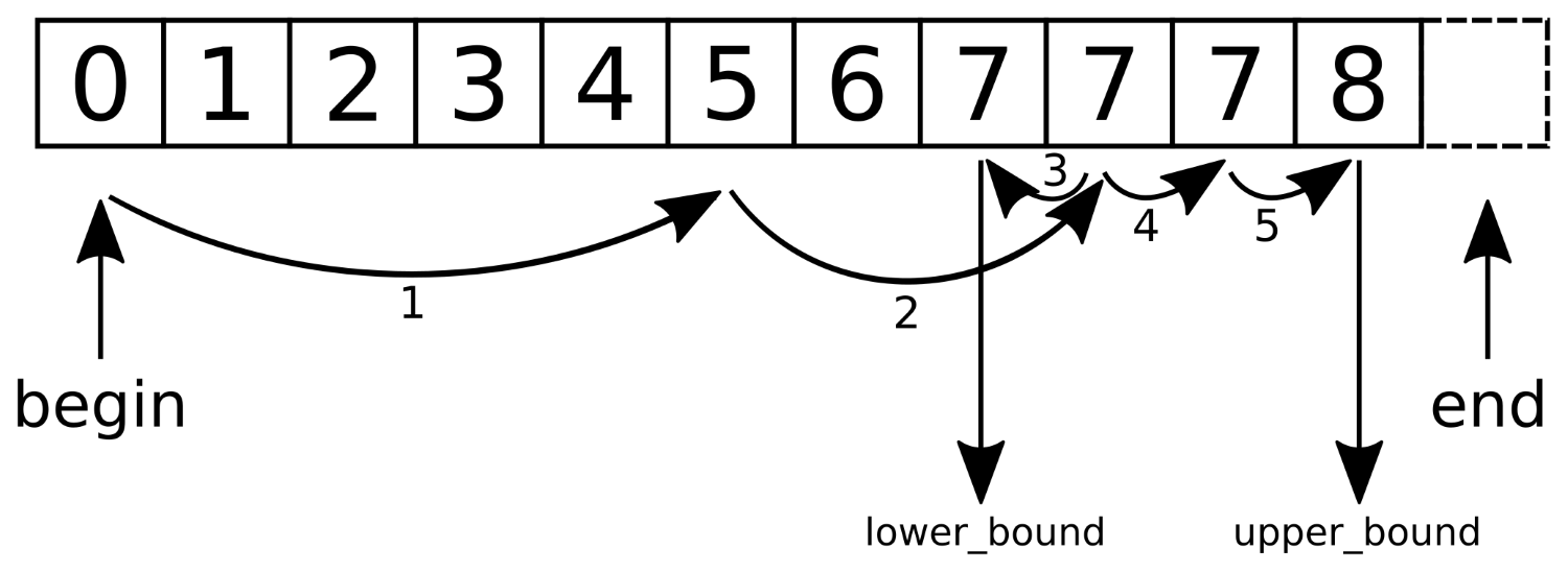
At first, equal_range uses the typical binary search approach until it trips into the range of values not smaller than the search value. Then, it splits up to a lower_bound call and an upper_bound call in order to bundle their return values in a pair as the return value.
In order to get a binary search function, which just returns the first item that fits the requirements, we could implement the following:
template <typename Iterator, typename T>
Iterator standard_binary_search(Iterator it, Iterator end_it, T value)
{
const auto potential_match (lower_bound(it, end_it, value));
if (potential_match != end_it && value == *potential_match) {
return potential_match;
}
return end_it;
}
This function uses std::lower_bound in order to find the first item not smaller than value. The resulting potential_match can then have three different cases it points to:
If our type T does not support the == operator, it must at least support the < operator for the binary search. Then, we can rewrite the comparison to !(value < *potential_match) && !(*potential_match < value). If it is neither smaller, nor larger, then it must be equal.
One potential reason why the STL does not provide such a function out of the box is the missing knowledge about the possibility that there are multiple hits, as in the diagram where we have multiple values of 7.
In a lot of applications, we get numeric data from somewhere. Before we can plot or otherwise process it, it may need to be normalized because the values differ randomly far from each other.
Usually, this would mean a little std::transform call over the data structure that holds all these values, combined with a simple scaling function. But if we do not know how large or small the values are, we need to go through the data first in order to find the right dimensions for the scaling function.
The STL contains useful functions for this purpose: std::minmax_element and std::clamp. Using these and combining them with some lambda expression glue, we can perform such a task easily.
In this section, we will normalize the values of a vector from an example numeric range to a normalized one in two different ways, one of them using std::minmax_element and one using std::clamp:
#include <iostream>
#include <vector>
#include <algorithm>
#include <iterator>
using namespace std;
static auto norm (int min, int max, int new_max)
{
const double diff (max - min);
return [=] (int val) {
return int((val - min) / diff * new_max);
};
}
static auto clampval (int min, int max)
{
return [=] (int val) -> int {
return clamp(val, min, max);
};
}
int main()
{
vector<int> v {0, 1000, 5, 250, 300, 800, 900, 321};
const auto [min_it, max_it] (
minmax_element(begin(v), end(v)));
vector<int> v_norm;
v_norm.reserve(v.size());
transform(begin(v), end(v), back_inserter(v_norm),
norm(*min_it, *max_it, 255));
copy(begin(v_norm), end(v_norm),
ostream_iterator<int>{cout, ", "});
cout << 'n';
transform(begin(v), end(v), begin(v_norm),
clampval(0, 255));
copy(begin(v_norm), end(v_norm),
ostream_iterator<int>{cout, ", "});
cout << 'n';
}
$ ./reducing_range_in_vector
0, 255, 1, 63, 76, 204, 229, 81,
0, 255, 5, 250, 255, 255, 255, 255,
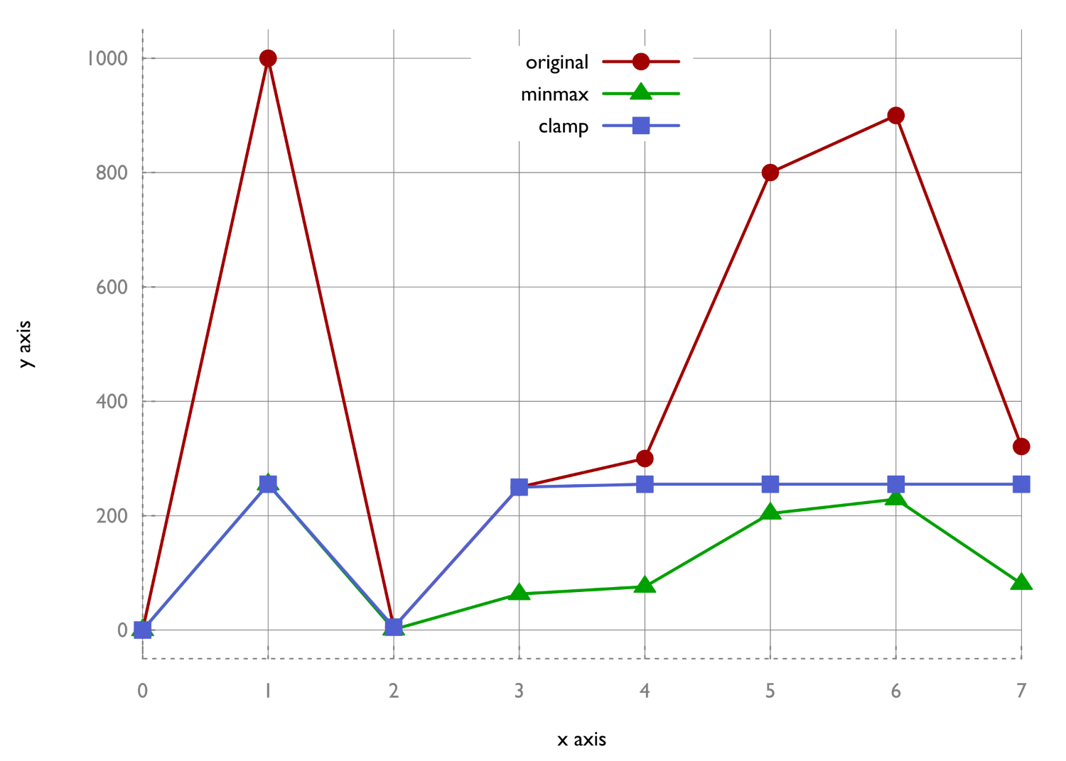
Apart from std::transform we used two algorithms:
std::minmax_element simply accepts the begin and end iterators of an input range. It loops through the range and records the largest and the smallest element on the way to its end. These values are returned in a pair, which we then used for our scaling function.
The std::clamp function, in contrast, does not operate on an iterable range. It accepts three values: an input value, a min value, and a max value. The output of this function is the input value cut-off in a way that it lies between the allowed minimum and maximum. We could also write max(min_val, min(max_val, x)) instead of std::clamp(x, min_val, max_val).
Searching for a string in a string is a slightly different problem than finding one object in a range. On the one hand, a string is, of course, an iterable range (of characters) too. On the other hand, finding a string in a string means finding a range in another range. And this comes along with multiple comparisons per potential match position, so we need some other algorithm for that.
std::string already contains a find function, which can do exactly what we are talking about; nevertheless we'll concentrate on std::search in this section. Although std::search might be used on strings mostly, it works on all kinds of containers. The more interesting feature of std::search is that since C++17, it has a slightly different additional interface and allows for simply exchanging the search algorithm itself. These algorithms are optimized and can be freely chosen by the user, depending on what is better in which use case. Additionally, we could implement our own search algorithms and plug them into std::search if we ever come up with anything better than what is already provided.
We will use the new std::search function with strings and try its different variations with searcher objects:
#include <iostream>
#include <string>
#include <algorithm>
#include <iterator>
#include <functional>
using namespace std;
template <typename Itr>
static void print(Itr it, size_t chars)
{
copy_n(it, chars, ostream_iterator<char>{cout});
cout << 'n';
}
int main()
{
const string long_string {
"Lorem ipsum dolor sit amet, consetetur"
" sadipscing elitr, sed diam nonumy eirmod"};
const string needle {"elitr"};
{
auto match (search(begin(long_string), end(long_string),
begin(needle), end(needle)));
print(match, 5);
} {
auto match (search(begin(long_string), end(long_string),
default_searcher(begin(needle), end(needle))));
print(match, 5);
} {
auto match (search(begin(long_string), end(long_string),
boyer_moore_searcher(begin(needle),
end(needle))));
print(match, 5);
} {
auto match (search(begin(long_string), end(long_string),
boyer_moore_horspool_searcher(begin(needle),
end(needle))));
print(match, 5);
}
}$ ./pattern_search_string
elitr
elitr
elitr
elitr
We utilized four different ways to use std::search in order to get exactly the same result. Which one should we prefer in what situation?
Let's assume our large string within which we search the pattern is called s, and the pattern is called p. Then, std::search(begin(s), end(s), begin(p), end(p)); and std::search(begin(s), end(s), default_searcher(begin(p), end(p)); do exactly the same thing.
The other searcher function objects are implemented with more sophisticated search algorithms:
What makes the other algorithms so special? The Boyer-Moore algorithm was developed with a specific idea--the search pattern is compared with the string, beginning at the pattern's end, from right to left. If the character in the search string differs from the character in the pattern at the overlay position and does not even occur in the pattern, then it is clear that the pattern can be shifted over the search string by its full length. Have a look at the following diagram, where this happens in step 1. If the character being currently compared differs from the pattern's character at this position but is contained by the pattern, then the algorithm knows by how many characters the pattern needs to be shifted to the right in order to correctly align to at least that character, and then, it starts over with the right-to-left comparison. In the diagram, this happens in step 2. This way, the Boyer-Moore algorithm can omit a whole lot of unnecessary comparisons, compared with a naive search implementation:
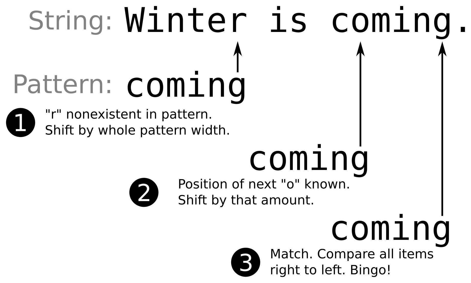
Of course, this would have become the new default search algorithm if it hadn't brought its own trade-offs. It is faster than the default algorithm, but it needs fast lookup data structures in order to determine which characters are contained in the search pattern and at which offset they are located. The compiler will select differently complex implementations of those, depending on the underlying types of which the pattern consists (varying between hash maps for complex types and primitive lookup tables for types such as char). In the end, this means that the default search implementation will be faster if the search string is not too large. If the search itself takes some significant time, then the Boyer-Moore algorithm can lead to performance gains in the dimension of a constant factor.
The Boyer-Moore-Horspool algorithm is a simplification of the Boyer-Moore algorithm. It drops the bad character rule, which leads to shifts of the whole pattern width if a search string character that does not occur in the pattern string is found. The trade-off of this decision is that it is slightly slower than the unmodified version of Boyer-Moore, but it also needs fewer data structures for its operation.
When there are very large amounts of numeric data that need to be processed in some situations, it may not be possible to process it all in feasible time. In such situations, the data could be sampled in order to reduce the total amount of data for further processing, which then speeds up the whole program. In other situations, this might be done not to reduce the amount of work for processing but for saving or transferring the data.
A naive idea of sampling could be to only pick every Nth data point. This might be fine in a lot of cases, but in signal processing, for example, it could lead to a mathematical phenomenon called aliasing. If the distance between every sample is varied by a small random offset, aliasing can be reduced. Have a look at the following diagram, which shows an extreme case just to illustrate the point--while the original signal consists of a sine wave, the triangle points on the graph are sampling points that are sampled at exactly every 100th data point. Unfortunately, the signal has the same y-value at these points! The graph which results from connecting the dots looks like a perfectly straight horizontal line. The square points, however, show what we get when we sample every 100 + random(-15, +15) points. Here, the signal still looks very different from the original signal, but it is at least not completely gone as in the fixed step size sampling case.
The std::sample function does not add random alterations to sample points with fixed offset but chooses completely random points; therefore, it works a bit differently from this example:
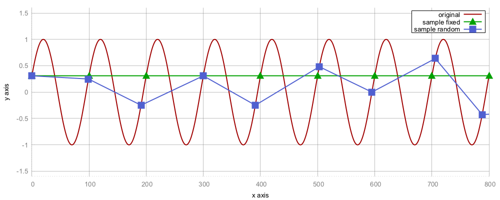
We will sample a very large vector of random data. This random data shows a normal distribution. After sampling it, the resulting points should still show a normal distribution, which we will check:
#include <iostream>
#include <vector>
#include <random>
#include <algorithm>
#include <iterator>
#include <map>
#include <iomanip>
using namespace std;
int main()
{
const size_t data_points {100000};
const size_t sample_points {100};
const int mean {10};
const size_t dev {3};random_device rd;
mt19937 gen {rd()};
normal_distribution<> d {mean, dev};
vector<int> v;
v.reserve(data_points);
generate_n(back_inserter(v), data_points,
[&] { return d(gen); });
vector<int> samples;
v.reserve(sample_points);
sample(begin(v), end(v), back_inserter(samples),
sample_points, mt19937{random_device{}()});
map<int, size_t> hist;
for (int i : samples) { ++hist[i]; }
for (const auto &[value, count] : hist) {
cout << setw(2) << value << " "
<< string(count, '*') << 'n';
}
}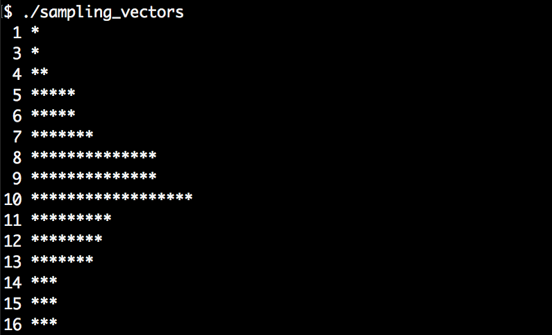
The std::sample algorithm is a new algorithm, which came with C++17. Its signature looks like this:
template<class InIterator, class OutIterator,
class Distance, class UniformRandomBitGenerator>
OutIterator sample(InIterator first, InIterator last,
SampleIterator out, Distance n,
UniformRandomBitGenerator&& g);
The input range is denoted by the first and last iterators, while out is the output operator. These iterators have exactly the same function as in std::copy; items are copied from one range to the other. The std::sample algorithm is special in the regard that it will copy only a part of the input range because it samples only n items. It uses uniform distribution internally, so every data point in the source range gets chosen with the same probability.
When testing code that must deal with sequences of inputs where the order of the arguments is not important, it is beneficial to test whether it results in the same output for all possible permutations of that input. Such a test could, for example, check whether a self-implemented sort algorithm sorts correctly.
No matter for what reason we need all permutations of some value range, std::next_permutation can conveniently do it for us. We can invoke it on a modifiable range, and it changes the order of its items to the next lexicographical permutation.
In this section, we will write a program that reads multiple word strings from a standard input, and then we will use std::next_permutation to generate and print all the permutations of those strings:
#include <iostream>
#include <vector>
#include <string>
#include <iterator>
#include <algorithm>
using namespace std;
int main()
{
vector<string> v {istream_iterator<string>{cin}, {}};
sort(begin(v), end(v));
do {
copy(begin(v), end(v),
ostream_iterator<string>{cout, ", "});
cout << 'n';
} while (next_permutation(begin(v), end(v)));
}
$ echo "a b c" | ./input_permutations
a, b, c,
a, c, b,
b, a, c,
b, c, a,
c, a, b,
c, b, a,
The std::next_permutation algorithm is a bit weird to use. This is because it accepts only a begin/end pair of iterators and then returns true if it is able to find the next permutation. Otherwise, it returns false. But what does the next permutation even mean?
The algorithm with which std::next_permutation finds the next lexicographical order of the items, works as follows:
The individually permuted orders we get out of this will always appear in the same sequence. In order to see all the possible permutations, we sorted the array first, because if we entered "c b a", for example, the algorithm would terminate immediately, as this already is the last lexicographic order of the elements.
Imagine that we have a sorted list of things, and someone else comes up with another sorted list of things, and we want to share the lists with each other. The best idea is to combine both the lists. The combination of both the lists should be sorted too, as this way, it is easy to look it up for specific items.
Such an operation is also called a merge. In order to merge two sorted ranges of items, we would intuitively create a new range and feed it with items from both the lists. For every item transfer, we would have to compare the frontmost items of our input ranges in order to always select the smallest one from what is left from the input. Otherwise, the output range would not be sorted any longer. The following diagram illustrates it better:
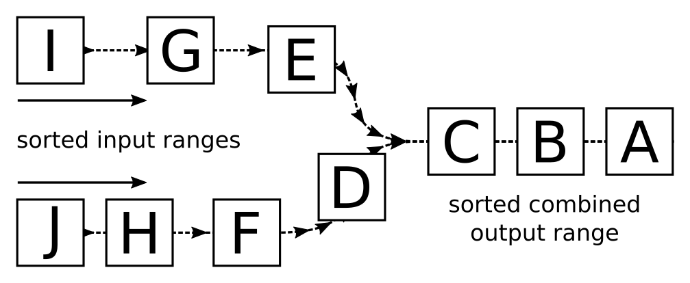
The std::merge algorithm can do exactly that for us, so we do not need to fiddle around too much. In this section, we will see how to use the algorithm.
We are going to build up a cheap dictionary of one-to-one mappings from English words to their German translations, and store them in std::deque structures. The program will read such a dictionary from a file and one from standard input, and print one large merged dictionary on the standard output again.
#include <iostream>
#include <algorithm>
#include <iterator>
#include <deque>
#include <tuple>
#include <string>
#include <fstream>
using namespace std;
using dict_entry = pair<string, string>;
namespace std {
ostream& operator<<(ostream &os, const dict_entry p)
{
return os << p.first << " " << p.second;
}
istream& operator>>(istream &is, dict_entry &p)
{
return is >> p.first >> p.second;
}
}
template <typename IS>
deque<dict_entry> from_instream(IS &&is)
{
deque<dict_entry> d {istream_iterator<dict_entry>{is}, {}};
sort(begin(d), end(d));
return d;
}
int main()
{
const auto dict1 (from_instream(ifstream{"dict.txt"}));
const auto dict2 (from_instream(cin));
merge(begin(dict1), end(dict1),
begin(dict2), end(dict2),
ostream_iterator<dict_entry>{cout, "n"});
}
car auto
cellphone handy
house haus
$ echo "table tisch fish fisch dog hund" | ./dictionary_merge
car auto
cellphone handy
dog hund
fish fisch
house haus
table tisch
The std::merge algorithm accepts two pairs of begin/end iterators, which denote the input ranges. These ranges must be sorted. The fifth parameter is an output iterator that accepts the incoming items during the merge.
There is also a variant called std::inplace_merge. This algorithm does the same as the other, but it does not need an output iterator because it works in place, as the name already suggests. It takes three parameters: a begin iterator, a middle iterator, and an end iterator. These iterators must all reference data in the same data structure. The middle iterator is at the same time the end iterator of the first range, and the begin iterator of the second range. This means that this algorithm handles a single range, which actually consists of two consecutive ranges, such as, for example, {A, C, B, D}. The first subrange is {A, C} and the second subrange is {B, D}. The std::inplace_merge algorithm can then merge both within the same data structure, which results in {A, B, C, D}.
We will cover the following recipes in this chapter:
In the last chapter, we visited basic STL algorithms and performed simple tasks with them in order to get a feeling of the typical STL interface: most STL algorithms accept one or more ranges in the form of iterator pairs as input/output parameters. They often also accept predicate functions, custom comparison functions, or transformation functions. In the end, they mostly return iterators again because these can often be fed into some other algorithm afterward.
While STL algorithms aim to be minimal, their interfaces also try to be as general as possible. This enables maximum code reuse potential but does not always look too pretty. An experienced C++ coder who knows all algorithms has a better time reading other people's code if it tries to express as many ideas using STL algorithms as possible. This leads to a maximized common ground of comprehension between coder and reader. A programmer's brain can simply parse the name of a well-known algorithm more quickly than it can understand a complex loop, which does a mainly similar, but in some detail a slightly different, job.
At this point, we are using STL data structures so intuitively that we can nicely avoid pointers, raw arrays, and other crude legacy structures. The next step is lifting our comprehension of STL algorithms up to the levels where we can avoid the use of handcrafted loop-control-structure complexes by expressing them in terms of well-known STL algorithms. Often, this is a real improvement because code becomes simply shorter and more readable while at the same time being more general and data-structure agnostic. It is practically always possible to avoid writing handcrafted loops and taking an algorithm out of the std namespace instead, but sometimes, it admittedly leads to awkward code. We are not going to differentiate between what is awkward and what is not; we'll only explore the possibilities.
In this chapter, we will use STL algorithms in creative ways in order to look for new horizons and to see how things can be implemented with modern C++. On the way, we will implement our own STL-like algorithms, which can easily be combined with existing data structures and other algorithms designed in the same way. We will also combine existing STL algorithms to get new algorithms, which were not there before. Such combined algorithms allow for more complex algorithms on top of the existing ones, while they are themselves extremely short and readable this way. While on this little trip, we will also see where exactly STL algorithms suffer from reusability or prettiness. Only when we know all the ways well can we best decide which way is the right one.
The so-called trie data structure poses an interesting way to store data in an easily searchable manner. When segmenting sentences of text into lists of words, it is often possible to combine the first few words that some sentences have in common.
Let's have a look at the following diagram, where the sentences "hi how are you" and "hi how do you do" are saved in a tree-like data structure. The first words they have in common are "hi how", and then they differ and split up like a tree:
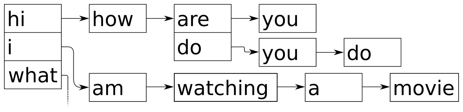
Because the trie data structure combines common prefixes, it is also called prefix tree. It is very easy to implement such a data structure with what the STL gives us already. This section concentrates on implementing our own trie class.
In this section, we will implement our own prefix tree only made from STL data structures and algorithms.
#include <iostream>
#include <optional>
#include <algorithm>
#include <functional>
#include <iterator>
#include <map>
#include <vector>
#include <string>
using namespace std;
template <typename T>
class trie
{
map<T, trie> tries;
public:
template <typename It>
void insert(It it, It end_it) {
if (it == end_it) { return; }
tries[*it].insert(next(it), end_it);
}
template <typename C>
void insert(const C &container) {
insert(begin(container), end(container));
}
void insert(const initializer_list<T> &il) {
insert(begin(il), end(il));
}
void print(vector<T> &v) const {
if (tries.empty()) {
copy(begin(v), end(v),
ostream_iterator<T>{cout, " "});
cout << 'n';
}
for (const auto &p : tries) {
v.push_back(p.first);
p.second.print(v);
v.pop_back();
}
}
void print() const {
vector<T> v;
print(v);
}
template <typename It>
optional<reference_wrapper<const trie>>
subtrie(It it, It end_it) const {
if (it == end_it) { return ref(*this); }
auto found (tries.find(*it));
if (found == end(tries)) { return {}; }
return found->second.subtrie(next(it), end_it);
}
template <typename C>
auto subtrie(const C &c) {
return subtrie(begin(c), end(c));
}
};
int main()
{
trie<string> t;
t.insert({"hi", "how", "are", "you"});
t.insert({"hi", "i", "am", "great", "thanks"});
t.insert({"what", "are", "you", "doing"});
t.insert({"i", "am", "watching", "a", "movie"});
cout << "recorded sentences:n";
t.print();
cout << "npossible suggestions after "hi":n";
if (auto st (t.subtrie(initializer_list<string>{"hi"}));
st) {
st->get().print();
}
}
$ ./trie
recorded sentences:
hi how are you
hi i am great thanks
i am watching a movie
what are you doing
possible suggestions after "hi":
how are you
i am great thanks
Interestingly, the code for word sequence insertion is shorter and simpler than the code for looking up a given word sequence in a subtrie. So, let's first have a look at the insertion code:
template <typename It>
void trie::insert(It it, It end_it) {
if (it == end_it) { return; }
tries[*it].insert(next(it), end_it);
}
The pair of iterators, it and end_it, represent the word sequence to be inserted. The tries[*it] element looks up the first word in the sequence in the subtrie, and then, .insert(next(it), end_it) restarts the same function on that lower subtrie, with the iterator one word further advanced. The if (it == end_it) { return; } line just aborts the recursion. The empty return statement does nothing, which is a bit weird at first. All the insertion happens in the tries[*it] statement. The bracket operator [] of std::map either returns an existing item for the given key or it creates one with that key. The associated value (the mapped type is a trie in this recipe) is constructed from its default constructor. This way, we are implicitly creating a new trie branch whenever we are looking up unknown words.
Looking up in a subtrie looks more complicated because we were not able to hide so much in implicit code:
template <typename It>
optional<reference_wrapper<const trie>>
subtrie(It it, It end_it) const {
if (it == end_it) { return ref(*this); }
auto found (tries.find(*it));
if (found == end(tries)) { return {}; }
return found->second.subtrie(next(it), end_it);
}
This code basically revolves around the auto found (tries.find(*it)); statement. Instead of looking up the next deeper trie node using the bracket operator ([]), we use find. If we use the [] operator for lookups, the trie will create missing items for us, which is not what we want when just looking up whether an item exists! (By the way, try doing that. The class method is const, so this will not even be possible. This can be quite a life saver, which helps us in preventing bugs.)
Another scary looking detail is the return type, optional<reference_wrapper<const trie>>. We chose std::optional as the wrapper because it is possible that there is no such subtrie for the input sequence we are looking for. If we only inserted "hello my friend", there will be no "goodbye my friend" sequence to look up. In such cases, we just return {}, which gives the caller an empty optional object. This still does not explain why we use reference_wrapper instead of just writing optional<const trie &>. The point here is that an optional instance with a member variable of the trie& type is not reassignable and hence would not compile. Implementing a reference using reference_wrapper leads to reassignable objects.
When entering something into a search engine on the Internet, the interface often tries to guess how the full search query will look. This guessing is usually based on popular search queries from the past. Sometimes, such search engine guesses are quite funny because it appears that people type weird queries into search engines.

In this section, we are going to use the trie class that we implemented in the previous recipe and build a little search query suggestion engine.
In this section, we will implement a terminal app, which accepts some input and then tries to guess what the user might want to look for, based on a cheap text file database:
#include <iostream>
#include <optional>
#include <algorithm>
#include <functional>
#include <iterator>
#include <map>
#include <list>
#include <string>
#include <sstream>
#include <fstream>
using namespace std;
template <typename T>
class trie
{
map<T, trie> tries;
public:
template <typename It>
void insert(It it, It end_it) {
if (it == end_it) { return; }
tries[*it].insert(next(it), end_it);
}
template <typename C>
void insert(const C &container) {
insert(begin(container), end(container));
}
void insert(const initializer_list<T> &il) {
insert(begin(il), end(il));
}
void print(list<T> &l) const {
if (tries.empty()) {
copy(begin(l), end(l),
ostream_iterator<T>{cout, " "});
cout << 'n';
}
for (const auto &p : tries) {
l.push_back(p.first);
p.second.print(l);
l.pop_back();
}
}
void print() const {
list<T> l;
print(l);
}
template <typename It>
optional<reference_wrapper<const trie>>
subtrie(It it, It end_it) const {
if (it == end_it) { return ref(*this); }
auto found (tries.find(*it));
if (found == end(tries)) { return {}; }
return found->second.subtrie(next(it), end_it);
}
template <typename C>
auto subtrie(const C &c) const {
return subtrie(begin(c), end(c));
}
};
static void prompt()
{
cout << "Next input please:n > ";
}
int main()
{
trie<string> t;
fstream infile {"db.txt"};
for (string line; getline(infile, line);) {
istringstream iss {line};
t.insert(istream_iterator<string>{iss}, {});
}
prompt();
for (string line; getline(cin, line);) {
istringstream iss {line};
if (auto st (t.subtrie(istream_iterator<string>{iss}, {}));
st) {
cout << "Suggestions:n";
st->get().print();
} else {
cout << "No suggestions found.n";
}
cout << "----------------n";
prompt();
}
}
do ghosts exist
do goldfish sleep
do guinea pigs bite
how wrong can you be
how could trump become president
how could this happen to me
how did bruce lee die
how did you learn c++
what would aliens look like
what would macgiver do
what would bjarne stroustrup do
...
hi how are you
hi i am great thanks
do ghosts exist
do goldfish sleep
do guinea pigs bite
how wrong can you be
how could trump become president
how could this happen to me
how did bruce lee die
how did you learn c++
what would aliens look like
what would macgiver do
what would bjarne stroustrup do
what would chuck norris do
why do cats like boxes
why does it rain
why is the sky blue
why do cats hate water
why do cats hate dogs
why is c++ so hard
$ ./word_suggestion
Next input please:
> what would
Suggestions:
aliens look like
bjarne stroustrup do
chuck norris do
macgiver do
----------------
Next input please:
> why do
Suggestions:
cats hate dogs
cats hate water
cats like boxes
----------------
Next input please:
>
How a trie works was explained in the last recipe, but how we fill it and how we query it looks a bit strange here. Let's have a closer look at the code snippet that fills the empty trie with the content of the text database file:
fstream infile {"db.txt"};
for (string line; getline(infile, line);) {
istringstream iss {line};
t.insert(istream_iterator<string>{iss}, {});
}
The loop fills the string line with the content of the text file, line by line. Then, we copy the string into an istringstream object. From such an input stream object, we can create an istream_iterator, which is useful because our trie does not only accept a container instance for looking up subtries but also primarily iterators. This way, we do not need to construct a vector or a list of words and can directly consume the string. The last piece of unnecessary memory allocations could be avoided by moving the content of line into iss. Unfortunately, std::istringstream does not provide a constructor that accepts std::string values to be moved. It will copy its input string, nevertheless.
When reading the user's input to look it up in the trie, we use exactly the same strategy but we do not use an input file stream. We use std::cin, instead. This works completely identically for our use case because trie::subtrie works with iterators just as trie::insert does.
It is possible to add counter variables to each node of the trie. This way, it is possible to count how often a prefix occurs in some input. From that, we could sort our suggestions by their occurrence frequency, which is actually what search engines do. Word suggestions for smartphone touchscreen text input could also be implemented this way.
This modification is left as an exercise for the reader.
The Fourier transformation is a very important and famous formula in signal processing. It was invented nearly 200 years ago, but with computers, the number of use cases for it really skyrocketed. It is used in audio/image/video compression, audio filters, medical imaging devices, cell phone apps that identify music tracks while listening to them on the fly, and so on.
Because of the vastness of general numeric application scenarios (not only because of the Fourier transformation of course), the STL also tries to be useful in the context of numeric computation. The Fourier transformation is only one example among them but a tricky one too. The formula itself looks like the following:
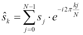
The transformation it describes is basically a sum. Each element of the sum is the multiplication of a data point of the input signal vector, and the expression exp(-2 * i * ...). The maths behind this is a bit scary for everyone who does not know about complex numbers (or who just does not like maths), but it is also not really necessary to completely understand the maths in order to implement it. When having a close look at the formula, it says that the sum symbol loops over every data point of the signal (which is N elements long) using the loop variable j. The variable k is another loop variable because the Fourier transformation is not for calculating a single value, but a vector of values. In this vector, every data point represents the intensity and phase of a certain repetitive wave frequency, which is or is not a part of the original signal. When implementing this with manual loops, we will end up with code similar to the following:
csignal fourier_transform(const csignal &s) {
csignal t(s.size());
const double pol {-2.0 * M_PI / s.size()};
for (size_t k {0}; k < s.size(); ++k) {
for (size_t j {0}; j < s.size(); ++j) {
t[k] += s[j] * polar(1.0, pol * k * j);
}
}
return t;
}
The csignal type may be an std::vector vector of complex numbers. For complex numbers, there is an std::complex STL class, which helps represent those. The std::polar function basically does the exp(-i * 2 * ...) part.
This works well already, but we are going to implement it using STL tools.
In this section, we are going to implement the Fourier transformation and its backward transformation and then play around with it to transform some signals:
#include <iostream>
#include <complex>
#include <vector>
#include <algorithm>
#include <iterator>
#include <numeric>
#include <valarray>
#include <cmath>
using namespace std;
using cmplx = complex<double>;
using csignal = vector<cmplx>;
class num_iterator {
size_t i;
public:
explicit num_iterator(size_t position) : i{position} {}
size_t operator*() const { return i; }
num_iterator& operator++() {
++i;
return *this;
}
bool operator!=(const num_iterator &other) const {
return i != other.i;
}
};
csignal fourier_transform(const csignal &s, bool back = false)
{
csignal t (s.size());
const double pol {2.0 * M_PI * (back ? -1.0 : 1.0)};
const double div {back ? 1.0 : double(s.size())};
auto sum_up ([=, &s] (size_t j) {
return [=, &s] (cmplx c, size_t k) {
return c + s[k] *
polar(1.0, pol * k * j / double(s.size()));
};
});
auto to_ft ([=, &s](size_t j){
return accumulate(num_iterator{0},
num_iterator{s.size()},
cmplx{},
sum_up(j))
/ div;
});
transform(num_iterator{0}, num_iterator{s.size()},
begin(t), to_ft);
return t;
}
static auto gen_cosine (size_t period_len){
return [period_len, n{0}] () mutable {
return cos(double(n++) * 2.0 * M_PI / period_len);
};
}
static auto gen_square_wave (size_t period_len)
{
return [period_len, n{period_len*7/4}] () mutable {
return ((n++ * 2 / period_len) % 2) * 2 - 1.0;
};
}
template <typename F>
static csignal signal_from_generator(size_t len, F gen)
{
csignal r (len);
generate(begin(r), end(r), gen);
return r;
}
static void print_signal (const csignal &s)
{
auto real_val ([](cmplx c) { return c.real(); });
transform(begin(s), end(s),
ostream_iterator<double>{cout, " "}, real_val);
cout << 'n';
}
int main()
{
const size_t sig_len {100};
auto cosine (signal_from_generator(sig_len,
gen_cosine( sig_len / 2)));
auto square_wave (signal_from_generator(sig_len,
gen_square_wave(sig_len / 2)));
auto trans_sqw (fourier_transform(square_wave));
fill (next(begin(trans_sqw), 10), prev(end(trans_sqw), 10), 0);
auto mid (fourier_transform(trans_sqw, true));
print_signal(cosine);
print_signal(fourier_transform(cosine));
print_signal(mid);
print_signal(trans_sqw);
print_signal(square_wave);
print_signal(fourier_transform(square_wave));
}
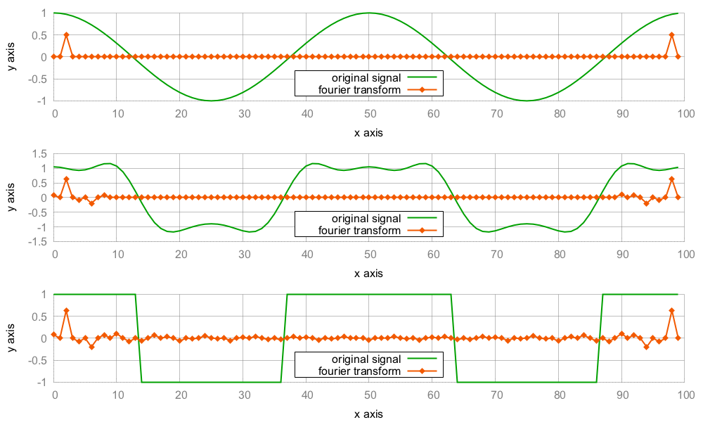
This program contains two complicated sections. One is the Fourier transformation itself, and the other is the generation of signals with mutable lambda expressions.
Let's concentrate on the Fourier transformation first. The core of the raw loop implementation (which we did not use for our implementation but had a look at in the introduction) looks like the following:
for (size_t k {0}; k < s.size(); ++k) {
for (size_t j {0}; j < s.size(); ++j) {
t[k] += s[j] * polar(1.0, pol * k * j / double(s.size()));
}
}
With the STL algorithms, std::transform and std::accumulate, we wrote code, which can be summarized to the following pseudo code:
transform(num_iterator{0}, num_iterator{s.size()}, ...
accumulate((num_iterator0}, num_iterator{s.size()}, ...
c + s[k] * polar(1.0, pol * k * j / double(s.size()));
The result is exactly the same compared with the loop variant. This is arguably an example situation where the strict use of STL algorithms does not lead to better code. Nevertheless, this algorithm implementation is agnostic over the data structure choice. It would also work on lists (although that would not make too much sense in our situation). Another upside is that the C++17 STL algorithms are easy to parallelize (which we examine in another chapter of this book), whereas raw loops have to be restructured to support multiprocessing (unless we use external libraries like OpenMP for example, but these do actually restructure the loops for us).
The other complicated part was the signal generation. Let's have another look at gen_cosine:
static auto gen_cosine (size_t period_len)
{
return [period_len, n{0}] () mutable {
return cos(double(n++) * 2.0 * M_PI / period_len);
};
}
Each instance of the lambda expression represents a function object that modifies its own state on every call. Its state consists of the variables, period_len and n. The n variable is the one which is modified on every call. The signal has a different value at every time point, and n++ represents the increasing time points. In order to get an actual signal vector out of it, we created the helper signal_from_generator:
template <typename F>
static auto signal_from_generator(size_t len, F gen)
{
csignal r (len);
generate(begin(r), end(r), gen);
return r;
}
This helper allocates a signal vector with a length of choice and calls std::generate to fill it with data points. For every item of the vector r, it calls the function object gen once, which is just the kind of self-modifying function object we can create with gen_cosine.
There are different possibilities to calculate the numerical error between a target value and an actual value. Measuring the difference between signals consisting of many data points usually involves loops and subtraction of corresponding data points, and so on.
One simple formula to calculate this error between a signal a and a signal b is the following:
For every i, it calculates a[i] - b[i], squares that difference (this way, negative and positive differences become comparable), and, finally, sums those values up. This is again a situation where one could use a loop, but for fun reasons, we will do it with an STL algorithm. The good thing is that we get data-structure independence for free this way. Our algorithm will work on vectors and on list-like data structures, where no direct indexing is possible.
In this section, we are going to create two signals and calculate their error sum:
#include <iostream>
#include <cmath>
#include <algorithm>
#include <numeric>
#include <vector>
#include <iterator>
using namespace std;
int main()
{
const size_t sig_len {100};
vector<double> as (sig_len); // a for analog
vector<int> ds (sig_len); // d for digital
auto sin_gen ([n{0}] () mutable {
return 5.0 * sin(n++ * 2.0 * M_PI / 100);
});
generate(begin(as), end(as), sin_gen);
copy(begin(as), end(as), begin(ds));
copy(begin(as), end(as),
ostream_iterator<double>{cout, " "});
cout << 'n';
copy(begin(ds), end(ds),
ostream_iterator<double>{cout, " "});
cout << 'n';
cout << inner_product(begin(as), end(as), begin(ds),
0.0, std::plus<double>{},
[](double a, double b) {
return pow(a - b, 2);
})
<< 'n';
}
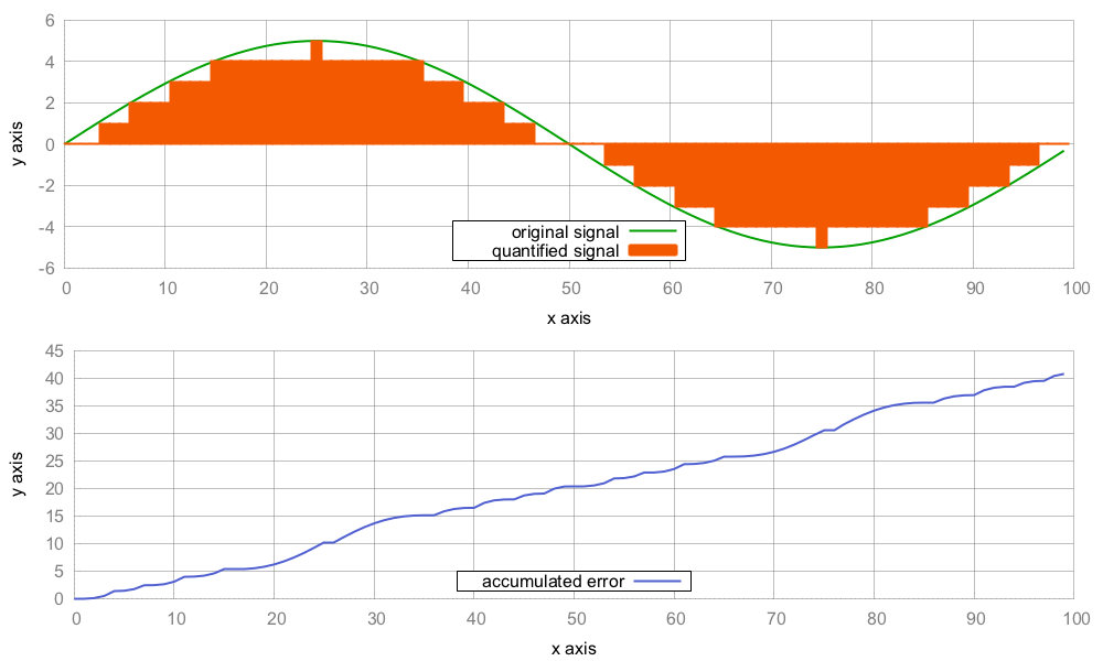
In this recipe, we stuffed the task of looping through two vectors, getting the difference between their corresponding values, squaring them, and finally summing them up into one std::inner_product call. On the way, the only code we crafted ourselves was the lambda expression [](double a, double b) { return pow(a - b, 2); }, which takes the difference of its arguments and squares it.
A glance at a possible implementation of std::inner_product shows us why and how this works:
template<class InIt1, class InIt2, class T, class F, class G>
T inner_product(InIt1 it1, InIt1 end1, InIt2 it2, T val,
F bin_op1, G bin_op2)
{
while (it1 != end1) {
val = bin_op1(val, bin_op2(*it1, *it2));
++it1;
++it2;
}
return value;
}
The algorithm accepts a pair of begin/end iterators of the first range, and another begin iterator of the second range. In our case, they are the vectors from which we want to calculate the error sum. The next character is the initial value val. We have initialized it to 0.0. Then, the algorithm accepts two binary functions, namely bin_op1 and bin_op2.
At this point, we might realize that this algorithm is really similar to std::accumulate. The only difference is that std::accumulate works on only one range. If we exchange the bin_op2(*it1, *it2) statement with *it, then we have basically restored the accumulate algorithm. We can, therefore, regard std::inner_product as a version of std::accumulate that zips a pair of input ranges.
In our case, the zipper function is pow(a - b, 2), and that's it. For the other function, bin_op1, we chose std::plus<double> because we want all the squares to be summed together.
In 1975, the mathematician Benoît Mandelbrot coined the term fractal. A fractal is a mathematical figure or set, which has certain interesting mathematical properties, but in the end, it just looks like a piece of art. Fractals also look infinitely repetitive when being zoomed in. One of the most popular fractals is the Mandelbrot set, which can be seen on the following poster:

A picture of the Mandelbrot set can be generated by iterating a specific formula:
The variables z and c are complex numbers. The Mandelbrot set consists of all such values of c for which the formula converges if it is applied often enough. This is the colored part of the poster. Some values converge earlier, some converge later, so they can be visualized with different colors. Some do not converge at all--these are painted black.
The STL comes with the useful std::complex class, and we will try to implement the formula without explicit loops, just for the sake of getting to know the STL better.
In this section, we are going to print the same image from the wall poster as a little piece of ASCII art in the terminal:
#include <iostream>
#include <algorithm>
#include <iterator>
#include <complex>
#include <numeric>
#include <vector>
using namespace std;
using cmplx = complex<double>;
static auto scaler(int min_from, int max_from,
double min_to, double max_to)
{
const int w_from {max_from - min_from};
const double w_to {max_to - min_to};
const int mid_from {(max_from - min_from) / 2 + min_from};
const double mid_to {(max_to - min_to) / 2.0 + min_to};
return [=] (int from) {
return double(from - mid_from) / w_from * w_to + mid_to;
};
}
template <typename A, typename B>
static auto scaled_cmplx(A scaler_x, B scaler_y)
{
return [=](int x, int y) {
return cmplx{scaler_x(x), scaler_y(y)};
};
}
static auto mandelbrot_iterations(cmplx c)
{
cmplx z {};
size_t iterations {0};
const size_t max_iterations {1000};
while (abs(z) < 2 && iterations < max_iterations) {
++iterations;
z = pow(z, 2) + c;
}
return iterations;
}
int main()
{
const size_t w {100};
const size_t h {40};
auto scale (scaled_cmplx(
scaler(0, w, -2.0, 1.0),
scaler(0, h, -1.0, 1.0)
));
auto i_to_xy ([=](int i) { return scale(i % w, i / w); });
auto to_iteration_count ([=](int i) {
return mandelbrot_iterations(i_to_xy(i));
});
vector<int> v (w * h);
iota(begin(v), end(v), 0);
transform(begin(v), end(v), begin(v), to_iteration_count);
auto binfunc ([w, n{0}] (auto output_it, int x) mutable {
*++output_it = (x > 50 ? '*' : ' ');
if (++n % w == 0) { ++output_it = 'n'; }
return output_it;
});
accumulate(begin(v), end(v), ostream_iterator<char>{cout},
binfunc);
}
The whole calculation took part during an std::transform call over a one-dimensional array:
vector<int> v (w * h);
iota(begin(v), end(v), 0);
transform(begin(v), end(v), begin(v), to_iteration_count);
So, what exactly happened, and why does it work this way? The to_iteration_count function is basically a call chain from i_to_xy, over scale to mandelbrot_iterations. The following diagram illustrates the transformation steps:
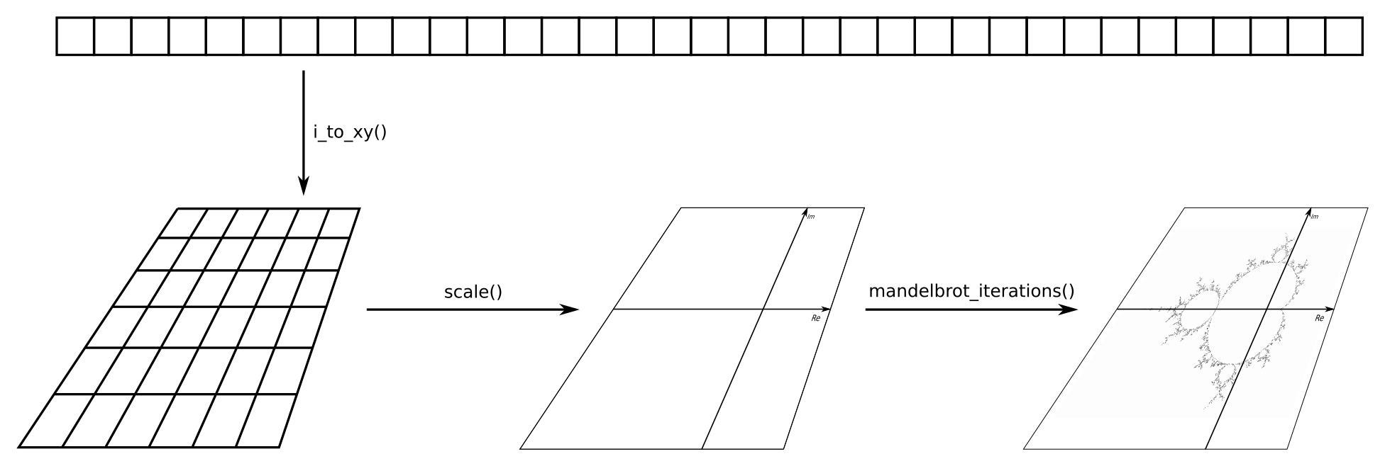
This way, we can use the index of a one-dimensional array as input, and get the number of Mandelbrot formula iterations at the point of the two-dimensional plane, which this array point represents. The good thing is that these three transformations are completely agnostic about each other. Code with such a separation of concerns can be tested very nicely because each component can be tested individually without the others. This way, it is easy to find and fix bugs, or just reason about its correctness.
In some situations, the existing STL algorithms are not enough. But nothing hinders us from implementing our own. Before solving a specific problem, we should think about it firmly in order to realize that many problems can be solved in generic ways. If we regularly pile up some new library code while solving our own problems, then we are also helping our fellow programmers when they have similar problems to solve. Key is to know when it is generic enough and when not to go for more genericity than needed--else we end up with a new general purpose language.
In this recipe, we are implementing an algorithm, which we will call split. It can split any range of items at each occurrence of a specific value, and it copies the chunks that result from that into an output range.
In this section, we are going to implement our own STL-like algorithm called split, and then we check it out by splitting an example string:
#include <iostream>
#include <string>
#include <algorithm>
#include <iterator>
#include <list>
using namespace std;
template <typename InIt, typename OutIt, typename T, typename F>
InIt split(InIt it, InIt end_it, OutIt out_it, T split_val,
F bin_func)
{
while (it != end_it) {
auto slice_end (find(it, end_it, split_val));
*out_it++ = bin_func(it, slice_end);
if (slice_end == end_it) { return end_it; }
it = next(slice_end);
}
return it;
}
int main()
{
const string s {"a-b-c-d-e-f-g"};
auto binfunc ([](auto it_a, auto it_b) {
return string(it_a, it_b);
});
list<string> l;
split(begin(s), end(s), back_inserter(l), '-', binfunc);
copy(begin(l), end(l), ostream_iterator<string>{cout, "n"});
}
$ ./split
a
b
c
d
e
f
g
The split algorithm works in a similar manner to std::transform because it accepts a pair of begin/end iterators of an input range and an output iterator. It does something with the input range, which, in the end, results in assignments to the output iterator. Apart from that, it accepts an item value called split_val and a binary function. Let's revisit the whole implementation to fully understand it:
template <typename InIt, typename OutIt, typename T, typename F>
InIt split(InIt it, InIt end_it, OutIt out_it, T split_val, F bin_func)
{
while (it != end_it) {
auto slice_end (find(it, end_it, split_val));
*out_it++ = bin_func(it, slice_end);
if (slice_end == end_it) { return end_it; }
it = next(slice_end);
}
return it;
}
The loop demands to iterate until the end of the input range. During each iteration, an std::find call is used to find the next element in the input range, which equals to split_val. In our case, that element is the dash character ('-') because we want to split our input string at all the dash positions. The next dash position is now saved in slice_end. After the loop iteration, the it iterator is put on the next item past that split position. This way, the loop jumps directly from dash to dash, instead of over every individual item.
In this constellation, the iterator it points to the beginning of the last slice, while slice_end points to the end of the last slice. Both these iterators, in combination, mark the beginning and end of the subrange that represents exactly one slice between two dash symbols. In a string, "foo-bar-baz", this would mean that we have three loop iterations and we get a pair of iterators every time, which surround one word. But we do not actually want iterators but substrings. The binary function, bin_func, does just that for us. When we called split, we gave it the following binary function:
[](auto it_a, auto it_b) {
return string(it_a, it_b);
}
The split function throws every pair of iterators through bin_func, before feeding it into the output iterator. And we actually get string instances out of bin_func, which results in "foo", "bar", and "baz":
An interesting alternative to implementing our own algorithm for splitting strings would be implementing an iterator that does the same. We are not going to implement such an iterator at this point, but let's have a brief look at such a scenario.
The iterator would need to jump between delimiters on every increment. Whenever it is dereferenced, it needs to create a string object from the iterator positions it currently points to, which it could do using a binary function such as binfunc, which we used before.
If we had an iterator class called split_iterator, instead of an algorithm split, the user code would look as follows:
string s {"a-b-c-d-e-f-g"};
list<string> l;
auto binfunc ([](auto it_a, auto it_b) {
return string(it_a, it_b);
});
copy(split_iterator{begin(s), end(s), ‘-‘, binfunc},{}, back_inserter(l));
The downside of this approach is that implementing an iterator is usually more complicated than a single function. Also, there are many subtle edges in iterator code that can lead to bugs, so an iterator solution needs more tedious testing. On the other hand, it is very simple to combine such an iterator with the other STL algorithms.
A very nice example for the composability of STL algorithms is gather. Sean Parent, principal scientist at Adobe Systems at the time, popularized this algorithm because it is both useful and short. The way it is implemented, it is the ideal poster child for the idea of STL algorithm composition.
The gather algorithm operates on ranges of arbitrary item types. It modifies the order of the items in such a way that specific items are gathered around a specific position, chosen by the caller.
In this section, we will implement the gather algorithm and a bonus variation of it. Afterward, we see how it can be put to use:
#include <iostream>
#include <algorithm>
#include <string>
#include <functional>
using namespace std;
template <typename It, typename F>
pair<It, It> gather(It first, It last, It gather_pos, F predicate)
{
return {stable_partition(first, gather_pos, not_fn(predicate)),
stable_partition(gather_pos, last, predicate)};
}
template <typename It>
void gather_sort(It first, It last, It gather_pos)
{
using T = typename std::iterator_traits<It>::value_type;
stable_sort(first, gather_pos, greater<T>{});
stable_sort(gather_pos, last, less<T>{});
}
int main()
{
auto is_a ([](char c) { return c == 'a'; });
string a {"a_a_a_a_a_a_a_a_a_a_a"};
auto middle (begin(a) + a.size() / 2);
gather(begin(a), end(a), middle, is_a);
cout << a << 'n';
gather(begin(a), end(a), begin(a), is_a);
cout << a << 'n';
gather(begin(a), end(a), end(a), is_a);
cout << a << 'n';
// This will NOT work as naively expected
gather(begin(a), end(a), middle, is_a);
cout << a << 'n';
string b {"_9_2_4_7_3_8_1_6_5_0_"};
gather_sort(begin(b), end(b), begin(b) + b.size() / 2,
less<char>{});
cout << b << 'n';
}
$ ./gather
_____aaaaaaaaaaa_____
aaaaaaaaaaa__________
__________aaaaaaaaaaa
__________aaaaaaaaaaa
_____9743201568______
Initially, the gather algorithm is hard to grasp because it is very short but has a seemingly complex task. Therefore, let's step through it:
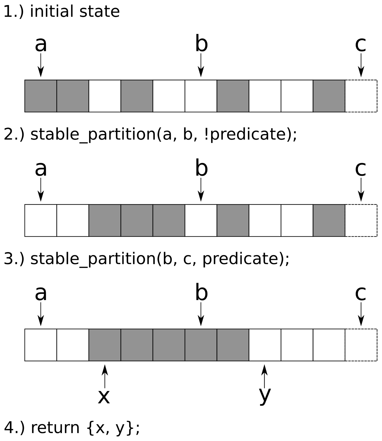
We called gather multiple times on the same range. At first, we gathered all the items around the middle of the range. Then we gathered the items around begin() and then around end() of the range. These cases are interesting because they always lead one of the std::stable_partition calls to operate on an empty range, which results in no action.
We did the last call to gather again with the parameters (begin, end, middle) of the range, and that did not work. Why? At first, this looks like a bug, but actually, it is not.
Imagine the character range, "aabb", together with a predicate function, is_character_a, which is only true for the 'a' items--if we call it with a third iterator pointing to the middle of the character range, we would observe the same bug. The reason is that the first stable_partition call would operate on the subrange, "aa", and the other stable_partition call operates on the range, "bb". This series of calls cannot result in "baab", which we initially naively hoped.
The gather_sort modification is basically the same as gather. The only difference is that it does not accept a unary predicate function but a binary comparison function, just like std::sort. And instead of calling std::stable_partition twice, it calls std::stable_sort twice.
The negation of the comparison function cannot be done with not_fn, just like we did in the gather algorithm because not_fn does not work on binary functions.
Because strings are often read from user input, they may contain wild formatting and often need to be sanitized. One example of this is strings containing too many whitespace.
In this section, we will implement a slick whitespace filtering algorithm, which removes excess whitespace from strings but leaves single whitespace characters untouched. We call that algorithm remove_multi_whitespace, and its interface will look very STL-like.
In this section, we will implement the remove_multi_whitespace algorithm and check out how it works:
#include <iostream>
#include <string>
#include <algorithm>
using namespace std;
template <typename It>
It remove_multi_whitespace(It it, It end_it)
{
return unique(it, end_it, [](const auto &a, const auto &b) {
return isspace(a) && isspace(b);
});
}
int main()
{
string s {"fooo bar t baz"};
cout << s << 'n';
s.erase(remove_multi_whitespace(begin(s), end(s)), end(s));
cout << s << 'n';
}
$ ./remove_consecutive_whitespace
fooo bar baz
fooo bar baz
We solved the whole complexity of the problem without any loop or manual comparison of items. We only provided a predicate function, which tells if two given characters are whitespace characters. Then we fed that predicate into std::unique and poof, all the excess whitespace vanished. While this chapter also contains some recipes where we had to fight a bit more to express our programs with STL algorithms, this algorithm is a really nice and short example.
How does this interesting combination work in detail? Let's have a look at a possible implementation of std::unique first:
template<typename It, typename P>
It unique(It it, It end, P p)
{
if (it == end) { return end; }
It result {it};
while (++it != end) {
if (!p(*result, *it) && ++result != it) {
*result = std::move(*it);
}
}
return ++result;
}
The loop steps over the range items, while they do not satisfy the predicate condition. At the point where an item satisfies the predicate, it moves such an item one item past the old position, where the predicate fired the last time. The version of std::unique that does not accept an additional predicate function checks whether two neighbor items are equal. This way, it wipes out repeated characters as it can , for example, transform "abbbbbbc" to "abc".
What we want is not wiping out all characters which are repetitive, but repetitive whitespace. Therefore, our predicate does not say "both argument characters are equal", but "both argument characters are whitespace characters".
One last thing to note is that neither std::unique nor remove_multi_whitespace really removes character items from the underlying string. They only move characters within the string according to their semantics and tell where its new end is. The removal of all now-obsolete characters from the new end till the old end must still be done. This is why we wrote the following:
s.erase(remove_multi_whitespace(begin(s), end(s)), end(s));
This adheres to the erase-remove idiom, which we already know from vectors and lists.
This section deals with a relatively popular task in coding interviews. The basic idea is a function, which takes a string like "aaaaabbbbbbbccc" and transforms it to a shorter string "a5b7c3". It is "a5" because there are five 'a' characters. And then it is "b7" because there are seven 'b' characters. This is a very simple compression algorithm. For normal text, it is of reduced utility because normal language is usually not so repetitive that its text representation would become shorter with this compression scheme. However, it is relatively easy to implement even if we have to do it on a whiteboard without a computer. The tricky part is that it is easy to write a buggy code if the program is not structured very well from the beginning. Dealing with strings is generally not a hard thing, but the chances of implementing buffer overflow bugs lurk around a lot here if legacy C-style formatting functions are used.
Let's try an STL approach to implementing string compression and decompression using this simple scheme.
In this section, we will implement simple compress and decompress functions for strings:
#include <iostream>
#include <string>
#include <algorithm>
#include <sstream>
#include <tuple>
using namespace std;
template <typename It>
tuple<It, char, size_t> occurrences(It it, It end_it)
{
if (it == end_it) { return {it, '?', 0}; }
const char c {*it};
const auto diff (find_if(it, end_it,
[c](char x) { return c != x; }));
return {diff, c, distance(it, diff)};
}
string compress(const string &s)
{
const auto end_it (end(s));
stringstream r;
for (auto it (begin(s)); it != end_it;) {
const auto [next_diff, c, n] (occurrences(it, end_it));
r << c << n;
it = next_diff;
}
return r.str();
}
string decompress(const string &s)
{
stringstream ss{s};
stringstream r;
char c;
size_t n;
while (ss >> c >> n) { r << string(n, c); }
return r.str();
}
int main()
{
string s {"aaaaaaaaabbbbbbbbbccccccccccc"};
cout << compress(s) << 'n';
cout << decompress(compress(s)) << 'n';
}
$ ./compress
a9b9c11
aaaaaaaaabbbbbbbbbccccccccccc
This program basically revolves around two functions: compress and decompress.
The decompress function is really simple because it only consists of variable declarations, a line of code, which actually does something, and the following return statement. The code line which does something is the following one:
while (ss >> c >> n) { r << string(n, c); }
It continuously reads the character, c, and the counter variable, n, out of the string stream, ss. The stringstream class hides a lot of string parsing magic from us at this point. While that succeeds, it constructs a decompressed string chunk into the string stream, from which the final result string can be returned back to the caller of decompress. If c = 'a' and n = 5, the expression string(n, c) will result in a string with the content, "aaaaa".
The compress function is more complex. We also wrote a little helper function for it. We called that helper function occurences. So, let's first have a glance at occurrences. The following diagram shows how it works:
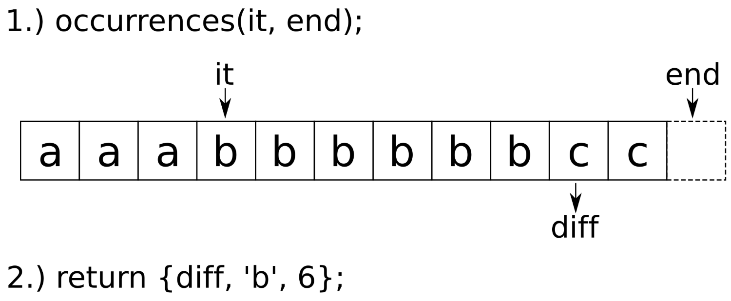
The occurences function accepts two parameters: an iterator pointing to the beginning of a character sequence within a range and the end iterator of that range. Using find_if, it finds the first character that is different from the character initially being pointed at. In the diagram, this is the iterator, diff. The difference between that new position and the old iterator position is the number of equal items (diff - it equals 6 in the diagram). After calculating this information, the diff iterator can be reused in order to execute the next search. Therefore, we pack diff, the character of the subrange, and the length of the subrange into a tuple and return it.
With the information lined up like this, we can jump from subrange to subrange and push the intermediate results into the compressed target string:
for (auto it (begin(s)); it != end_it;) {
const auto [next_diff, c, n] (occurrences(it, end_it));
r << c << n;
it = next_diff;
}
In step 4, we mentioned that the decompress function is not safe. Indeed, it can easily be exploited.
Imagine the following input string: "a00000". Compressing it will result in the substring "a1" because there is only one character, 'a'. That is followed by five times '0', which will result in "05". Together, this results in the compressed string "a105". Unfortunately, this compressed string says "105 times the character 'a'". This has nothing to do with our initial input string. Even worse, if we decompress it, we get from a six-character string to a 105-character string. Imagine the same with larger numbers--the user can easily blow up our heap usage because our algorithm is not prepared for such inputs.
In order to prevent this, the compress function could, for example, reject input with numbers, or it could mask them in a special way. And the decompress algorithm could take another conditional, which puts an upper bound on the resulting string size. I am leaving this as an exercise for you.
We will cover the following recipes in this chapter:
This chapter is devoted to string handling, parsing, and printing of arbitrary data. For such jobs, STL provides its I/O stream library. The library basically consists of the following classes, which are each depicted in gray boxes:
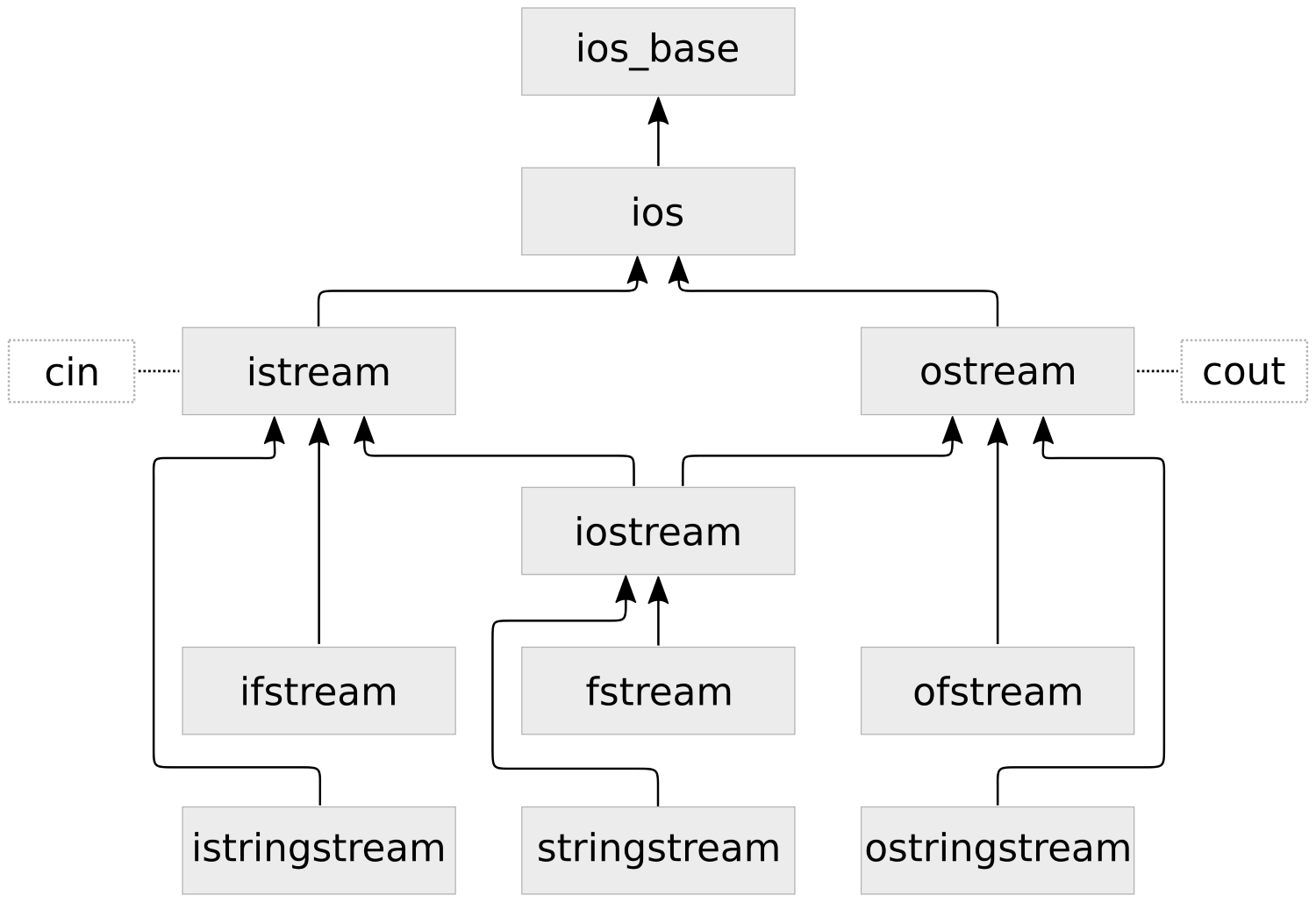
The arrows show the inheritance scheme of the classes. This might look very overwhelming at first, but we will get to use most of these classes in this chapter and get familiar with them class by class. When looking at those classes in the C++ STL documentation, we will not find them directly with these exact names. That is because the names in the diagram are what we see as application programmers, but they are really mostly just typedefs of classes with a basic_ class name prefix (for example, we will have an easier job searching the STL documentation for basic_istream rather than istream). The basic_* I/O stream classes are templates that can be specialized for different character types. The classes in the diagram are specialized on char values. We will use these specializations throughout the book. If we prefix those class names with the w character, we get wistream, wostream, and so on--these are the specialization typedefs for wchar_t instead of char, for example.
At the top of the diagram, we see std::ios_base. We will basically never use it directly, but it is listed for completeness because all other classes inherit from it. The next specialization is std::ios which embodies the idea of an object which maintains a stream of data, that can be in good state, run empty of data state (EOF), or some kind of fail state.
The first specializations we are going to actually use are std::istream and std::ostream. The "i" and the "o" prefix stand for input and output. We have seen them in our earliest days of C++ programming in the simplest examples in form of the objects std::cout and std::cin (but also std::cerr). These are instances of those classes, which are always globally available. We do data output via ostream and input via istream.
A class which inherits from both istream and ostream is iostream. It combines both input and output capabilities. When we understand how all classes from the trio consisting of istream, ostream and iostream can be used, we basically are ready to immediately put all following ones to use, too:
ifstream, ofstream and fstream inherit from istream, ostream and iostream respectively, but lift their capabilities to redirect the I/O from and to files from the computer's filesystem.
The istringstream, ostringstream and iostringstream work pretty analogously. They help build strings in memory, and/or consuming data from them.
Even C++ programmers from the very old days will know about std::string. While string handling is tedious and painful in C, especially when parsing, concatenating, copying them, and so on, std::string is a real step forward regarding simplicity and safety.
Thanks to C++11, we don't even need to copy strings when we want to transfer ownership to some other function or data structure anymore because we can move them. This way, there's not much overhead involved in most cases.
The std::string got a few new features here and there over the last few standard increments. What is completely new in C++17 is std::string_view. We will play with both a bit (but there is another recipe, which concentrates more on std::string_view-only features) to get a feeling of them and how they work in the C++17 era.
We will create strings and string views and do basic concatenation and transformation with them in this section:
#include <iostream>
#include <string>
#include <string_view>
#include <sstream>
#include <algorithm>
using namespace std;
int main()
{
string a { "a" };
auto b ( "b"s );
string_view c { "c" };
auto d ( "d"sv );
cout << a << ", " << b << 'n';
cout << c << ", " << d << 'n';
cout << a + b << 'n';
cout << a + string{c} << 'n';
ostringstream o;
o << a << " " << b << " " << c << " " << d;
auto concatenated (o.str());
cout << concatenated << 'n';
transform(begin(concatenated), end(concatenated),
begin(concatenated), ::toupper);
cout << concatenated << 'n';
}
$ ./creating_strings
a, b
c, d
ab
ac
a b c d
A B C D
Obviously, strings can be added with the + operator like numbers, but that has nothing to do with math but results in concatenated strings. In order to mix this with string_view, we need to convert to std::string first.
However, it is really important to note that when mixing strings and string views in code, we must never assume that the underlying string behind a string_view is zero terminated! This is why we would rather write "abc"s + string{some_string_view} than "abc"s + some_string_view.data(). Aside from that, std::string provides a member function, append, which can handle string_view instances, but it alters the string instead of returning a new one with the string view content appended.
If we want to do complex string concatenation with formatting and so on, we should however not do that piece by piece on string instances. The std::stringstream, std::ostringstream, and std::istringstream classes are much better suited for this, as they enhance the memory management while appending, and provide all the formatting features we know from streams in general. The std::ostringstream class is what we chose in this section because we were going to create a string instead of parsing it. An std::istringstream instance could have been instantiated from an existing string, which we could have then comfortably parsed into variables of other types. If we want to combine both, std::stringstream is the perfect all-rounder.
Especially when obtaining strings from user input, they are often polluted with unneeded white space. In another recipe, we removed excess whitespace that occurred between words.
Let's now have a look at strings that are surrounded by whitespace and remove that. The std::string has some nice helper functions for getting this job done.
In this section, we will write a helper function that identifies surrounding white space in a string and returns a copy without that, and then we are going to test it briefly.
#include <iostream>
#include <string>
#include <algorithm>
#include <cctype>
using namespace std;
string trim_whitespace_surrounding(const string &s)
{
const char whitespace[] {" tn"};
const size_t first (s.find_first_not_of(whitespace));
if (string::npos == first) { return {}; }
const size_t last (s.find_last_not_of(whitespace));
return s.substr(first, (last - first + 1));
}
int main()
{
string s {" tn string surrounded by ugly"
" whitespace tn "};
cout << "{" << s << "}n";
cout << "{"
<< trim_whitespace_surrounding(s)
<< "}n";
}
$ ./trim_whitespace
{
string surrounded by ugly whitespace
}
{string surrounded by ugly whitespace}
In this section, we used string::find_first_not_of and string::find_last_not_of. Both functions accept a C-style string, which acts as a list of characters that should be skipped while searching a different character. If we have a string instance that carries the string, "foo bar", and we call find_first_not_of("bfo ") on it, it will return us the value 5, because the 'a' character is the first one that is not in the "bfo " string. The order of the characters in the argument string is not important.
The same functions exist with inverted logic, although we did not use them in this recipe: string::find_first_of and string::find_last_of.
Similar to iterator based functions, we need to check if these functions return an actual position in the string or a value that denotes that they did not find a character position fulfilling the constraints. If they did not find one, they return string::npos.
From the character positions we retrieved from these functions in our helper function, we built us a substring without surrounding whitespace, using string::substring. This function accepts a relative offset and a string length and then returns a new string instance with its own memory, which contains only that substring. For example, string{"abcdef"}.substr(2, 2) will return us a new string "cd".
The std::string class is a really useful class because it simplifies dealing with strings so much. A flaw is that if we want to pass around a substring of it, we need to pass a pointer and a length variable, two iterators, or a copy of the substring. We did that in the previous recipe, where we removed the surrounding whitespace from a string by taking a copy of the substring range that does not contain the surrounding whitespace.
If we want to pass a string or a substring to a library that does not even support std::string, we can only provide a raw string pointer, which is a bit disappointing, because it sets us back to the old C days. Just as with the substring problem, a raw pointer does not carry information about the string length with it. This way, one would have to implement a bundle of a pointer and a string length.
In a simplified way, this is exactly what std::string_view is. It is available since C++17 and provides a way to pair a pointer to some string together with that string's size. It embodies the idea of having a reference type for arrays of data.
If we design functions which formerly accepted std::string instances as parameters, but did not change them in a way that would require the string instances to reallocate the memory that holds the actual string payload, we could now use std::string_view and be more compatible with libraries that are STL-agnostic. We could let other libraries provide a string_view view on the payload strings behind their complex string implementations and then use that in our STL code. This way, the string_view class acts as a minimal and useful interface, which can be shared among different libraries.
Another cool thing is that string_view can be used as a non-copy reference to substrings of larger string objects. There are a lot of possibilities to use it profitably. In this section, we will play around with string_view in order to get a feeling for its ups and downs. We will also see how we can hide the surrounding whitespace from strings by adapting string views instead of modifying or copying the actual string. This method avoids unnecessary copying or data modification.
We are going to implement a function that relies on some string_view features, and then, we see how many different types we can feed into it:
#include <iostream>
#include <string_view>
using namespace std;
void print(string_view v)
{
const auto words_begin (v.find_first_not_of(" tn"));
v.remove_prefix(min(words_begin, v.size()));
const auto words_end (v.find_last_not_of(" tn"));
if (words_end != string_view::npos) {
v.remove_suffix(v.size() - words_end - 1);
}
cout << "length: " << v.length()
<< " [" << v << "]n";
}
int main(int argc, char *argv[])
{
print(argv[0]);
print({});
print("a const char * array");
print("an std::string_view literal"sv);
print("an std::string instance"s);
print(" tn foobar n t ");
char cstr[] {'a', 'b', 'c'};
print(string_view(cstr, sizeof(cstr)));
}
$ ./string_view
length: 17 [./string_view]
length: 0 []
length: 20 [a const char * array]
length: 27 [an std::string_view literal]
length: 23 [an std::string instance]
length: 6 [foobar]
length: 3 [abc]
We have just seen that we can call a function that accepts a string_view argument with basically anything that is string like in the sense that it stores characters in a contiguous way. No copy of the underlying string was made in any of our print calls.
It is interesting to note that in our print(argv[0]) call, the string view automatically determined the string length because this is a zero-terminated string by convention. The other way around, one cannot assume that it is possible to determine a string_view instances's data length by counting the number of items until a zero terminator is reached. Because of this, we must always be careful about where we reach around a pointer to the string view data using string_view::data(). Usual string functions mostly assume zero termination and, thus, can buffer overflow very badly with raw pointers to the payload of a string view. It is always better to use interfaces that already expect a string view.
Apart from that, we get a lot of the luxury interface we know from std::string already.
A lot of recipes in this book read values from an input source, such as standard input or a file, and do something with it. This time we concentrate only on the reading and learn more about error handling, which becomes important if reading something from a stream did not go well and we need to handle it other than terminating the whole program.
We will only read from user input in this recipe, but as soon as we know how to do that, we also know how to read from any other stream. User input is read via std::cin, and that is essentially an input stream object, such as instances of ifstream and istringstream are.
In this section, we are going to read user input into different variables, and see how to handle errors, as well as how to do a little bit more complex tokenizing of input into useful chunks:
#include <iostream>
using namespace std;
int main()
{
cout << "Please Enter two numbers:n> ";
int x;
double y;
if (cin >> x >> y) {
cout << "You entered: " << x
<< " and " << y << 'n';
} else {
cout << "Oh no, that did not go well!n";
cin.clear();
cin.ignore(
std::numeric_limits<std::streamsize>::max(),
'n');
}
cout << "now please enter some "
"comma-separated names:n> ";
for (string s; getline(cin >> ws, s, ',');) {
if (s.empty()) { break; }
cout << "name: "" << s << ""n";
}
}
$ ./strings_from_user_input
Please Enter two numbers:
> 1 2
You entered: 1 and 2
now please enter some comma-separated names:
> john doe, ellen ripley, alice, chuck norris,,
name: "john doe"
name: "ellen ripley"
name: "alice"
name: "chuck norris"
$ ./strings_from_user_input
Please Enter two numbers:
> a b
Oh no, that did not go well!
now please enter some comma-separated names:
> bud spencer, terence hill,,
name: "bud spencer"
name: "terence hill"
We did some complex input retrieval in this section. The first noticeable thing is that we always did the retrieval and error checking at the same time.
The result of the expression cin >> x is again a reference to cin. This way, we can write cin >> x >> y >> z >> .... At the same time, it is possible to convert it into a Boolean value by using it in a Boolean context such as if conditions. The Boolean value tells us if the last read was successful. That is why we were able to write if (cin >> x >> y) {...}.
If we, for example, try to read an integer, but the input contains "foobar" as the next token, then parsing this into the integer is not possible and the stream object enters a fail state. This is only critical for the parsing attempt but not for the whole program. It is okay to reset it and then to try anything else. In our recipe program, we tried to read a list of names after a potentially failing attempt to read two numbers. In the case of a failing attempt to read those numbers in, we used cin.clear() to put cin back into a working state. But then, its internal cursor was still on what we typed instead of numbers. In order to drop this old input and clear the pipe for the names input, we used the very long expression, cin.ignore(std::numeric_limits<std::streamsize>::max(), 'n');. This is necessary to clear whatever is in the buffer at this point, because we want to start with a really fresh buffer when we ask the user for a list of names.
The following loop might look strange at first, too:
for (string s; getline(cin >> ws, s, ',');) { ... }
In the conditional part of the for loop, we use getline. The getline function accepts an input stream object, a string reference as an output parameter, and a delimiter character. By default, the delimiter character is the newline symbol. Here, we defined it to be the comma (,) character, so all the names in a list, such as "john, carl, frank", are read individually.
So far, so good. But what does it mean to provide the cin >> ws function as a stream object? This makes cin first flush all the whitespace, which lead before the next non-whitespace character and after the last comma. Looking back at the "john, carl, frank" example, we would get the substrings "john", " carl", and " frank" without using ws. Notice the unnecessary leading space characters for carl and frank? These effectively vanish because of our ws pretreatment of the input stream.
Let's say we read a text file and we want to count the number of words in the text. We define that one word is a range of characters between whitespace characters. How do we do it?
We could count the number of spaces, for example, because there must be spaces between words. In the sentence, "John has a funny little dog.", we have five space characters, so we could say there are six words.
What if we have a sentence with whitespace noise, such as " John has t anfunny little dog ."? There are way too many unnecessary spaces in this string, and it's not even only spaces. From the other recipes in this book, we already learned how we can remove such excess whitespace. So, we could first preprocess the string into a normal sentence form and then apply the strategy of counting space characters. Yes, that is doable, but there is a much easier way. Why shouldn't we use what the STL already provides us?
In addition to finding an elegant solution for this problem, we will let the user choose if we shall count the words from the standard input or a text file.
In this section, we will write a one-liner function that counts the words from an input buffer, and let the user choose where the input buffer reads from:
#include <iostream>
#include <fstream>
#include <string>
#include <algorithm>
#include <iterator>
using namespace std;
template <typename T>
size_t wordcount(T &is)
{
return distance(istream_iterator<string>{is}, {});
}
int main(int argc, char **argv)
{
size_t wc;
if (argc == 2) {
ifstream ifs {argv[1]};
wc = wordcount(ifs);
} else {
wc = wordcount(cin);
}
cout << "There are " << wc << " wordsn";
};
$ echo "foo bar baz" | ./count_all_words
There are 3 words
$ ./count_all_words count_all_words.cpp
There are 61 words
There is not much left to say; most of it has been explained while implementing it as this program is very short. One thing we could elaborate on a bit is the fact that we used std::cin and an std::ifstream instance in a completely interchangeable way. The cin is of the std::istream type, and std::ifstream inherits from std::istream. Have a look at the class inheritance diagram at the beginning of this chapter. This way, they are completely interchangeable, even at runtime.
In many cases, just printing out strings and numbers is not enough. Sometimes, numbers need to be printed as decimal numbers, sometimes as hexadecimal, and sometimes even as octal. Sometimes we want to see a "0x" prefix in front of hexadecimal numbers, sometimes not.
When printing floating-point numbers, there are also a lot of things we may want to have an influence on. Should the decimal values always be printed with the same precision? Should they be printed at all? Or perhaps, we want a scientific notation?
Apart from scientific presentation and hexadecimal, octal, and so on, we also want to present the user output in a tidy form. Some output can be arranged in tables, for example, in order to make it as readable as possible.
All these things are, of course, possible with output streams. Some of these settings are also important when parsing values from input streams. In this recipe, we will get a feeling of such so-called I/O manipulators by playing around with them. Sometimes, they appear tricky, so we will also get into some details.
In this section, we will print numbers with wildly varying format settings, in order to get familiar with I/O manipulators:
#include <iostream>
#include <iomanip>
#include <locale>
using namespace std;
void print_aligned_demo(int val,
size_t width,
char fill_char = ' ')
{
cout << "================n";
cout << setfill(fill_char);
cout << left << setw(width) << val << 'n';
cout << right << setw(width) << val << 'n';
cout << internal << setw(width) << val << 'n';
}
int main()
{
print_aligned_demo(123456, 15);
print_aligned_demo(123456, 15, '_');
cout << hex << showbase;
print_aligned_demo(0x123abc, 15);
cout << oct;
print_aligned_demo(0123456, 15);
cout << "A hex number with upper case letters: "
<< hex << uppercase << 0x123abc << 'n';
cout << "A number: " << 100 << 'n';
cout << dec;
cout << "Oops. now in decimal again: " << 100 << 'n';
cout << "true/false values: "
<< true << ", " << false << 'n';
cout << boolalpha
<< "true/false values: "
<< true << ", " << false << 'n';
cout << "doubles: "
<< 12.3 << ", "
<< 12.0 << ", "
<< showpoint << 12.0 << 'n';
cout << "scientific double: " << scientific
<< 123000000000.123 << 'n';
cout << "fixed double: " << fixed
<< 123000000000.123 << 'n';
cout << "Very precise double: "
<< setprecision(10) << 0.0000000001 << 'n';
cout << "Less precise double: "
<< setprecision(1) << 0.0000000001 << 'n';
}
$ ./formatting
================
123456
123456
123456
================
123456_________
_________123456
_________123456
================
0x123abc
0x123abc
0x 123abc
================
0123456
0123456
0123456
A hex number with upper case letters: 0X123ABC
A number: 0X64
Oops. now in decimal again: 100
true/false values: 1, 0
true/false values: true, false
doubles: 12.3, 12, 12.0000
scientific double: 1.230000E+11
fixed double: 123000000000.123001
Very precise double: 0.0000000001
Less precise double: 0.0
All these, sometimes pretty long, << foo << bar stream expressions are really confusing if it is not clear to the reader what each of them does. Therefore, let's have a look at a table of existing formatting modifiers. They are all to be placed in a input_stream >> modifier or output_stream << modifier expression and then affect the following input or output:
| Symbol | Meaning |
| setprecision(int n) | Sets the precision parameter when printing or parsing floating-point values. |
| showpoint / noshowpoint |
Enables or disables the printing of the decimal point of floating-point numbers even if they do not have any decimal places. |
| fixed / scientific / hexfloat / defaultfloat | Numbers can be printed in a fixed style (which is the most intuitive one) or scientific style. fixed and scientific stand for these modes. hexfloat activates both modes, which formats floating-point numbers in hexadecimal floating-point notation. defaultfloat deactivates both modes. |
| showpos / noshowpos | Enable or disable printing a '+' prefix for positive floating-point values. |
| setw(int n) | Read or write exactly n characters. When reading, this truncates the input. When printing, padding is applied if the output would be shorter than n characters. |
| setfill(char c) | When applying padding (see setw), fill the output with character values, c. The default is space (' '). |
| internal / left / right | left and right control where the padding for fixed-width prints (see setw) occurs. internal puts padding characters in the middle between integers and their negative sign, the hex prefix and a hexadecimally printed value, or monetary units and values. |
| dec / hex / oct | Integral values can be printed and parsed in the decimal, hexadecimal, and octal base systems. |
| setbase(int n) | This is the numeric synonymous function to dec/hex/oct, which are equivalent if used with the values 10/16/8. Other values reset the base choice to 0, which leads to decimal printing again, or parsing based on the prefix of the input. |
| quoted(string) | Prints string in quotes or parse from quoted input, and then drops the quotes. string can be a String class instance or a C-style character array. |
| boolalpha / noboolalpha | Prints or parses Boolean values as/from alphabetical representation rather than 1/0 strings. |
| showbase / noshowbase | Enables or disables base-prefixes when printing or parsing numbers. For hex, this is 0x; for octal it is 0. |
| uppercase / nouppercase | Enables or disables upper casing or alphabetical characters when printing floating-point and hexadecimal values. |
The best way to get familiar with those is studying their variety a bit and playing with them.
When playing with them, however, we might have noticed already that most of these modifiers appear to be sticky and a few of them, not so. Sticky means that once applied, they appear to influence the input/output forever until they are reset again. The only non-sticky ones from this table are setw and quoted. They only affect the next item in the input/output. This is important to know because if we print some output with certain formatting, we should tidy up our stream object formatting settings afterward, because the next output from unrelated code may otherwise look crazy. Same applies to input parsing, where things can break with the wrong I/O manipulator options.
We did not really use any of those because they do not have to do anything with formatting, but for the reason of completeness, we should also have a look at some other stream state manipulators:
| Symbol | Meaning |
| skipws / noskipws | Enables or disables the feature of input streams skipping whitespace |
| unitbuf / nounitbuf | Enables or disables immediate output buffer flushing after any output operation |
| ws | Can be used on input streams to skip any whitespace at the head of the stream |
| ends | Writes a string-terminating '' character into a stream |
| flush | Immediately flushes out whatever is in the output buffer |
| endl | Inserts a 'n' character into an output stream and flushes the output |
From these, only skipws/noskipws and unitbuf/nounitbuf appear sticky.
Reading in individual integers, floats, and word strings is really easy, because the >> operator of input stream objects is overloaded for all these types, and input streams conveniently drop all in-between whitespace for us.
But what if we have a more complex structure that we want to read from an input stream, and if we need to read strings that contain more than one word (as they would normally be chunked into single words because of the whitespace skipping)?
For any type, it is possible to provide another input stream operator>> overload, and we are going to see how to do it.
In this section, we'll define a custom data structure and provide facilities to read such items from input streams as standard input:
#include <iostream>
#include <iomanip>
#include <string>
#include <algorithm>
#include <iterator>
#include <vector>
using namespace std;
struct city {
string name;
size_t population;
double latitude;
double longitude;
};
istream& operator>>(istream &is, city &c)
{
is >> ws;
getline(is, c.name);
is >> c.population
>> c.latitude
>> c.longitude;
return is;
}
int main()
{
vector<city> l;
copy(istream_iterator<city>{cin}, {},
back_inserter(l));
for (const auto &[name, pop, lat, lon] : l) {
cout << left << setw(15) << name
<< " population=" << pop
<< " lat=" << lat
<< " lon=" << lon << 'n';
}
}
Braunschweig
250000 52.268874 10.526770
Berlin
4000000 52.520007 13.404954
New York City
8406000 40.712784 -74.005941
Mexico City
8851000 19.432608 -99.133208
$ cat cities.txt | ./initialize_complex_objects
Braunschweig population=250000 lat=52.2689 lon=10.5268
Berlin population=4000000 lat=52.52 lon=13.405
New York City population=8406000 lat=40.7128 lon=-74.0059
Mexico City population=8851000 lat=19.4326 lon=-99.1332
This was another short recipe again. The only thing we did was creating a new struct city, then we overloaded std::istream iterator's operator>> for this type and that's it. This already enabled us to deserialize city items from standard input using istream_iterator<city>.
There might be an open question left regarding error checking. For that, let's have a look at the operator>> implementation again:
istream& operator>>(istream &is, city &c)
{
is >> ws;
getline(is, c.name);
is >> c.population >> c.latitude >> c.longitude;
return is;
}
We are reading a lot of different things. What happens if one of them fails and the next one doesn't? Does that mean that we are potentially reading all following items with a bad "offset" in the token stream? No, this cannot happen. As soon as one of these items cannot be parsed from the input stream, the input stream object enters an error state and refuses to parse anything further. This means that if for example c.population or c.latitude cannot be parsed, the remaining >> operands just "drop through", and we leave this operator function scope with a half-deserialized city object.
On the caller side, we are notified by this when we write if (input_stream >> city_object). Such a streaming expression is implicitly converted to a bool value when used as a conditional expression. It returns false if the input stream object is in an error state. Knowing that we can reset the stream and do whatever is appropriate.
In this recipe, we did not write such if conditionals ourselves because we let std::istream_iterator<city> do the deserialization. The operator++ implementation of this iterator class also checks for errors while parsing. If any errors occur, it will refuse iterating further. In this state, it returns true when it is compared to the end iterator, which makes the copy algorithm terminate. This way, we are safe.
In the last recipe, we learned how we can assemble compound data structures from an input stream and then fill lists or vectors with those.
This time, we make it a little bit harder by filling an std::map from standard input. The problem here is that we cannot just fill a single structure with values and push it back into a linear container like a list or a vector is because map divides its payload into key and value parts. It is, however, not completely different, as we will see.
After studying this recipe, we will feel comfortable with serializing and deserializing complex data structures from and to character streams.
We are going to define another structure like in the last recipe, but this time we are going to fill it into a map, which makes it more complicated because this container maps from keys to values instead of just holding all values in a list:
#include <iostream>
#include <iomanip>
#include <map>
#include <iterator>
#include <algorithm>
#include <numeric>
using namespace std;
struct meme {
string description;
size_t year;
};
istream& operator>>(istream &is, meme &m) {
return is >> quoted(m.description) >> m.year;
}
istream& operator >>(istream &is,
pair<string, meme> &p) {
return is >> quoted(p.first) >> p.second;
}
int main()
{
map<string, meme> m;
copy(istream_iterator<pair<string, meme>>{cin},
{},
inserter(m, end(m)));
auto max_func ([](size_t old_max,
const auto &b) {
return max(old_max, b.first.length());
});
size_t width {accumulate(begin(m), end(m),
0u, max_func)};
for (const auto &[meme_name, meme_desc] : m) {
const auto &[desc, year] = meme_desc;
cout << left << setw(width) << meme_name
<< " : " << desc
<< ", " << year << 'n';
}
}
"Doge" "Very Shiba Inu. so dog. much funny. wow." 2013
"Pepe" "Anthropomorphic frog" 2016
"Gabe" "Musical dog on maximum borkdrive" 2016
"Honey Badger" "Crazy nastyass honey badger" 2011
"Dramatic Chipmunk" "Chipmunk with a very dramatic look" 2007
$ cat memes.txt | ./filling_containers
Doge : Very Shiba Inu. so dog. much funny. wow., 2013
Dramatic Chipmunk : Chipmunk with a very dramatic look, 2007
Gabe : Musical dog on maximum borkdrive, 2016
Honey Badger : Crazy nastyass honey badger, 2011
Pepe : Anthropomorphic frog, 2016
There were three specialties in this recipe. One was that we did not fill a normal vector or a list from a serial character stream, but a more complex container like std::map. The other was that we used those magic quoted stream manipulators. And the last was the accumulate call, which finds out the largest key string size.
Let's start with the map part. Our struct meme only contains a description field and year. The name of the Internet meme is not part of this structure because it is used as the key for the map. When we insert something into a map, we can provide an std::pair with a key type and a value type. This is what we did. We first implemented stream operator>> for struct meme, and then we did the same for pair<string, meme>. Then we used istream_iterator<pair<string, meme>>{cin} to get such items out of the standard input, and fed them into the map using inserter(m, end(m)).
When we deserialized meme items from the stream, we allowed the names and descriptions to contain whitespace. This was easily possible, although we only used one line per meme because we quoted those fields. An example of the line format is as follows: "Name with spaces" "Description with spaces" 123
When dealing with quoted strings both in input and output, std::quoted is a great help. If we have a string, s, printing it using cout << quoted(s) will put it in quotes. If we deserialize a string from a stream, for example, via cin >> quoted(s), it will read the next quotation mark, fill the string with what is following, and continue until it sees the next quotation mark, no matter how many whitespace are involved.
The last strange looking thing was max_func in our accumulate call:
auto max_func ([](size_t old_max, const auto &b) {
return max(old_max, b.first.length());
});
size_t width {accumulate(begin(m), end(m), 0u, max_func)};
Apparently, max_func accepts a size_t argument and another auto-typed argument which turns out to be a pair item from the map. This looks really weird at first as most binary reduction functions accept arguments of identical types and then merge them together with some operation, just as std::plus does. In this case, it is really different because we are not merging actual pair items. We only pick the key string length from every pair, drop the rest, and then reduce the resulting size_t values with the max function.
In the accumulate call, the first call of max_func gets the 0u value we initially provided as the left argument and a reference to the first pair item on the right side. This results in a max(0u, string_length) return value, which is the left argument in the next call with the next pair item as the right parameter, and so on.
It is pretty easy to print anything with output streams, as the STL is already shipped with many useful operator<< overloads for the most basic types. This way, data structures containing items of such types can easily be printed using the std::ostream_iterator class, which we've already done quite often in this book.
In this recipe, we will concentrate on how to do this with a custom type, and what else we can do to manipulate printing via template type choices without much code at the caller side.
We will play with std::ostream_iterator by enabling for combination with a new custom class and have a look into its implicit conversion capabilities, which can help us with printing:
#include <iostream>
#include <vector>
#include <iterator>
#include <unordered_map>
#include <algorithm>
using namespace std;
string word_num(int i) {
unordered_map<int, string> m {
{1, "one"}, {2, "two"}, {3, "three"},
{4, "four"}, {5, "five"}, //...
};
const auto match (m.find(i));
if (match == end(m)) { return "unknown"; }
return match->second;
};
struct bork {
int borks;
bork(int i) : borks{i} {}
void print(ostream& os) const {
fill_n(ostream_iterator<string>{os, " "},
borks, "bork!"s);
}
};
ostream& operator<<(ostream &os, const bork &b) {
b.print(os);
return os;
}
int main()
{
const vector<int> v {1, 2, 3, 4, 5};
ostream_iterator<int> oit {cout};
for (int i : v) { *oit = i; }
cout << 'n';
ostream_iterator<int> oit_comma {cout, ", "};
for (int i : v) { *oit_comma = i; }
cout << 'n';
copy(begin(v), end(v), oit);
cout << 'n';
copy(begin(v), end(v), oit_comma);
cout << 'n';
transform(begin(v), end(v),
ostream_iterator<string>{cout, " "},
word_num);
cout << 'n';
copy(begin(v), end(v),
ostream_iterator<bork>{cout, "n"});
}
$ ./ostream_printing
12345
1, 2, 3, 4, 5,
12345
1, 2, 3, 4, 5,
one two three four five
bork!
bork! bork!
bork! bork! bork!
bork! bork! bork! bork!
bork! bork! bork! bork! bork!
We have seen that std::ostream_iterator is really just a syntax hack, which kind of squeezes the act of printing into the form and syntax of an iterator. Incrementing such an iterator does nothing. Dereferencing it only returns us a proxy object whose assignment operator forwards its argument to an output stream.
Output stream iterators that are specialized on a type T (as in ostream_iterator<T>) work with all types for which an ostream& operator<<(ostream&, const T&) implementation is provided.
ostream_iterator always tries to call operator<< for the type it was specialized for, via its template parameter. It will try to implicitly convert types if the same is allowed. When we iterate over a range of A-typed items but we copy those items over to output_iterator<B> instances, this will work if A is implicitly convertible to B. We did exactly the same thing with struct bork: a bork instance is implicitly convertible from an integer value. That is why it was so easy to throw a lot of "bork!" strings onto the user shell.
If implicit conversion is not possible, we can do that ourselves, using std::transform, which is what we did in combination with the word_num function.
The std::cout provides a really nice way to print whatever we want, whenever we want because it is simple to use, easily extensible, and globally accessible. Even if we want to print special messages, such as error messages, which we want to isolate from normal messages, we can just use std::cerr, which is the same as cout but prints to the standard error channel instead of the standard output channel.
We might have some more complicated desires for logging sometimes. Let's say, for example, we want to redirect the output of a function to a file, or we want to mute the output of a function, without changing the function at all. Perhaps, it is a library function we cannot access the source code of. Maybe, it was never designed to write to a file but we want its output in a file.
It is indeed possible to redirect the output of stream objects. In this recipe, we are going to see how to do that in a very simple and elegant way.
We are going to implement a helper class that solves the problem of redirecting a stream and reverting that redirection again with constructor/destructor magic. And then we see how we can put it to use:
#include <iostream>
#include <fstream>
using namespace std;
class redirect_cout_region
{
using buftype = decltype(cout.rdbuf());
ofstream ofs;
buftype buf_backup;
public:
explicit
redirect_cout_region (const string &filename)
: ofs{filename},
buf_backup{cout.rdbuf(ofs.rdbuf())}
{}
redirect_cout_region()
: ofs{},
buf_backup{cout.rdbuf(ofs.rdbuf())}
{}
~redirect_cout_region() {
cout.rdbuf(buf_backup);
}
};
void my_output_heavy_function()
{
cout << "some outputn";
cout << "this function does really heavy workn";
cout << "... and lots of it...n";
// ...
}
int main()
{
cout << "Readable from normal stdoutn";
{
redirect_cout_region _ {"output.txt"};
cout << "Only visible in output.txtn";
my_output_heavy_function();
}
{
redirect_cout_region _;
cout << "This output will "
"completely vanishn";
}
cout << "Readable from normal stdout againn";
}
$ ./log_regions
Readable from normal stdout
Readable from normal stdout again
$ cat output.txt
Only visible in output.txt
some output
this function does really heavy work
... and lots of it...
Every stream object has an internal buffer for which it acts as a front end. Such buffers are exchangeable. If we have a stream object, s, and want to save its buffer into a variable, a, and install a new buffer, b, this looks like the following: a = s.rdbuf(b). Restoring it can be simply done with s.rdbuf(a).
This is exactly what we did in this recipe. Another cool thing is that we can stack those redirect_cout_region helpers:
{
cout << "print to standard outputn";
redirect_cout_region la {"a.txt"};
cout << "print to a.txtn";
redirect_cout_region lb {"b.txt"};
cout << "print to b.txtn";
}
cout << "print to standard output againn";
This works because objects are destructed in the opposite order of their construction. The concept behind this pattern that uses the tight coupling between construction and destruction of objects is called Resource Acquisition Is Initialization (RAII).
There is one really important thing that should be mentioned--the initialization order of the member variables of the redirect_cout_region class:
class redirect_cout_region {
using buftype = decltype(cout.rdbuf());
ofstream ofs;
buftype buf_backup;
public:
explicit
redirect_cout_region(const string &filename)
: ofs{filename},
buf_backup{cout.rdbuf(ofs.rdbuf())}
{}
...
As we can see, the member, buf_backup, is constructed from an expression that depends on ofs. This obviously means that ofs needs to be initialized before buf_backup. Interestingly, the order in which these members are initialized does not depend on the order of the initializer list items. The initialization order only depends on the order of the member declarations!
The std::string is extremely useful. However, as soon as people need a string class with slightly different semantics for string handling, some tend to write their own string class.
Writing your own string class is rarely a good idea because safe string handling is hard. Fortunately, std::string is only a specializing typedef of the template class, std::basic_string. This class contains all the complicated memory handling stuff, but it does not impose any policy on how strings are copied, compared, and so on. This is something that is imported into basic_string by accepting a template parameter that contains a traits class.
In this recipe, we will see how to build our own trait classes and, this way, how to create custom strings without reimplementing anything.
We are going to implement two different custom string classes: lc_string and ci_string. The first class constructs lower case strings from any string input. The other class does not transform any string, but it can do case-insensitive string comparison:
#include <iostream>
#include <algorithm>
#include <string>
using namespace std;
static constexpr char tolow(char c) {
switch (c) {
case 'A'...'Z': return c - 'A' + 'a';
default: return c;
}
}
class lc_traits : public char_traits<char> {
public:
static constexpr
void assign(char_type& r, const char_type& a ) {
r = tolow(a);
}
static char_type* copy(char_type* dest,
const char_type* src,
size_t count) {
transform(src, src + count, dest, tolow);
return dest;
}
};
class ci_traits : public char_traits<char> {
public:
static constexpr bool eq(char_type a, char_type b) {
return tolow(a) == tolow(b);
}
static constexpr bool lt(char_type a, char_type b) {
return tolow(a) < tolow(b);
}
static constexpr int compare(const char_type* s1,
const char_type* s2,
size_t count) {
for (; count; ++s1, ++s2, --count) {
const char_type diff (tolow(*s1) - tolow(*s2));
if (diff < 0) { return -1; }
else if (diff > 0) { return +1; }
}
return 0;
}
static constexpr
const char_type* find(const char_type* p,
size_t count,
const char_type& ch) {
const char_type find_c {tolow(ch)};
for (; count != 0; --count, ++p) {
if (find_c == tolow(*p)) { return p; }
}
return nullptr;
}
};
using lc_string = basic_string<char, lc_traits>;
using ci_string = basic_string<char, ci_traits>;
ostream& operator<<(ostream& os, const lc_string& str) {
return os.write(str.data(), str.size());
}
ostream& operator<<(ostream& os, const ci_string& str) {
return os.write(str.data(), str.size());
}
int main()
{
cout << " string: "
<< string{"Foo Bar Baz"} << 'n'
<< "lc_string: "
<< lc_string{"Foo Bar Baz"} << 'n'
<< "ci_string: "
<< ci_string{"Foo Bar Baz"} << 'n';
ci_string user_input {"MaGiC PaSsWoRd!"};
ci_string password {"magic password!"};
if (user_input == password) {
cout << "Passwords match: "" << user_input
<< "" == "" << password << ""n";
}
}
$ ./custom_string
string: Foo Bar Baz
lc_string: foo bar baz
ci_string: Foo Bar Baz
Passwords match: "MaGiC PaSsWoRd!" == "magic password!"
All the subclassing, and function reimplementing we did will surely look a bit crazy for beginners. Where did all the function signatures come from, of which we magically knew that we need to reimplement?
Let's first have a look where std::string really comes from:
template <
class CharT,
class Traits = std::char_traits<CharT>,
class Allocator = std::allocator<CharT>
>
class basic_string;
The std::string is really an std::basic_string<char> and that expands to std::basic_string<char, std::char_traits<char>, std::allocator<char>>. Okay, that is a long type description, but what does it mean? The point of all of this is that it is possible to base a string not only on single-byte char items but also on other, larger, types. This enables for string types, which can handle more than the typical American ASCII character set. This is not something we will have a look into now.
The char_traits<char> class, however, contains algorithms that basic_string needs for its operation. The knows how to compare, find, and copy characters and strings.
The allocator<char> class is also a traits class, but its special job is handling string allocation and deallocation. This is not important for us at this time as the default behavior satisfies our needs.
If we want a string class to behave differently, we can try to reuse as much as possible from what basic_string and char_traits already provide. And this is what we did. We implemented two char_traits subclasses called case_insentitive and lower_caser and configured two completely new string types with them by using them as substitutes for the standard char_traits type.
When parsing or transforming strings in complex ways or breaking them into chunks, regular expressions are a great help. In many programming languages, they are already built in because they are so useful and handy.
If you do not know regular expressions yet, have a look at the Wikipedia article about them, for example. They will surely extend your horizon, as it is easy to see how useful they are when parsing any kind of text. Regular expressions can, for example, test whether an e-mail address string or an IP address string is valid, find and extract substrings out of large strings, which follow a complex pattern, and so on.
In this recipe, we will extract all the links out of an HTML file and list them for the user. The code will be amazingly short because we have regular expression support built in the C++ STL since C++11.
We are going to define a regular expression that detects links, and we apply it to an HTML file in order to pretty print all the links that occur in that file:
#include <iostream>
#include <iterator>
#include <regex>
#include <algorithm>
#include <iomanip>
using namespace std;
template <typename InputIt>
void print(InputIt it, InputIt end_it)
{
while (it != end_it) {
const string link {*it++};
if (it == end_it) { break; }
const string desc {*it++};
cout << left << setw(28) << desc
<< " : " << link << 'n';
}
}
int main()
{
cin >> noskipws;
const std::string in {istream_iterator<char>{cin}, {}};
const regex link_re {
"<a href="([^"]*)"[^<]*>([^<]*)</a>"};
sregex_token_iterator it {
begin(in), end(in), link_re, {1, 2}};
print(it, {});
}
$ curl -s "https://isocpp.org/blog" | ./link_extraction
Sign In / Suggest an Article : https://isocpp.org/member/login
Register : https://isocpp.org/member/register
Get Started! : https://isocpp.org/get-started
Tour : https://isocpp.org/tour
C++ Super-FAQ : https://isocpp.org/faq
Blog : https://isocpp.org/blog
Forums : https://isocpp.org/forums
Standardization : https://isocpp.org/std
About : https://isocpp.org/about
Current ISO C++ status : https://isocpp.org/std/status
(...and many more...)
Regular expressions (or regex in short) are extremely useful. They can look really cryptic, but it is worth learning how they work. A short regex can spare us writing many lines of code if we did the matching manually.
In this recipe, we first instantiated an object of type regex. We fed its constructor with a string that describes a regular expression. A very simple regular expression is ".", which matches every character because a dot is the regex wildcard. If we write "a", then this matches only on the 'a' characters. If we write "ab*", then this means "one a, and zero or arbitrarily many b characters". And so on. Regular expressions are another large topic, and there are great explanations on Wikipedia and other websites or literature.
Let's have another look at our regular expression that matches what we assume to be HTML links. A simple HTML link can look like <a href="some_url.com/foo">A great link</a>. We want the some_url.com/foo part, as well as A great link. So we came up with the following regular expression, which contains groups for matching substrings:
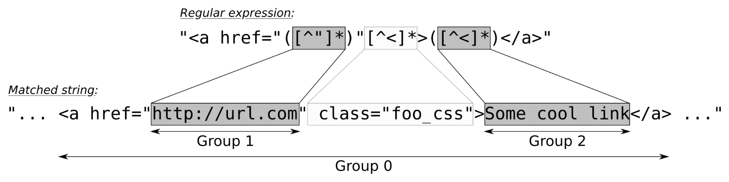
The whole match itself is always Group 0. In this case, this is the full <a href ..... </a> string. The quoted href-part that contains the URL being linked to is Group 1. The ( ) parentheses in the regular expression define such a . The other one is the part between the <a ...> and </a>, which contains the link description.
There are various STL functions that accept regex objects, but we directly used a regex token iterator adapter, which is a high-level abstraction that uses std::regex_search under the hood in order to automate recurring matching work. We instantiated it like this:
sregex_token_iterator it {begin(in), end(in), link_re, {1, 2}};
The begin and end part denote our input string over which the regex token iterator shall iterate and match all links. The is, of course, the complex regular expression we implemented to match links. The {1, 2} part is the next complicated looking thing. It instructs the token iterator to stop on each full match and first yield Group 1, then after incrementing the iterator to yield Group 2, and after incrementing it again, it would finally search for the next match in the string. This somewhat intelligent behavior really spares us some code lines.
Let's have a look at another example to make sure we got the idea. Let's imagine the regular expression, "a(b*)(c*)". It will match strings that contain an a character, then none or arbitrarily many b characters, and then none or arbitrarily many c characters:
const string s {" abc abbccc "};
const regex re {"a(b*)(c*)"};
sregex_token_iterator it {begin(s), end(s), re, {1, 2}};
print( *it ); // prints b
++it;
print( *it ); // prints c
++it;
print( *it ); // prints bb
++it;
print( *it ); // prints ccc
There is also the std::regex_iterator class, which emits the substrings that are between regex matches.
In the last recipe, we learned how to format the output with output streams. And while doing the same, we realized two facts:
A lot of people do not like I/O streams for such reasons, and even in C++, they still use printf for formatting their strings.
In this recipe, we will see how to format types on the fly without too much I/O manipulator noise in our code.
We are going to implement a class, format_guard, which can automatically revert any format setting. Additionally, we add a wrapper type, which can contain any value, but when it is printed, it gets special formatting without burdening us with I/O manipulator noise:
#include <iostream>
#include <iomanip>
using namespace std;
class format_guard {
decltype(cout.flags()) f {cout.flags()};
public:
~format_guard() { cout.flags(f); }
};
template <typename T>
struct scientific_type {
T value;
explicit scientific_type(T val) : value{val} {}
};
template <typename T>
ostream& operator<<(ostream &os, const scientific_type<T> &w) {
format_guard _;
os << scientific << uppercase << showpos;
return os << w.value;
}
int main()
{
{
format_guard _;
cout << hex << scientific << showbase << uppercase;
cout << "Numbers with special formatting:n";
cout << 0x123abc << 'n';
cout << 0.123456789 << 'n';
}
cout << "Same numbers, but normal formatting again:n";
cout << 0x123abc << 'n';
cout << 0.123456789 << 'n';
cout << "Mixed formatting: "
<< 123.0 << " "
<< scientific_type{123.0} << " "
<< 123.456 << 'n';
}
$ ./pretty_print_on_the_fly
Numbers with special formatting:
0X123ABC
1.234568E-01
Same numbers, but normal formatting again:
1194684
0.123457
Mixed formatting: 123 +1.230000E+02 123.456
In none of the recipes in this chapter, we used exceptions to catch errors. While this is certainly possible, working on stream objects without exceptions is already very convenient. If we try to parse in 10 values, but this fails somewhere in the middle, the whole stream object sets itself into a fail state and stops further parsing. This way, we do not run into the danger of parsing variables from the wrong offset in the stream. We can just do the parsing in a conditional, such as if (cin >> foo >> bar >> ...). If this fails, we handle it. It does not appear very advantageous to embrace parsing in a try { ... } catch ... block.
In fact, the C++ I/O stream library already existed before there were exceptions in C++. Exception support was added later, which might be an explanation why they are not a first-class supported feature in the stream library.
In order to use exceptions in the stream library, we must configure each stream object individually to throw an exception, whenever it sets itself into a fail state. Unfortunately, the error explanations in the exception objects, which we can then catch later, are not thoroughly standardized. This leads to not really helpful error messages, as we will see in this section. If we really want to use exceptions with stream objects, we can additionally poll the C library for filesystem error states to get some additional information.
In this section, we are going to write a program that can fail in different ways, handle those with exceptions, and see how to squeeze more information out of those afterward.
We will implement a program that opens a file (which might fail), and then we'll read an integer out of it (which might fail, too). We do this with activated exceptions and then we see how we can handle those:
#include <iostream>
#include <fstream>
#include <system_error>
#include <cstring>
using namespace std;
int main()
{
ifstream f;
f.exceptions(f.failbit | f.badbit);
try {
f.open("non_existant.txt");
int i;
f >> i;
cout << "integer has value: " << i << 'n';
}
catch (ios_base::failure& e) {
cerr << "Caught error: ";
if (errno) {
cerr << strerror(errno) << 'n';
} else {
cerr << e.what() << 'n';
}
}
}
$ ./readable_error_msg
Caught error: ios_base::clear: unspecified iostream_category error
$ ./readable_error_msg
Caught error: No such file or directory
We have seen that we can enable exceptions per stream object, s, with s.exceptions(s.failbit | s.badbit). This means, that there is no way to use, for example, the std::ifstream instance's constructor for opening a file if we want to get an exception when opening that file is not possible:
ifstream f {"non_existant.txt"};
f.exceptions(...); // too late for an exception
This is a pity because exceptions actually promise that they make error handling less clumsy compared to old-school C-style code, which is riddled with loads of if branches, which handle errors after every step.
If we played around trying to provoke various reasons for streams to fail, we would realize that there are no different exceptions being thrown. This way, we can only find out when we get an error, but not what specific error (This is, of course, not true for exception handling in general, but for the STL stream library). That is why we additionally consulted the value of errno. This global variable is an ancient construct, which has already been used in the old days when there were no C++ or exceptions in general.
If any system-related function has seen an error condition, it is able to set the errno variable to something other than 0 (0 describes the absence of errors), and then the caller is able to read that error number and look up what its value means. The only problem with this is that when we have a multithreaded application, and all the threads use functions that can set this error variable, whose error value is it? If we read it even though there is no error, it could carry an error value because some other system function running in a different thread may have experienced an error. Luckily, this flaw has been gone since C++11, where every thread in a process sees its own errno variable.
Without elaborating the ups and downs of an ancient error indication method, it can give us useful extra information when an exception is triggered on system-based things such as file streams. Exceptions tell us when it happened, and errno can tell us what happened if it happened at the system level.
In this chapter, we will cover the following recipes:
This chapter is dedicated to utility classes that are very useful for solving very specific tasks. Some of them are indeed so useful that we will most probably see them extremely often in any C++ program snippet in the future or have at least already seen them sprinkled over all other chapters in this book.
The first two recipes are about measuring and taking the time. We will also see how to convert between different time units and how to jump between points in time.
Then, we will have a look at the optional, variant, and any types (which all came with C++14 and C++17) as well as some tuple tricks in another five recipes.
Since C++11, we also got sophisticated smart pointer types, namely unique_ptr, shared_ptr, and weak_ptr, which are an enormously effective help regarding memory management, which is why we will have a dedicated look at them in five recipes.
Finally, we will have a panoramic view of the library parts of the STL that are about generating random numbers. Apart from learning about the most important characteristics of the STL's random engines, we will also learn how to apply shaping to random numbers in order to get distributions that fit our actual needs.
Since C++11, the STL contains some new types and functions for taking, measuring, and displaying time. This part of the library exists in the std::chrono namespace and has some sophisticated details.
In this recipe, we will concentrate on measuring time spans and how to convert the result of the measurement between units, such as seconds, milliseconds, and microseconds. The STL provides facilities, which enable us to define our own time units and convert between them seamlessly.
In this section, we will write a little game that prompts the user to enter a specific word. The time that the user needs to type this word into the keyboard is measured and displayed in multiple time units:
#include <iostream>
#include <chrono>
#include <ratio>
#include <cmath>
#include <iomanip>
#include <optional>
using namespace std;
using seconds = chrono::duration<double>;
using milliseconds = chrono::duration<
double, ratio_multiply<seconds::period, milli>>;
using microseconds = chrono::duration<
double, ratio_multiply<seconds::period, micro>>;
static pair<string, seconds> get_input()
{
string s;
const auto tic (chrono::steady_clock::now());
if (!(cin >> s)) {
return {{}, {}};
}
const auto toc (chrono::steady_clock::now());
return {s, toc - tic};
}
int main()
{
while (true) {
cout << "Please type the word "C++17" as"
" fast as you can.n> ";
const auto [user_input, diff] = get_input();
if (user_input == "") { break; }
if (user_input == "C++17") {
cout << "Bravo. You did it in:n"
<< fixed << setprecision(2)
<< setw(12) << diff.count()
<< " seconds.n"
<< setw(12) << milliseconds(diff).count()
<< " milliseconds.n"
<< setw(12) << microseconds(diff).count()
<< " microseconds.n";
break;
} else {
cout << "Sorry, your input does not match."
" You may try again.n";
}
}
}
$ ./ratio_conversion
Please type the word "C++17" as fast as you can.
> c+17
Sorry, your input does not match. You may try again.
Please type the word "C++17" as fast as you can.
> C++17
Bravo. You did it in:
1.48 seconds.
1480.10 milliseconds.
1480099.00 microseconds.
While this section is all about converting between different time units, we first had to choose one of the three available clock objects. There is generally the choice between system_clock, steady_clock, and high_resolution_clock in the std::chrono namespace. What are the differences between them? Let's have a closer look:
| Clock | Characteristics |
| system_clock | This represents the system-wide real-time "wall" clock. It is the right choice if we want to obtain the local time. |
| steady_clock | This clock is promised to be monotonic. This means that it will never be set back by any amount of time. This can happen to other clocks when their time is corrected by minimal amounts, or even when the time is switched between winter and summer time. |
| high_resolution_clock | This is the clock with the most fine-grained clock tick period the STL implementation can provide. |
Since we measured the time distance, or duration from one absolute point in time and the other absolute point in time (which we captured in the variables tic and toc), we are not interested if those points in time were globally skewed. Even if the clock was 112 years, 5 hours, 10 minutes, and 1 second (or whatever) late or ahead of time, then this does not make a difference on the difference between them. The only important thing is that after we save the time point tic and before we save the time point toc, the clock must not be micro-adjusted (which happens on many systems from time to time) because that would distort our measurement. For these requirements, steady_clock is the optimal choice. Its implementation can be based on the processor's timestamp counter, which always counts up monotonously since the system was started.
Okay, now with the right time object choice, we are able to save points in time via chrono::steady_clock::now(). The now function returns us a chrono::time_point<chrono::steady_clock> typed value. The difference between two such values (as in toc - tic) is a time span, or duration of type chrono::duration. As this is the central type of this section, this gets a little complicated now. Let's have a closer look at the template type interface of duration:
template<
class Rep,
class Period = std::ratio<1>
> class duration;
The parameters we can change are called Rep and Period. Rep is easy to explain: this is just the numeric variable type that is used to save the time value. For the existing STL time units, this is usually long long int. In this recipe, we chose double. Because of our choice, we can save time values in seconds by default and then convert them to milli- or microseconds. If we save the time duration of 1.2345 seconds in the chrono::seconds type, then it would be rounded to one full second. This way, we would have to save the time difference between tic and toc in chrono::microseconds and could then convert to less-fine-grained units. With our double choice for Rep, we can convert up and down and lose only a minimal amount of precision, which does not hurt in this example.
We used Rep = double for all our time units, so they differed only in our choice of the Period parameter:
using seconds = chrono::duration<double>;
using milliseconds = chrono::duration<double,
ratio_multiply<seconds::period, milli>>;
using microseconds = chrono::duration<double,
ratio_multiply<seconds::period, micro>>;
While seconds is the simplest unit to describe, as it works with Period = ratio<1>, the others have to be adjusted. As one millisecond is a thousandth of a second, we multiply the seconds::period (which is just a getter function to the Period parameter) with milli, which is a type alias for std::ratio<1, 1000> (std::ratio<a, b> represents the fractional value a/b). The ratio_multiply type is basically a compile time function, which represents the type that results from multiplying one ratio type with another.
Maybe this sounds too complicated, so let's have a look at an example: ratio_multiply<ratio<2, 3>, ratio<4, 5>> results in ratio<8, 15> because (2/3) * (4/5) = 8/15.
Our resulting type definitions are equivalent to the following definitions:
using seconds = chrono::duration<double, ratio<1, 1>>;
using milliseconds = chrono::duration<double, ratio<1, 1000>>;
using microseconds = chrono::duration<double, ratio<1, 1000000>>;
Having these types lined up, it is easy to convert between them. If we have a time duration d of type seconds, we can transform it to milliseconds just by feeding it through the constructor of the other type, that is, milliseconds(d).
In other tutorials or books, you might run across duration_cast whenever time durations are transformed. If we have a duration value of type chrono::milliseconds and want to transform it to chrono::hours, for example, we do indeed need to write duration_cast<chrono::hours>(milliseconds_value) because these units depend on integer types. Transforming from fine-grained units to less-fine-grained units leads to precision loss in that case, which is why we need a duration_cast. For double- or float-based duration units, this is not needed.
Until C++11, it was quite a hassle to take the wall clock time and just print it, because C++ did not have its own time library. It was always necessary to call functions of the C library, which looks very archaic, considering that such calls could be encapsulated nicely into their own classes.
Since C++11, the STL provides the chrono library, which makes time-related tasks much easier to implement.
In this recipe, we are going to take the local time, print it, and play around by adding different time offsets, which is a really comfortable thing to do with std::chrono.
We are going to save the current time and print it. Additionally, our program will add different offsets to the saved time point and print the resulting time points too:
#include <iostream>
#include <iomanip>
#include <chrono>
using namespace std;
ostream& operator<<(ostream &os,
const chrono::time_point<chrono::system_clock> &t)
{
const auto tt (chrono::system_clock::to_time_t(t));
const auto loct (std::localtime(&tt));
return os << put_time(loct, "%c");
}
using days = chrono::duration<
chrono::hours::rep,
ratio_multiply<chrono::hours::period, ratio<24>>>;
constexpr days operator ""_days(unsigned long long h)
{
return days{h};
}
int main()
{
auto now (chrono::system_clock::now());
cout << "The current date and time is " << now << 'n';
chrono::hours chrono_12h {12};
cout << "In 12 hours, it will be "
<< (now + chrono_12h)<< 'n';
using namespace chrono_literals;
cout << "12 hours and 15 minutes ago, it was "
<< (now - 12h - 15min) << 'n'
<< "1 week ago, it was "
<< (now - 7_days) << 'n';
}
$ ./relative_absolute_times
The current date and time is Fri May 5 13:20:38 2017
In 12 hours, it will be Sat May 6 01:20:38 2017
12 hours and 15 minutes ago, it was Fri May 5 01:05:38 2017
1 week ago, it was Fri Apr 28 13:20:38 2017
We obtained the current time point from std::chrono::system_clock. This STL clock class is the only one that can transform its time point values to a time structure that can be displayed as a human-readable time description string.
In order to print such time points, we implemented operator<< for output streams:
ostream& operator<<(ostream &os,
const chrono::time_point<chrono::system_clock> &t)
{
const auto tt (chrono::system_clock::to_time_t(t));
const auto loct (std::localtime(&tt));
return os << put_time(loct, "%c");
}
What happens here first, is that we transform from chrono::time_point<chrono::system_clock> to std::time_t. Values of this type can be transformed to a local wall clock relevant time value, which we do with std::localtime. This function returns us a pointer to a converted value (don't worry about the maintenance of the memory behind this pointer; it is a static object not allocated on the heap), which we can now finally print.
The std::put_time function accepts such an object together with a time format string. "%c" displays a standard date-time string, such as Sun Mar 12 11:33:40 2017. We could also have written "%m/%d/%y"; then the program would have printed the time in the format, 03/12/17. The whole list of existing format string modifiers for time is very long, but it is nicely documented to its full extent in the online C++ reference.
Aside from printing, we also added time offsets to our time point. This is very easy because we can express time durations, such as 12 hours and 15 minutes as 12h + 15min. The chrono_literals namespace already provides handy type literals for hours (h), minutes (min), seconds (s), milliseconds (ms), microseconds (us), and nanoseconds (ns).
Adding such a duration value to a time point value creates a new time point value because these types have the right operator+ and operator- overloads, which is why it is so simple to add and display offsets in time.
When a program communicates with the outside world and relies on values it gets from there, then all kinds of failures can happen.
This means that whenever we write a function that ought to return a value, but that can also possibly fail, then this must be reflected in some change of the function interface. We have several possibilities. Let's see how we can design the interface of a function that will return a string, but that could also fail:
All these approaches have different advantages and disadvantages. Since C++17, there is a new type that can be used to solve such a problem in a different way: std::optional. The notion of an optional value comes from purely functional programming languages (where they are sometimes called Maybe types) and can lead to very elegant code.
We can wrap optional around our own types in order to signal empty or erroneous values. In this recipe, we will learn how to do that.
In this section, we will implement a program that reads integers from the user and sums them up. Because the user can always input random things instead of numbers, we will see how optional can improve our error handling:
#include <iostream>
#include <optional>
using namespace std;
using oint = optional<int>;
oint read_int()
{
int i;
if (cin >> i) { return {i}; }
return {};
}
oint operator+(oint a, oint b)
{
if (!a || !b) { return {}; }
return {*a + *b};
}
oint operator+(oint a, int b)
{
if (!a) { return {}; }
return {*a + b};
}
int main()
{
cout << "Please enter 2 integers.n> ";
auto a {read_int()};
auto b {read_int()};
auto sum (a + b + 10);
if (sum) {
cout << *a << " + " << *b << " + 10 = "
<< *sum << 'n';
} else {
cout << "sorry, the input was "
"something else than 2 numbers.n";
}
}
$ ./optional
Please enter 2 integers.
> 1 2
1 + 2 + 10 = 13
$ ./optional
Please enter 2 integers.
> 2 z
sorry, the input was something else than 2 numbers.
Working with optional is generally very simple and convenient. If we want to attach the notion of possible failure or optionality to any type T, we can just wrap it into std::optional<T> and that's it.
Whenever we get such a value from somewhere, we have to check whether it is in the empty state or whether it contains a real value. The bool optional::has_value() function does that for us. If it returns true, we may access the value. Accessing the value of an optional can be done with T& optional::value().
Instead of always writing if (x.has_value()) {...} and x.value(), we can also write if (x) {...} and *x. The std::optional type defines explicit conversion to bool and operator* in such a way that dealing with an optional type is similar to dealing with a pointer.
Another handy operator helper that is good to know is the operator-> overload of optional. If we have a struct Foo { int a; string b; } type and want to access one of its members through an optional<Foo> variable, x, then we can write x->a or x->b. Of course, we should first check whether x actually has a value.
If we try to access an optional value even though it does not have a value, then it will throw std::logic_error. This way, it is possible to mess around with a lot of optional values without always checking them. Using a try-catch clause, we could write code in the following form:
cout << "Please enter 3 numbers:n";
try {
cout << "Sum: "
<< (*read_int() + *read_int() + *read_int())
<< 'n';
} catch (const std::bad_optional_access &) {
cout << "Unfortunately you did not enter 3 numbersn";
}
Another gimmick of std::optional is optional::value_or. If we want to take an optional's value and fall back to a default value if it is in the empty state, then this is of help. x = optional_var.value_or(123) does this job in one concise line, where 123 is the fallback default value.
Since C++11, the STL provides std::tuple. This type allows us to sporadically bundle multiple values into a single variable and reach them around. The notion of tuples has been there for a long time in a lot of programming languages, and some recipes in this book are already devoted to this type because it is extremely versatile to use.
However, we sometimes end up with values bundled up in a tuple and then need to call functions with their individual members. Unpacking the members individually for every function argument is very tedious (and error-prone if we introduce a typo somewhere). The tedious form looks like this: func(get<0>(tup), get<1>(tup), get<2>(tup), ...);.
In this recipe, you will learn how to pack and unpack values to and from tuples in an elegant way, in order to call some functions that don't know about tuples.
We are going to implement a program that packs and unpacks values to and from tuples. Then, we will see how to call functions that know nothing about tuples with values from tuples:
#include <iostream>
#include <iomanip>
#include <tuple>
#include <functional>
#include <string>
#include <list>
using namespace std;
static void print_student(size_t id, const string &name, double gpa)
{
cout << "Student " << quoted(name)
<< ", ID: " << id
<< ", GPA: " << gpa << 'n';
}
int main()
{
using student = tuple<size_t, string, double>;
student john {123, "John Doe"s, 3.7};
{
const auto &[id, name, gpa] = john;
print_student(id, name, gpa);
}
cout << "-----n";
auto arguments_for_later = {
make_tuple(234, "John Doe"s, 3.7),
make_tuple(345, "Billy Foo"s, 4.0),
make_tuple(456, "Cathy Bar"s, 3.5),
};
for (const auto &[id, name, gpa] : arguments_for_later) {
print_student(id, name, gpa);
}
cout << "-----n";
apply(print_student, john);
cout << "-----n";
for (const auto &args : arguments_for_later) {
apply(print_student, args);
}
cout << "-----n";
}
$ ./apply_functions_on_tuples
Student "John Doe", ID: 123, GPA: 3.7
-----
Student "John Doe", ID: 234, GPA: 3.7
Student "Billy Foo", ID: 345, GPA: 4
Student "Cathy Bar", ID: 456, GPA: 3.5
-----
Student "John Doe", ID: 123, GPA: 3.7
-----
Student "John Doe", ID: 234, GPA: 3.7
Student "Billy Foo", ID: 345, GPA: 4
Student "Cathy Bar", ID: 456, GPA: 3.5
-----
The std::apply is a compile-time helper that helps us work more agnostic about the types we handle in our code.
Imagine we have a tuple t with the values (123, "abc"s, 456.0). This tuple has the type, tuple<int, string, double>. Additionally, assume that we have a function f with the signature int f(int, string, double) (the types can also be references).
Then, we can write x = apply(f, t), which will result in a function call, x = f(123, "abc"s, 456.0). The apply method does even return to us what f returns.
Let's have a look at a basic use case for tuples that we most probably already know. We can define a structure as follows, in order to just bundle some variables:
struct Foo {
int a;
string b;
float c;
};
Instead of defining a structure as in the preceding example, we can also define a tuple:
using Foo = tuple<int, string, float>;
We can access its items using the index number of the type from the type list. In order to access the first member of a tuple, t, we can use std::get<0>(t) to access the second member we write std::get<1>, and so on. If the index number is too large, then the compiler will even safely error out.
Throughout the book, we have already used the decomposition capabilities of C++17 for tuples. They allow us to decompose a tuple quickly by just writing auto [a, b, c] = some_tuple in order to access its individual items.
Composing and decomposing single data structures are not the only things we can do with tuples. We can also concatenate or split tuples, or do all kinds of magic. In this recipe, we will play around with such capabilities in order to learn how to do it.
In this section, we will write a program that can print any tuple on the fly. In addition to that, we will write a function that can zip tuples together:
#include <iostream>
#include <tuple>
#include <list>
#include <utility>
#include <string>
#include <iterator>
#include <numeric>
#include <algorithm>
using namespace std;
template <typename T, typename ... Ts>
void print_args(ostream &os, const T &v, const Ts &...vs)
{
os << v;
(void)initializer_list<int>{((os << ", " << vs), 0)...};
}
template <typename ... Ts>
ostream& operator<<(ostream &os, const tuple<Ts...> &t)
{
auto print_to_os ([&os](const auto &...xs) {
print_args(os, xs...);
});
os << "(";
apply(print_to_os, t);
return os << ")";
}
template <typename T>
tuple<double, double, double, double>
sum_min_max_avg(const T &range)
{
auto min_max (minmax_element(begin(range), end(range)));
auto sum (accumulate(begin(range), end(range), 0.0));
return {sum, *min_max.first, *min_max.second,
sum / range.size()};
}
template <typename T1, typename T2>
static auto zip(const T1 &a, const T2 &b)
{
auto z ([](auto ...xs) {
return [xs...](auto ...ys) {
return tuple_cat(make_tuple(xs, ys) ...);
};
});
return apply(apply(z, a), b);
}
int main()
{
auto student_desc (make_tuple("ID", "Name", "GPA"));
auto student (make_tuple(123456, "John Doe", 3.7));
cout << student_desc << 'n'
<< student << 'n';
cout << tuple_cat(student_desc, student) << 'n';
auto zipped (zip(student_desc, student));
cout << zipped << 'n';
auto numbers = {0.0, 1.0, 2.0, 3.0, 4.0};
cout << zip(
make_tuple("Sum", "Minimum", "Maximum", "Average"),
sum_min_max_avg(numbers))
<< 'n';
}
$ ./tuple
(ID, Name, GPA)
(123456, John Doe, 3.7)
(ID, Name, GPA, 123456, John Doe, 3.7)
(ID, 123456, Name, John Doe, GPA, 3.7)
(Sum, 10, Minimum, 0, Maximum, 4, Average, 2)
Some of the code in this section is admittedly complicated. We wrote an operator<< implementation for tuples, which looks very complex but supports all kinds of tuples that themselves consist of printable types. Then we implemented the sum_min_max_avg function, which just returns a tuple. Another very complicated thing to get our head around was the function zip.
The easiest part was sum_min_max_avg. The point about it is that when we define a function that returns an instance tuple<Foo, Bar, Baz> f(), we can just write return {foo_instance, bar_instance, baz_instance}; in that function to construct such a tuple. If you have trouble understanding the STL algorithms we used in the sum_min_max_avg function, then you might want to have a look at the Chapter 22, STL Algorithm Basics of this book, where we already had a closer look at them.
The other code was so complicated that we dedicate the specific helpers their own subsections:
Before we even touched operator<< for output streams, we implemented the print_args function. Due to its variadic argument nature, it accepts any number and type of arguments, as long as the first one is an ostream instance:
template <typename T, typename ... Ts>
void print_args(ostream &os, const T &v, const Ts &...vs)
{
os << v;
(void)initializer_list<int>{((os << ", " << vs), 0)...};
}
This function prints the first item, v, and then prints all the other items from the parameter pack, vs. We print the first item individually because we want to have all items interleaved with ", " but we do not want this string leading or trailing the whole list (as in "1, 2, 3, " or ", 1, 2, 3"). We learned about the initializer_list expansion trick in Chapter 21, Lambda Expressions, in the recipe Calling multiple functions with the same input.
Having that function lined up, we have everything we need in order to print tuples. Our operator<< implementation looks as follows:
template <typename ... Ts>
ostream& operator<<(ostream &os, const tuple<Ts...> &t)
{
auto capt_tup ([&os](const auto &...xs) {
print_args(os, xs...);
});
os << "(";
apply(capt_tup, t);
return os << ")";
}
The first thing we do is defining the function object, capt_tup. When we call capt_tup(foo, bar, whatever), this results in the call, print_args(os, foo, bar, whatever). The only thing this function object does is prepend the output stream object os to its variadic list of arguments.
Afterward, we use std::apply in order to unpack all the items from tuple t. If this step looks too complicated, please have a look at the recipe before this one, which is dedicated to demonstrating how std::apply works.
The zip function accepts two tuples, but looks horribly complicated, although it has a very crisp implementation:
template <typename T1, typename T2>
auto zip(const T1 &a, const T2 &b)
{
auto z ([](auto ...xs) {
return [xs...](auto ...ys) {
return tuple_cat(make_tuple(xs, ys) ...);
};
});
return apply(apply(z, a), b);
}
In order to understand this code better, imagine for a moment that the tuple a carries the values, 1, 2, 3, and tuple b carries the values, 'a', 'b', 'c'.
In such a case, calling apply(z, a) leads to a function call z(1, 2, 3), which returns another function object that captures those values, 1, 2, 3, in the parameter pack xs. When this function object is then called with apply(z(1, 2, 3), b), it gets the values, 'a', 'b', 'c', stuffed into the parameter pack, ys. This is basically the same as if we called z(1, 2, 3)('a', 'b', 'c') directly.
Okay, now that we have xs = (1, 2, 3) and ys = ('a', 'b', 'c'), what happens then? The expression tuple_cat(make_tuple(xs, ys) ...) does the following magic; have a look at the diagram:
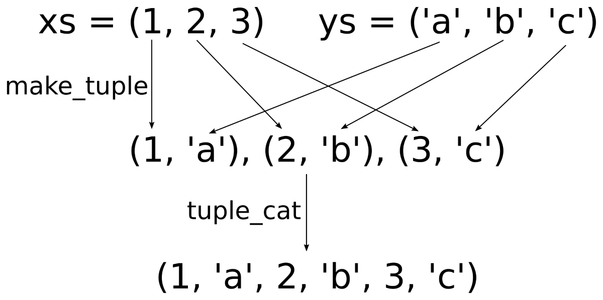
At first, the items from xs and ys are zipped together by interleaving them pairwise. This "pairwise interleaving" happens in the make_tuple(xs, ys) ... expression. This initially only leads to a variadic list of tuples with two items each. In order to get one large tuple, we apply tuple_cat on them and then we finally get a large concatenated tuple that contains all the members of the initial tuples in an interleaved manner.
It can happen that we want to store items of any type in a variable. For such a variable, we then need to be able to check whether it contains anything, and if it does, we need to be able to distinguish what it contains. All this needs to happen in a type-safe manner.
In the past, we were basically able to store pointers to various objects in a void* pointer. A void typed pointer alone cannot tell us what kind of object it points to, so we would need to handcraft some kind of additional mechanism that tells us what to expect. Such code quickly leads to quirky looking and unsafe code.
Another addition of C++17 to the STL is the std::any type. It is designed to hold variables of any kind and provides facilities that enable for type-safe inspection and access to it.
In this recipe, we will play around with this utility type in order to get a feeling of it.
We will implement a function that tries to be able to print everything. It uses std::any as its argument type:
#include <iostream>
#include <iomanip>
#include <list>
#include <any>
#include <iterator>
using namespace std;
using int_list = list<int>;
void print_anything(const std::any &a)
{
if (!a.has_value()) {
cout << "Nothing.n";
} else if (a.type() == typeid(string)) {
cout << "It's a string: "
<< quoted(any_cast<const string&>(a)) << 'n';
} else if (a.type() == typeid(int)) {
cout << "It's an integer: "
<< any_cast<int>(a) << 'n';
} else if (a.type() == typeid(int_list)) {
const auto &l (any_cast<const int_list&>(a));
cout << "It's a list: ";
copy(begin(l), end(l),
ostream_iterator<int>{cout, ", "});
cout << 'n';
} else {
cout << "Can't handle this item.n";
}
}
int main()
{
print_anything({});
print_anything("abc"s);
print_anything(123);
print_anything(int_list{1, 2, 3});
print_anything(any(in_place_type_t<int_list>{}, {1, 2, 3}));
}
$ ./any
Nothing.
It's a string: "abc"
It's an integer: 123
It's a list: 1, 2, 3,
It's a list: 1, 2, 3,
The std::any type is similar in one regard to std::optional--it has a has_value() method that tells if an instance carries a value or not. But apart from that, it can contain literally anything, so it is more complex to handle compared with optional.
Before accessing the content of an any variable, we need to find out what type it carries and, then, cast it to that type.
Finding out if an any instance holds a type T value can be done with a comparison: x.type() == typeid(T). If this comparison results in true, then we can use any_cast to get at the content.
Note that any_cast<T>(x) returns a copy of the internal T value in x. If we want a reference in order to avoid copying of complex objects, we need to use any_cast<T&>(x). This is what we did when we accessed the internal string or list<int> objects in this section's code.
There are not only struct and class primitives in C++ that enable us to compose types. If we want to express that some variable can hold either some type A or a type B (or C, or whatever), we can use union. The problem with unions is that they cannot tell us they were actually initialized to which of the types that they can hold.
Consider the following code:
union U {
int a;
char *b;
float c;
};
void func(U u) { std::cout << u.b << 'n'; }
If we call the func function with a union that was initialized to hold an integer via member a, there is nothing that prevents us from accessing it, as if it was initialized to store a pointer to a string via member b. All kinds of bugs can be spread from such code. Before we start to pack our union with an auxiliary variable that tells us to what it was initialized in order to gain some safety, we can directly use std::variant, which came with C++17.
The variant is kind of the new-school, type-safe, and efficient union type. It does not use the heap, so it is as space-efficient and time-efficient as a union-based handcrafted solution could be, so we do not have to implement it ourselves. It can store anything apart from references, arrays, or the void type.
In this recipe, we will construct an example that profits from variant in order to get a feeling of how to use this cool new addition to the STL.
Let's implement a program that knows the types, cat and dog, and that stores a mixed list of cats and dogs without using any runtime polymorphy:
#include <iostream>
#include <variant>
#include <list>
#include <string>
#include <algorithm>
using namespace std;
class cat {
string name;
public:
cat(string n) : name{n} {}
void meow() const {
cout << name << " says Meow!n";
}
};
class dog {
string name;
public:
dog(string n) : name{n} {}
void woof() const {
cout << name << " says Woof!n";
}
};
using animal = variant<dog, cat>;
template <typename T>
bool is_type(const animal &a) {
return holds_alternative<T>(a);
}
struct animal_voice
{
void operator()(const dog &d) const { d.woof(); }
void operator()(const cat &c) const { c.meow(); }
};
int main()
{
list<animal> l {cat{"Tuba"}, dog{"Balou"}, cat{"Bobby"}};
for (const animal &a : l) {
switch (a.index()) {
case 0:
get<dog>(a).woof();
break;
case 1:
get<cat>(a).meow();
break;
}
}
cout << "-----n";
for (const animal &a : l) {
if (const auto d (get_if<dog>(&a)); d) {
d->woof();
} else if (const auto c (get_if<cat>(&a)); c) {
c->meow();
}
}
cout << "-----n";
for (const animal &a : l) {
visit(animal_voice{}, a);
}
cout << "-----n";
cout << "There are "
<< count_if(begin(l), end(l), is_type<cat>)
<< " cats and "
<< count_if(begin(l), end(l), is_type<dog>)
<< " dogs in the list.n";
}
$ ./variant
Tuba says Meow!
Balou says Woof!
Bobby says Meow!
-----
Tuba says Meow!
Balou says Woof!
Bobby says Meow!
-----
Tuba says Meow!
Balou says Woof!
Bobby says Meow!
-----
There are 2 cats and 1 dogs in the list.
The std::variant type is kind of similar to std::any because both can hold objects of different types, and we need to distinguish at runtime what exactly they hold before we try to access their content.
On the other hand, std::variant is different from std::any in the regard that we must declare what it shall be able to store in the form of a template type list. An instance of std::variant<A, B, C> must hold one instance of type A, B, or C. There is no possibility to hold none of them, which means that std::variant has no notion of optionality.
A variant of type, variant<A, B, C>, mimics a union type that could look like the following:
union U {
A a;
B b;
C c;
};
The problem with unions is that we need to build our own mechanisms to distinguish if it was initialized with an A, B, or C variable. The std::variant type can do this for us without much hassle.
In the code in this section, we used three different ways to handle the content of a variant variable.
The first way was the index() function of variant. For a variant type variant<A, B, C> it can return index 0 if it was initialized to hold an A type, or 1 for B, or 2 for C, and so on for more complex variants.
The next way is the get_if<T> function. It accepts the address of a variant object and returns a T-typed pointer to its content. If the T type is wrong, then this pointer will be a null pointer. It is also possible to call get<T>(x) on a variant variable in order to get a reference to its content, but if that does not succeed, this function throws an exception (before doing such get-casts, checking for the right type can be done with the Boolean predicate holds_alternative<T>(x)).
The last way to access the variant is the std::visit function. It accepts a function object and a variant instance. The visit function then checks of which type the content of the variant is and then calls the right operator() overload of the function object.
For exactly this purpose, we implemented the animal_voice type because it can be used in combination with visit and variant<dog, cat>:
struct animal_voice
{
void operator()(const dog &d) const { d.woof(); }
void operator()(const cat &c) const { c.meow(); }
};
The visit-way of accessing variants can be considered the most elegant one because the code sections that actually access the variant do not need to be hardcoded to the types the variant can hold. This makes our code easier to extend.
Since C++11, the STL provides smart pointers that really help keep track of dynamic memory and its disposal. Even before C++11, there was a class called auto_ptr that was already able to do automatic memory disposal, but it was easy to use the wrong way.
However, with the C++11-generation smart pointers, we seldom need to write new and delete ourselves, which is a really good thing. Smart pointers are a shiny example of automatic memory management. If we maintain dynamically allocated objects with unique_ptr, we are basically safe from memory leaks, because upon its destruction this class automatically calls delete on the object it maintains.
A unique pointer expresses ownership of the object it points to and follows its responsibility of freeing its memory again if it is no longer used. This class has the potential of relieving us forever from memory leaks (at least together with its companions shared_ptr and weak_ptr, but in this recipe, we solely concentrate on unique_ptr). And the best thing is that it imposes no overhead on space and runtime performance, compared with code with raw pointers and manual memory management. (Okay, it still sets its internal raw pointer to nullptr internally after destruction of the object it points to, which cannot always be optimized away. Most manually written code that manages dynamic memory does the same, though.)
In this recipe, we will a look at unique_ptr and how to use it.
We will write a program that shows us how unique_ptr handles memory by creating a custom type that adds some debug messages upon its construction and destruction. Then, we will play around with unique pointers, maintaining dynamically allocated instances of it:
#include <iostream>
#include <memory>
using namespace std;
class Foo
{
public:
string name;
Foo(string n)
: name{move(n)}
{ cout << "CTOR " << name << 'n'; }
~Foo() { cout << "DTOR " << name << 'n'; }
};
void process_item(unique_ptr<Foo> p)
{
if (!p) { return; }
cout << "Processing " << p->name << 'n';
}
int main()
{
{
unique_ptr<Foo> p1 {new Foo{"foo"}};
auto p2 (make_unique<Foo>("bar"));
}
process_item(make_unique<Foo>("foo1"));
auto p1 (make_unique<Foo>("foo2"));
auto p2 (make_unique<Foo>("foo3"));
process_item(move(p1));
cout << "End of main()n";
}
$ ./unique_ptr
CTOR foo
CTOR bar
DTOR bar
DTOR foo
CTOR foo1
Processing foo1
DTOR foo1
CTOR foo2
CTOR foo3
Processing foo2
DTOR foo2
End of main()
DTOR foo3
Handling heap objects with std::unique_ptr is really simple. After we initialized a unique pointer to hold a pointer to some object, there is no way we can accidentally forget about deleting it on some code path.
If we assign some new pointer to a unique pointer, then it will always first delete the old object it pointed to and then store the new pointer. On a unique pointer variable, x, we can also call x.reset() to just delete the object it points to immediately without assigning a new pointer. Another equivalent alternative to reassigning via x = new_pointer is x.reset(new_pointer).
Since pointers need to be checked before they are actually dereferenced, they overload the right operators in a way that enables them to mimic raw pointers. Conditionals like if (p) {...} and if (p != nullptr) {...} perform the same way as we would check a raw pointer.
Dereferencing a unique pointer can be done via the get() function, which returns a raw pointer to the object that can be dereferenced, or directly via operator*, which again mimics raw pointers.
One important characteristic of unique_ptr is that its instances cannot be copied but can be moved from one unique_ptr variable to the other. This is why we had to move an existing unique pointer into the process_item function. If we were able to copy a unique pointer, then this would mean that the object being pointed to is owned by two unique pointers, although this contradicts the design of a unique pointer that is the only owner (and later the "deleter") of the underlying object.
In the last recipe, we learned how to use unique_ptr. This is an enormously useful and important class because it helps us manage dynamically allocated objects. However, it can only handle single ownership. It is not possible to let multiple objects own the same dynamically allocated object because, then, it would be unclear who has to delete it later.
The pointer type, shared_ptr, was designed for specifically this case. Shared pointers can be copied arbitrarily often. An internal reference counting mechanism tracks how many objects are still maintaining a pointer to the payload object. Only the last shared pointer that goes out of scope will call delete on the payload object. This way, we can be sure that we do not get memory leaks because objects are deleted automatically after use. At the same time, we can be sure that they are not deleted too early, or too often (every created object must only be deleted once).
In this recipe, you will learn how to use shared_ptr to automatically manage dynamic objects that are shared between multiple owners and see what's different when comparing it with unique_ptr:
We are going to write a program that is similar to the program we wrote in the unique_ptr recipe in order to get insights into the usage and principles of shared_ptr:
#include <iostream>
#include <memory>
using namespace std;
class Foo
{
public:
string name;
Foo(string n)
: name{move(n)}
{ cout << "CTOR " << name << 'n'; }
~Foo() { cout << "DTOR " << name << 'n'; }
};
void f(shared_ptr<Foo> sp)
{
cout << "f: use counter at "
<< sp.use_count() << 'n';
}
int main()
{
shared_ptr<Foo> fa;
{
cout << "Inner scope beginn";
shared_ptr<Foo> f1 {new Foo{"foo"}};
auto f2 (make_shared<Foo>("bar"));
cout << "f1's use counter at " << f1.use_count() << 'n';
fa = f1;
cout << "f1's use counter at " << f1.use_count() << 'n';
}
cout << "Back to outer scopen";
cout << fa.use_count() << 'n';
cout << "first f() calln";
f(fa);
cout << "second f() calln";
f(move(fa));
cout << "end of main()n";
}
$ ./shared_ptr
Inner scope begin
CTOR foo
CTOR bar
f1's use counter at 1
f1's use counter at 2
DTOR bar
Back to outer scope
1
first f() call
f: use counter at 2
second f() call
f: use counter at 1
DTOR foo
end of main()
When constructing and deleting objects, shared_ptr works basically like unique_ptr. Constructing shared pointers works similarly as creating unique pointers (although there is a function make_shared that creates shared objects as a pendant to unique_ptr pointer's make_unique function).
The major difference from unique_ptr is that we can copy the shared_ptr instances because shared pointers maintain a so-called control block together with the object they manage. The control block contains a pointer to the payload object and a reference counter or use counter. If there are N number of shared_ptr instances pointing to the object, then the use counter also has the value N. Whenever a shared_ptr instance is destructed, then its destructor decrements this internal use counter. The last shared pointer to such an object will hit the condition that it decrements the use counter to 0 during its destruction. This is, then, the shared pointer instance, which calls the delete operator on the payload object! This way, we can't possibly suffer from memory leaks because the object's use count is automatically tracked.
To illustrate this a bit more, let's have a look at the following diagram:
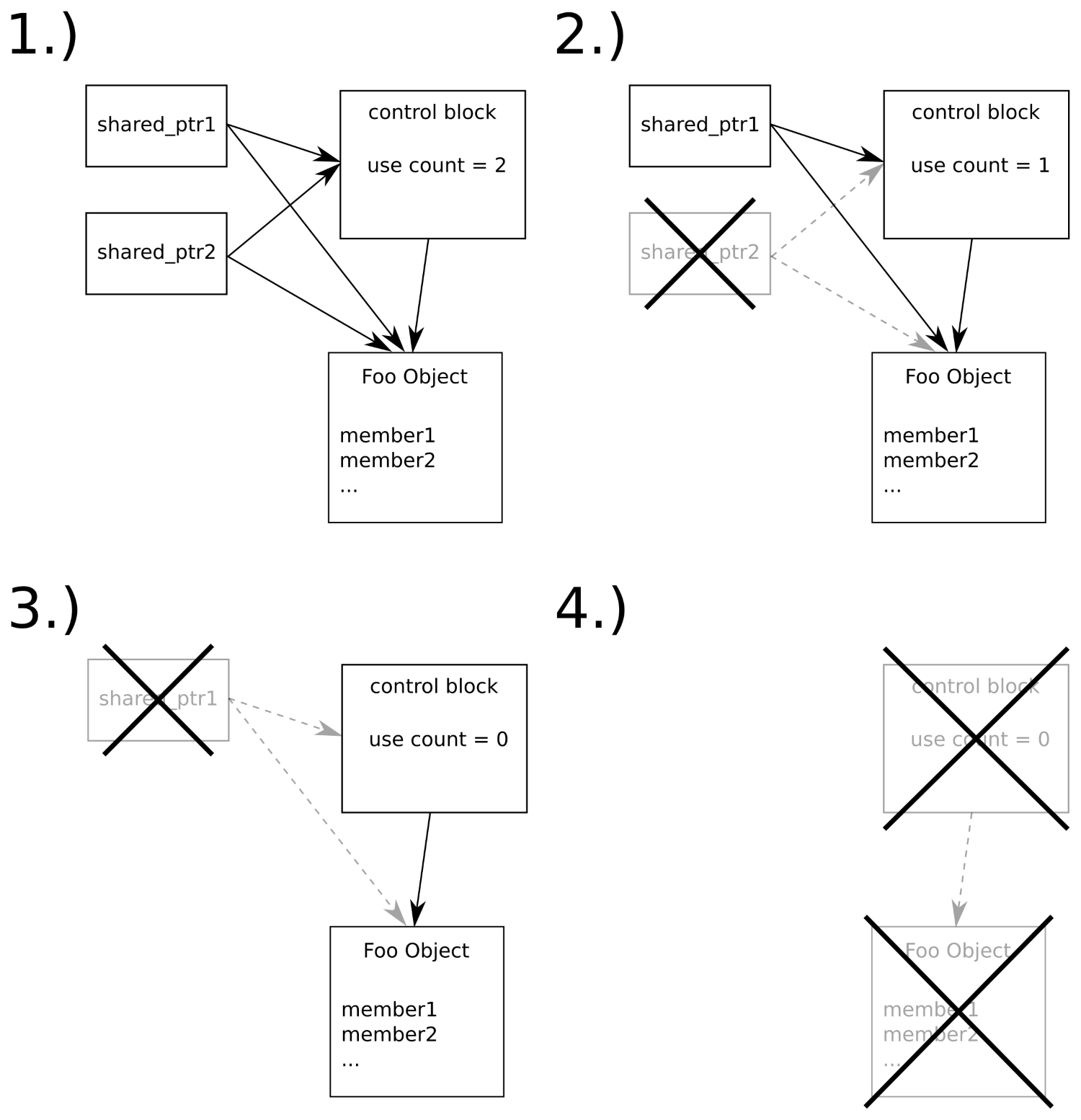
In step 1, we have two shared_ptr instances managing an object of type Foo. The use counter is at value 2. Then, shared_ptr2 is destroyed, which decrements the use counter to 1. The Foo instance is not destroyed yet because there is still the other shared pointer. In step 3, the last shared pointer is destroyed too. This leads to the use counter being decremented to 0. Step 4 happens immediately after step 3. Both the control block and the instance of Foo are destroyed and their memory is released to the heap.
Equipped with shared_ptr and unique_ptr, we can automatically deal with most dynamically allocated objects without having to worry about memory leaks any longer. There is, however, one important caveat to consider--imagine we have two objects on the heap that contain shared pointers to each other, and some other shared pointer points to one of them from somewhere else. If that external shared pointer goes out of scope, then both objects still have the use counters with nonzero values because they reference each other. This leads to a memory leak. Shared pointers should not be used in this case because such cyclic reference chains prevent the use counter of such objects to ever reach 0.
Look at the following code. What if you are told that it contains a potential memory leak?
void function(shared_ptr<A>, shared_ptr<B>, int);
// "function" is defined somewhere else
// ...somewhere later in the code:
function(new A{}, new B{}, other_function());
"Where is the memory leak?", one might ask, since the newly allocated objects A and B are immediately fed into shared_ptr types, and then we are safe from memory leaks.
Yes, it is true that we are safe from memory leaks as soon as the pointers are captured in the shared_ptr instances. The problem is a bit fiddly to grasp.
When we call a function, f(x(), y(), z()), the compiler needs to assemble code that calls x(), y(), and z() first so that it can forward their return values to f. What gets us very bad in combination with the example from before is that the compiler can execute these function calls to x, y, and z in any order.
Looking back at the example, what happens if the compiler decides to structure the code in a way where at first new A{} is called, then other_function(), and then new B{} is called, before the results of these functions are finally fed into function? If other_function() throws an exception, we get a memory leak because we still have an unmanaged object, A, on the heap because we just allocated it but did not have a chance to hand it to the management of shared_ptr. No matter how we catch the exception, the handle to the object is gone and we cannot delete it!
There are two easy ways to circumvent this problem:
// 1.)
function(make_shared<A>(), make_shared<B>(), other_function());
// 2.)
shared_ptr<A> ap {new A{}};
shared_ptr<B> bp {new B{}};
function(ap, bp, other_function());
This way, the objects are already managed by shared_ptr, no matter who throws what exception afterward.
In the recipe about shared_ptr, we learned how useful and easy to use shared pointers are. Together with unique_ptr, they pose an invaluable improvement for code that needs to manage dynamically allocated objects.
Whenever we copy shared_ptr, we increment its internal reference counter. As long as we hold our shared pointer copy, the object being pointed to will not be deleted. But what if we want some kind of weak pointer, which enables us to get at the object as long as it exists but does not prevent its destruction? And how do we determine if the object still exists, then?
In such situations, weak_ptr is our companion. It is a little bit more complicated to use than unique_ptr and shared_ptr, but after following this recipe, we will be ready to use it.
We will implement a program that maintains objects with shared_ptr instances, and then, we mix in weak_ptr to see how this changes the behavior of smart pointer memory handling:
#include <iostream>
#include <iomanip>
#include <memory>
using namespace std;
struct Foo {
int value;
Foo(int i) : value{i} {}
~Foo() { cout << "DTOR Foo " << value << 'n'; }
};
void weak_ptr_info(const weak_ptr<Foo> &p)
{
cout << "---------" << boolalpha
<< "nexpired: " << p.expired()
<< "nuse_count: " << p.use_count()
<< "ncontent: ";
if (const auto sp (p.lock()); sp) {
cout << sp->value << 'n';
} else {
cout << "<null>n";
}
}
int main()
{
weak_ptr<Foo> weak_foo;
weak_ptr_info(weak_foo);
{
auto shared_foo (make_shared<Foo>(1337));
weak_foo = shared_foo;
weak_ptr_info(weak_foo);
}
weak_ptr_info(weak_foo);
}
$ ./weak_ptr
---------
expired: true
use_count: 0
content: <null>
---------
expired: false
use_count: 1
content: 1337
DTOR Foo 1337
---------
expired: true
use_count: 0
content: <null>
Weak pointers provide us a way to point at an object maintained by shared pointers without incrementing its use counter. Okay, a raw pointer could do the same, but a raw pointer cannot tell us if it is dangling or not. A weak pointer can!
In order to understand how weak pointers as an addition to shared pointers work, let's directly jump to an illustrating diagram:
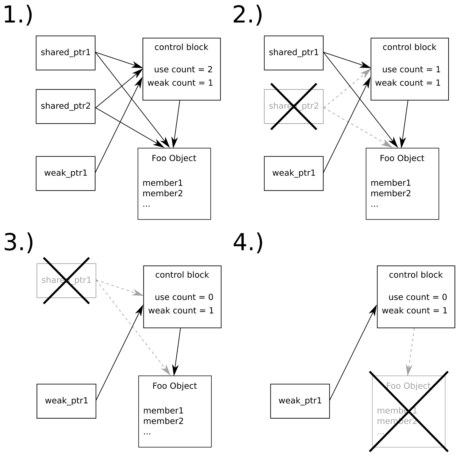
The flow is similar to the diagram in the recipe about shared pointers. In step 1, we have two shared pointers and a weak pointer pointing to the object of type Foo. Although there are three objects pointing to it, only the shared pointers manipulate its use counter, which is why it has the value 2. The weak pointer only manipulates a weak counter of the control block. In steps 2 and 3, the shared pointer instances are destroyed, which leads stepwise to a use counter of 0. In step 4, this results in the Foo object being deleted, but the control block stays there. The weak pointer still needs the control block in order to distinguish if it dangles or not. Only when the last weak pointer that still points to a control block also goes out of scope, the control block is deleted.
We can also say that a dangling weak pointer has expired. In order to check for this attribute, we can ask weak_ptr pointer's expired method, which returns a boolean value. If it is true, then we cannot dereference the weak pointer because there is no object to dereference any longer.
In order to dereference a weak pointer, we need to call lock(). This is safe and convenient because this function returns us a shared pointer. As long as we hold this shared pointer, the object behind it cannot vanish because we incremented the use counter by locking it. If the object is deleted, shortly before the lock() call, then the shared pointer it returns is effectively a null pointer.
Smart pointers (unique_ptr, shared_ptr, and weak_ptr) are extremely useful, and it is, in general, safe to say that a programmer should always use these instead of allocating and freeing memory manually.
But what if objects cannot be allocated using the new operator and/or cannot be freed again using delete? Many legacy libraries come with their own allocation/destruction functions. It seems that this would be a problem because we learned that smart pointers rely on new and delete. If the creation and/or destruction of specific types of objects relies on specific factory functions' deleter interfaces, does this prevent us from getting the humongous benefits of smart pointers?
Not at all. In this recipe, we will see that we only need to perform very minimal customizations on smart pointers in order to let them follow specific procedures for allocation and destruction of specific objects.
In this section, we will define a type that cannot be allocated with new directly and, also, cannot be released again using delete. As this prevents it from being used with smart pointers directly, we perform the necessary little adaptions to instances of unique_ptr and smart_ptr:
#include <iostream>
#include <memory>
#include <string>
using namespace std;
class Foo
{
string name;
Foo(string n)
: name{n}
{ cout << "CTOR " << name << 'n'; }
~Foo() { cout << "DTOR " << name << 'n';}
public:
static Foo* create_foo(string s) {
return new Foo{move(s)};
}
static void destroy_foo(Foo *p) { delete p; }
};
static shared_ptr<Foo> make_shared_foo(string s)
{
return {Foo::create_foo(move(s)), Foo::destroy_foo};
}
static unique_ptr<Foo, void (*)(Foo*)> make_unique_foo(string s)
{
return {Foo::create_foo(move(s)), Foo::destroy_foo};
}
int main()
{
auto ps (make_shared_foo("shared Foo instance"));
auto pu (make_unique_foo("unique Foo instance"));
}
$ ./legacy_shared_ptr
CTOR shared Foo instance
CTOR unique Foo instance
DTOR unique Foo instance
DTOR shared Foo instance
Usually, unique_ptr and shared_ptr just call delete on their internal pointers, whenever they ought to destroy the object they maintain. In this section, we constructed a class which can neither be allocated the C++ way using x = new Foo{123} nor can it be destructed with delete x directly.
The Foo::create_foo function just returns a plain raw pointer to a newly constructed Foo instance, so this causes no further problems because smart pointers work with raw pointers anyway.
The problem we had to deal with is that we need to teach unique_ptr and shared_ptr how to destruct an object if the default way is not the right one.
In that regard, both the smart pointer types differ a little bit. In order to define a custom deleter for unique_ptr, we have to alter its type. Because the type signature of the Foo deleter is void Foo::destroy_foo(Foo*);, the type of the unique_ptr maintaining a Foo instance must be unique_ptr<Foo, void (*)(Foo*)>. Now, it can hold a function pointer to destroy_foo, which we provide it as a second constructor parameter in our make_unique_foo function.
If giving unique_ptr a custom deleter function forces us to change its type, why were we able to do the same with shared_ptr without changing its type? The only thing we had to do there was giving shared_ptr a second constructor parameter, and that's it. Why can't it be as easy for unique_ptr as it is for shared_ptr?
The reason why it is so simple to just provide shared_ptr some kind of callable deleter object without altering the shared pointer's type lies in the nature of shared pointers, which maintain a control block. The control block of shared pointers is an object with virtual functions. This means that the control block of a standard shared pointer compared with the type of a control block of a shared pointer with a custom deleter is different! When we want a unique pointer to use a custom deleter, then this changes the type of the unique pointer. When we want a shared pointer to use a custom deleter, then this changes the type of the internal control block, which is invisible to us because this difference is hidden behind a virtual function interface.
It would be possible to do the same trick with unique pointers, but then, this would imply a certain runtime overhead on them. This is not what we want because unique pointers promise to be completely overhead free at runtime.
Let's imagine we are maintaining a shared pointer to some complex, composed, and dynamically allocated object. Then, we want to start a new thread that does some time-consuming work on a member of this complex object. If we want to release this shared pointer now, the object will be deleted while the other thread is still accessing it. If we don't want to give the thread object the pointer to the whole complex object because that would mess with our nice interface, or for other reasons, does this mean that we have to do manual memory management now?
No. It is possible to use shared pointers that on one hand, point to a member of a large shared object, while on the other hand, perform automatic memory management for the entire initial object.
In this example, we will create such a scenario (without threads to keep it simple) in order to get a feeling for this handy feature of shared_ptr.
We are going to define a structure that is composed of multiple members. Then, we allocate an instance of this structure on the heap that is maintained by a shared pointer. From this shared pointer, we obtain more shared pointers that do not point to the actual object but to its members:
#include <iostream>
#include <memory>
#include <string>
using namespace std;
struct person {
string name;
size_t age;
person(string n, size_t a)
: name{move(n)}, age{a}
{ cout << "CTOR " << name << 'n'; }
~person() { cout << "DTOR " << name << 'n'; }
};
int main()
{
shared_ptr<string> shared_name;
shared_ptr<size_t> shared_age;
{
auto sperson (make_shared<person>("John Doe", 30));
shared_name = shared_ptr<string>(sperson, &sperson->name);
shared_age = shared_ptr<size_t>(sperson, &sperson->age);
}
cout << "name: " << *shared_name
<< "nage: " << *shared_age << 'n';
}
$ ./shared_members
CTOR John Doe
name: John Doe
age: 30
DTOR John Doe
In this section, we first created a shared pointer that manages a dynamically allocated person object. Then we made two other smart pointers point to the person object, but they both did not directly point to the person object itself but instead to its members, name and age.
To summarize what kind of scenario we just created, let's have a look at the following diagram:
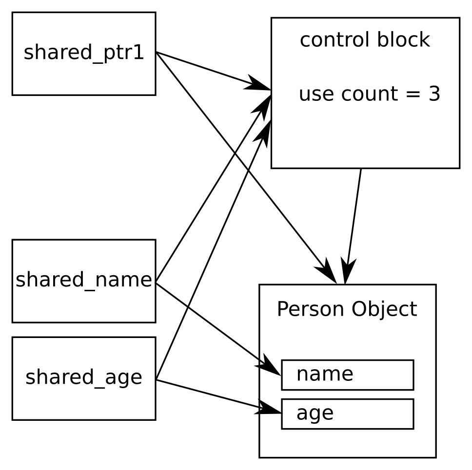
Note that shared_ptr1 points to the person object directly, while shared_name and shared_age point to the name and the age members of the same object. Apparently, they still manage the object's entire lifetime. This is possible because the internal control block pointers still point to the same control block, no matter what sub-object the individual shared pointers point to.
In this scenario, the use count of the control block is 3. This way, the person object is not destroyed when shared_ptr1 is destroyed because the other shared pointers still own the object.
When creating such shared pointer instances that point to members of the shared object, the syntax looks a bit strange. In order to obtain a shared_ptr<string> that points to the name member of a shared person, we need to write the following:
auto sperson (make_shared<person>("John Doe", 30));
auto sname (shared_ptr<string>(sperson, &sperson->name));
In order to get a specific pointer to a member of a shared object, we instantiate a shared pointer with a type specialization of the member we want to access. This is why we write shared_ptr<string>. Then, in the constructor, we first provide the original shared pointer that maintains the person object and, as a second argument, the address of the object the new shared pointer will use when we dereference it.
In order to get random numbers for whatever purpose, C++ programmers usually basically used the rand() function of the C library before C++11. Since C++11, there has been a whole suite of random number generators that serve different purposes and have different characteristics.
These generators are not completely self-explanatory, so we will have a look at all of them in this recipe. In the end, we will see in what ways they differ, how to choose the right one, and that we will most probably never use all of them.
We will implement a procedure that prints a nice illustrating histogram of the numbers a random generator produces. Then, we will run all STL random number generator engines through this procedure and learn from the results. This program contains many repetitive lines, so it might be advantageous to just copy the source code from the code repository accompanying this book on the Internet instead of typing all the repetitive code manually.
#include <iostream>
#include <string>
#include <vector>
#include <random>
#include <iomanip>
#include <limits>
#include <cstdlib>
#include <algorithm>
using namespace std;
template <typename RD>
void histogram(size_t partitions, size_t samples)
{
using rand_t = typename RD::result_type;
partitions = max<size_t>(partitions, 10);
RD rd;
rand_t div ((double(RD::max()) + 1) / partitions);
vector<size_t> v (partitions);
for (size_t i {0}; i < samples; ++i) {
++v[rd() / div];
}
rand_t max_elm (*max_element(begin(v), end(v)));
rand_t max_div (max(max_elm / 100, rand_t(1)));
for (size_t i {0}; i < partitions; ++i) {
cout << setw(2) << i << ": "
<< string(v[i] / max_div, '*') << 'n';
}
}
int main(int argc, char **argv)
{
if (argc != 3) {
cout << "Usage: " << argv[0]
<< " <partitions> <samples>n";
return 1;
}
size_t partitions {stoull(argv[1])};
size_t samples {stoull(argv[2])};
cout << "random_device" << 'n';
histogram<random_device>(partitions, samples);
cout << "ndefault_random_engine" << 'n';
histogram<default_random_engine>(partitions, samples);
cout << "nminstd_rand0" << 'n';
histogram<minstd_rand0>(partitions, samples);
cout << "nminstd_rand" << 'n';
histogram<minstd_rand>(partitions, samples);
cout << "nmt19937" << 'n';
histogram<mt19937>(partitions, samples);
cout << "nmt19937_64" << 'n';
histogram<mt19937_64>(partitions, samples);
cout << "nranlux24_base" << 'n';
histogram<ranlux24_base>(partitions, samples);
cout << "nranlux48_base" << 'n';
histogram<ranlux48_base>(partitions, samples);
cout << "nranlux24" << 'n';
histogram<ranlux24>(partitions, samples);
cout << "nranlux48" << 'n';
histogram<ranlux48>(partitions, samples);
cout << "nknuth_b" << 'n';
histogram<knuth_b>(partitions, samples);
}
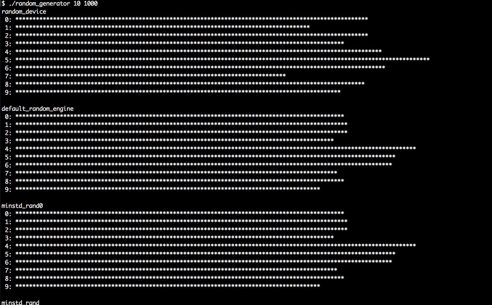
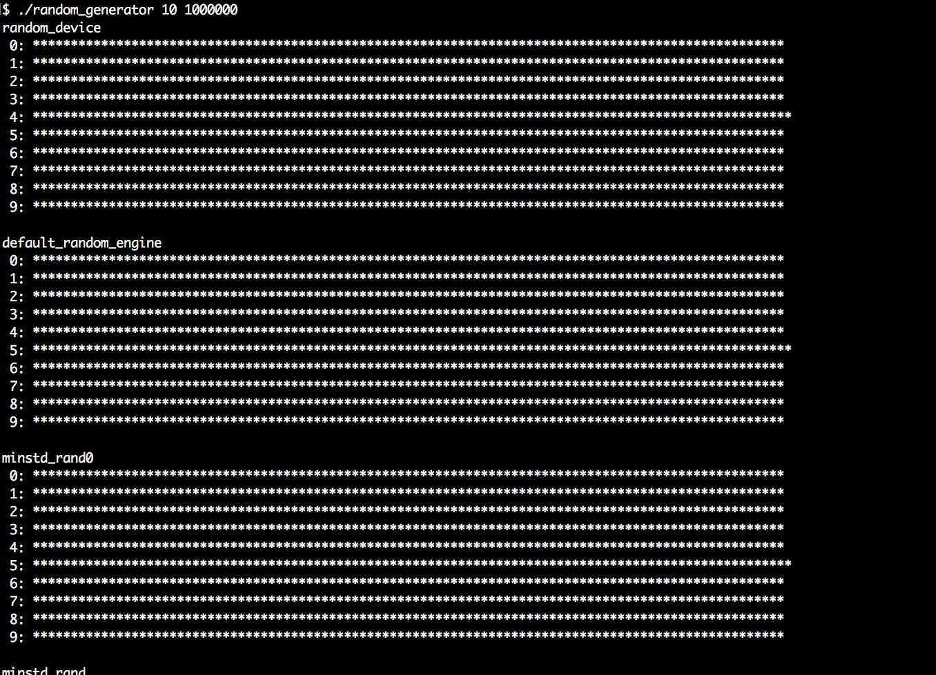
In general, any random number generator needs to be instantiated as an object before use. The resulting object can be called like a function without parameters because it overloads operator(). Every call will then lead to a new random number. It is that simple.
In this section, we wrote a program that is much more complex than that in order to get a bit more information about random number generators. Please play around with the resulting program by launching it with different command-line arguments and realize the following facts:
As we can see, there are a few characteristics to consider. For most standard applications, std::default_random_engine will be completely sufficient. Experts of cryptography or similarly security-sensitive topics will choose wisely between the engines they use, but for us average programmers, this is not too important when we write apps with some randomness.
We should carry home the following three facts from this recipe:
In the last recipe, we learned some bits about the STL random number engines. Generating random numbers this or the other way is often only half of the work.
Another question is, what do we need those numbers for? Are we programmatically "flipping a coin"? People used to do this using rand() % 2, which results in values of 0 and 1 that can then be mapped to head or tail. Fair enough; we do not need a library for that (although randomness experts know that just using the lowest few bits of a random number does not always lead to high-quality random numbers).
What if we want to model a die? Then, we could surely write (rand() % 6) + 1, in order to represent the result after rolling the die. There is still no pressing library needed for such simple tasks.
What if we want to model something that happens with an exact probability of 66%? Okay, then we can come up with a formula like bool yesno = (rand() % 100 > 66). (Oh wait, should it be >=, or is > correct?)
Apart from that, how do we model an unfair die whose sides do not all have the same probability? Or how do we model more complex distributions? Such problems can quickly evolve to scientific tasks. In order to concentrate on our primary problems, let's have a look at what the STL already provides in order to help us.
The STL contains more than a dozen distribution algorithms that can shape random numbers for specific needs. In this recipe, we are going to have a very brief look at all of them, and a closer look at the most generally useful ones.
We are going to generate random numbers, shape them, and print their distribution patterns to the terminal. This way, we can get to know all of them and understand the most important ones, which is useful if we ever need to model something specific with randomness in mind:
#include <iostream>
#include <iomanip>
#include <random>
#include <map>
#include <string>
#include <algorithm>
using namespace std;
template <typename T>
void print_distro(T distro, size_t samples)
{
default_random_engine e;
map<int, size_t> m;
for (size_t i {0}; i < samples; ++i) {
m[distro(e)] += 1;
}
size_t max_elm (max_element(begin(m), end(m),
[](const auto &a, const auto &b) {
return a.second < b.second;
})->second);
size_t max_div (max(max_elm / 100, size_t(1)));
for (const auto [randval, count] : m) {
if (count < max_elm / 200) { continue; }
cout << setw(3) << randval << " : "
<< string(count / max_div, '*') << 'n';
}
}
int main(int argc, char **argv)
{
if (argc != 2) {
cout << "Usage: " << argv[0]
<< " <samples>n";
return 1;
}
size_t samples {stoull(argv[1])};
cout << "uniform_int_distributionn";
print_distro(uniform_int_distribution<int>{0, 9}, samples);
cout << "normal_distributionn";
print_distro(normal_distribution<double>{0.0, 2.0}, samples);
initializer_list<double> intervals {0, 5, 10, 30};
initializer_list<double> weights {0.2, 0.3, 0.5};
cout << "piecewise_constant_distributionn";
print_distro(
piecewise_constant_distribution<double>{
begin(intervals), end(intervals),
begin(weights)},
samples);
cout << "piecewise_linear_distributionn";
initializer_list<double> weights2 {0, 1, 1, 0};
print_distro(
piecewise_linear_distribution<double>{
begin(intervals), end(intervals), begin(weights2)},
samples);
cout << "bernoulli_distributionn";
print_distro(std::bernoulli_distribution{0.75}, samples);
cout << "discrete_distributionn";
print_distro(discrete_distribution<int>{{1, 2, 4, 8}}, samples);
cout << "binomial_distributionn";
print_distro(binomial_distribution<int>{10, 0.3}, samples);
cout << "negative_binomial_distributionn";
print_distro(
negative_binomial_distribution<int>{10, 0.8},
samples);
cout << "geometric_distributionn";
print_distro(geometric_distribution<int>{0.4}, samples);
cout << "exponential_distributionn";
print_distro(exponential_distribution<double>{0.4}, samples);
cout << "gamma_distributionn";
print_distro(gamma_distribution<double>{1.5, 1.0}, samples);
cout << "weibull_distributionn";
print_distro(weibull_distribution<double>{1.5, 1.0}, samples);
cout << "extreme_value_distributionn";
print_distro(
extreme_value_distribution<double>{0.0, 1.0},
samples);
cout << "lognormal_distributionn";
print_distro(lognormal_distribution<double>{0.5, 0.5}, samples);
cout << "chi_squared_distributionn";
print_distro(chi_squared_distribution<double>{1.0}, samples);
cout << "cauchy_distributionn";
print_distro(cauchy_distribution<double>{0.0, 0.1}, samples);
cout << "fisher_f_distributionn";
print_distro(fisher_f_distribution<double>{1.0, 1.0}, samples);
cout << "student_t_distributionn";
print_distro(student_t_distribution<double>{1.0}, samples);
}
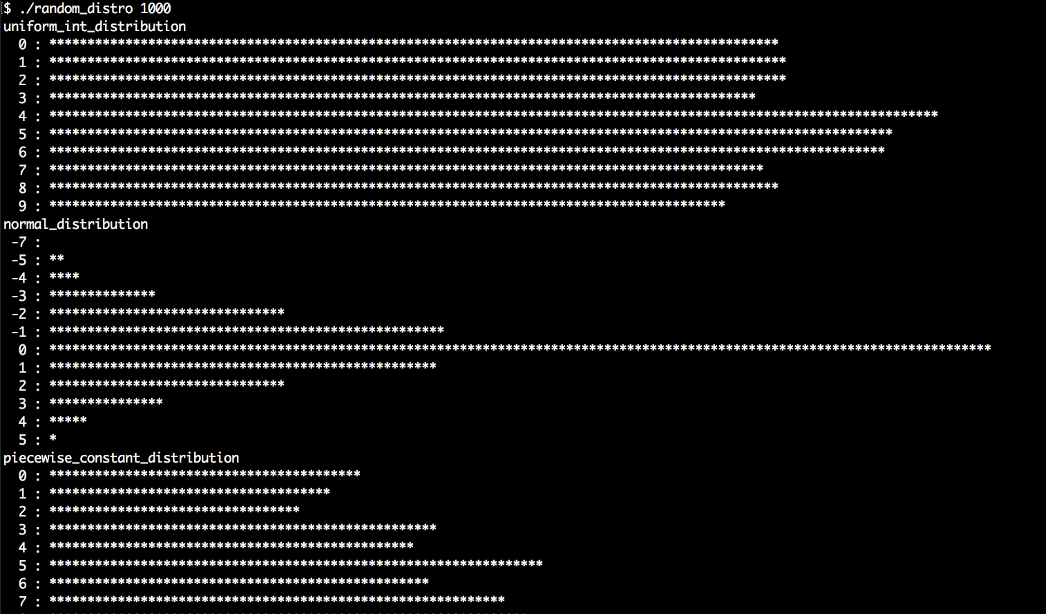
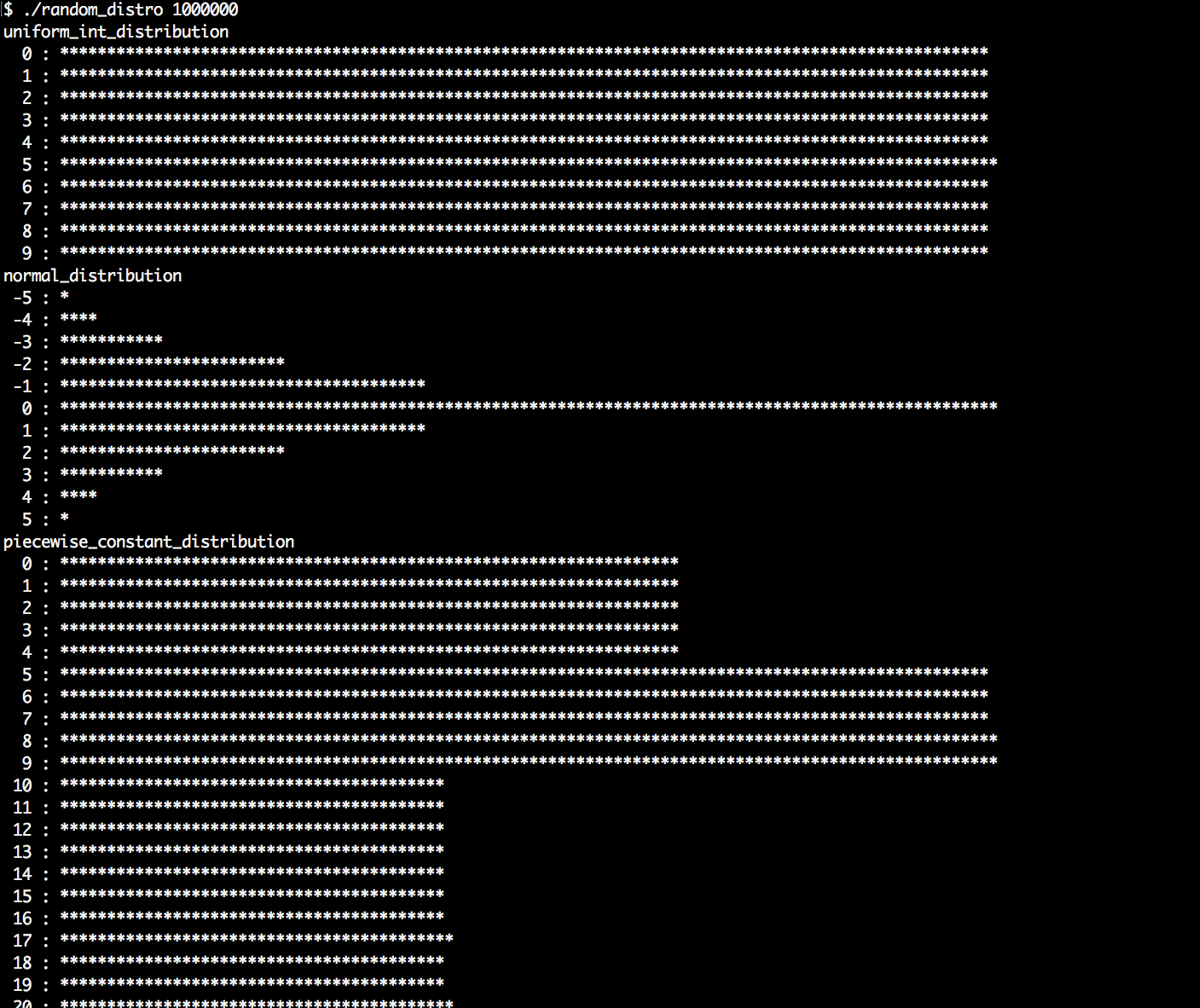
While we usually do not care too much about the random number engine, as long it is fast and produces numbers that are as random as possible, the distribution is something we should choose wisely, depending on the problem we like to solve (or create).
In order to use any distribution, we first need to instantiate a distribution object from it. We have seen that different distributions take different constructor arguments. In the recipe description, we went a bit too briefly over some distribution engines because most of them are too special and/or too complex to cover here. But don't worry, they are all documented in detail in the C++ STL documentation.
However, as soon as we have a distribution instantiated, we can call it like a function that accepts a random engine object as its only parameter. What happens then is that the distribution engine takes a random value from the random engine, applies some magic shaping (which completely depends on the choice of the distribution engine, of course), and then returns us a shaped random value. This leads to completely different histograms, as we saw after executing the program.
The most comprehensive way to get to know the different distributions is playing around with the program we just wrote. In addition to that, let's summarize the most important distributions. For all the distributions that occur in our program but not in the following table, please consult the C++ STL documentation if you are interested:
| Distribution | Description |
| uniform_int_distribution | This distribution accepts a lower and an upper bound value as constructor arguments. It does, then, give us random numbers that always fall into the interval between (including) those bounds. The probability for each of the values in this interval is the same, which gives us a histogram with a flat shape. This distribution is representative of rolling a die, for example, because each side of the die has the same probability to occur. |
| normal_distribution | The normal distribution, or Gauss distribution, occurs practically everywhere in nature. Its STL version accepts a mean value and a standard derivation value as constructor parameters and forms a roof-like shape in the histogram. If we compare the body size or IQ of humans or other animals, or the grades of students, we will realize that these numbers are also normal-distributed. |
| bernoulli_distribution | The Bernoulli distribution is perfect if we want to flip a coin or get a yes/no answer. It emits only the values 0 or 1 and its only constructor parameter is the probability for the value of 1. |
| discrete_distribution | The discrete distribution is interesting if we only want a very limited, discrete set of values for which we want to define the probability for every individual value. Its constructor takes a list of weights and will emit random numbers with probabilities depending on their weight. If we want to model randomly distributed blood groups, of which there are only four different ones that have specific probabilities, then this engine is a perfect match. |
In this chapter, we will cover the following recipes:
Before C++11, C++ didn't have much support for parallelization. This does not mean that starting, controlling, stopping, and synchronizing threads was not possible, but it was necessary to use operating system-specific libraries because threads are inherently operating system-related.
With C++11, we got std::thread, which enables basic portable thread control across all operating systems. For synchronizing threads, C++11 also introduced mutex classes and comfortable RAII-style lock wrappers. In addition to that, std::condition_variable allows for flexible event notification between threads.
Some other really interesting additions are std::async and std::future--we can now wrap arbitrary normal functions into std::async calls in order to execute them asynchronously in the background. Such wrapped functions return std::future objects that promise to contain the result of the function later, so we can do something else before we wait for its arrival.
Another actually enormous improvement to the STL are execution policies, which can be added to 69 of the already existing algorithms. This addition means that we can just add a single execution policy argument to the existing standard algorithm calls in our old programs and get parallelization without complex rewrites.
In this chapter, we will go through all these additions in order to learn the most important things about them. Afterward, we'll have enough oversight of the parallelization support in the C++17 STL. We do not cover all the details, but the most important ones. The overview gained from this book helps in quickly understanding the rest of the parallel programming mechanisms, which you can always look up in the C++ 17 STL documentation online.
Finally, this chapter contains two bonus recipes. In one recipe, we will parallelize the Mandelbrot ASCII renderer from Chapter 23, Advance Use of STL Algorithms, with only minimal changes. In the last recipe, we will implement a tiny library that helps parallelizing complex tasks implicitly and automatically.
C++17 came with one really major extension for parallelism: execution policies for standard algorithms. Sixty nine algorithms were extended to accept execution policies in order to run parallel on multiple cores, and even with enabled vectorization.
For the user, this means that if we already use STL algorithms everywhere, we get a nice parallelization bonus for free. We can easily give our applications subsequent parallelization by simply adding a single execution policy argument to our existing STL algorithm calls.
In this recipe, we will implement a simple program (with a not too serious use case scenario) that lines up multiple STL algorithm calls. While using these, we will see how easy it is to use C++17 execution policies in order to let them run multithreaded. In the last subsections of this section, we will have a closer look at the different execution policies.
In this section, we will write a program that uses some standard algorithms. The program itself is more of an example of how real-life scenarios can look than doing actual real-life work situation. While using these standard algorithms, we are embedding execution policies in order to speed the code up:
#include <iostream>
#include <vector>
#include <random>
#include <algorithm>
#include <execution>
using namespace std;
static bool odd(int n) { return n % 2; }
int main()
{
vector<int> d (50000000);
mt19937 gen;
uniform_int_distribution<int> dis(0, 100000);
auto rand_num ([=] () mutable { return dis(gen); });
generate(execution::par, begin(d), end(d), rand_num);
sort(execution::par, begin(d), end(d));
reverse(execution::par, begin(d), end(d));
auto odds (count_if(execution::par, begin(d), end(d), odd));
cout << (100.0 * odds / d.size())
<< "% of the numbers are odd.n";
}
$ ./auto_parallel
50.4% of the numbers are odd.
Especially since this recipe did not distract us with any complicated real-life problem solution, we were able to fully concentrate on the standard library function calls. It is pretty obvious that the their parallelized versions are hardly different from the classic sequential ones. They only differ by one additional argument, which is the execution policy.
Let's have a look at the invocations and answer three central questions:
generate(execution::par, begin(d), end(d), rand_num);
sort( execution::par, begin(d), end(d));
reverse( execution::par, begin(d), end(d));
auto odds (count_if(execution::par, begin(d), end(d), odd));
Sixty nine of the existing STL algorithms were upgraded to support parallelism in the C++17 standard, and there are seven new ones that also support parallelism. While such an upgrade might be pretty invasive for the implementation, not much has changed in terms of their interface--they all got an additional ExecutionPolicy&& policy argument, and that's it. This does not mean that we always have to provide an execution policy argument. It is just that they additionally support accepting an execution policy as their first argument.
These are the 69 upgraded standard algorithms. There are also the seven new ones that support execution policies from the beginning (highlighted in bold):
|
std::adjacent_difference |
std::inplace_merge |
std::replace_if |
Having these algorithms upgraded is great news! The more our old programs utilize STL algorithms, the easier we can add parallelism to them retroactively. Note that this does not mean that such changes make every program automatically N times faster because multiprogramming is quite a bit more complex than that.
However, instead of designing our own complicated parallel algorithms using std::thread, std::async, or by including external libraries, we can now parallelize standard tasks in a very elegant, operating system-independent way.
The execution policy tells which strategy we allow for the automatic parallelization of our standard algorithm calls.
The following three policy types exist in the std::execution namespace:
| Policy | Meaning |
| sequenced_policy |
The algorithm has to be executed in a sequential form similar to the original algorithm without an execution policy. The globally available instance has the name std::execution::seq. |
| parallel_policy |
The algorithm may be executed with multiple threads that share the work in a parallel fashion. The globally available instance has the name std::execution::par. |
| parallel_unsequenced_policy |
The algorithm may be executed with multiple threads sharing the work. In addition to that, it is permissible to vectorize the code. In this case, container access can be interleaved between threads and also within the same thread due to vectorization. The globally available instance has the name std::execution::par_unseq. |
The execution policies imply specific constraints for us. The stricter the specific constraints, the more parallelization strategy measures we can allow:
As long as we comply with these rules, we should be free from bugs introduced by using the parallel versions of the STL algorithms.
Vectorization is a feature that both the CPU and the compiler need to support. Let's have a quick glance at a simple example to briefly understand what vectorization is and how it works. Imagine we want to sum up numbers from a very large vector. A plain implementation of this task can look like this:
std::vector<int> v {1, 2, 3, 4, 5, 6, 7 /*...*/};
int sum {std::accumulate(v.begin(), v.end(), 0)};
The compiler will eventually generate a loop from the accumulate call, which could look like this:
int sum {0};
for (size_t i {0}; i < v.size(); ++i) {
sum += v[i];
}
Proceeding from this point, with vectorization allowed and enabled, the compiler could then produce the following code. The loop does four accumulation steps in one loop step and also does four times fewer iterations. For the sake of simplicity, the example does not deal with the remainder if the vector does not contain N * 4 elements:
int sum {0};
for (size_t i {0}; i < v.size() / 4; i += 4) {
sum += v[i] + v[i+1] + v[i + 2] + v[i + 3];
}
// if v.size() / 4 has a remainder,
// real code has to deal with that also.
Why should it do this? Many CPUs provide instructions that can perform mathematical operations such as sum += v[i] + v[i+1] + v[i + 2] + v[i + 3]; in just one step. Pressing as many mathematical operations into as few instructions as possible is the target because this speeds up the program.
Automatic vectorization is hard because the compiler needs to understand our program to some degree in order to make our program faster but without tampering with its correctness. At least, we can help the compiler by using standard algorithms as often as possible because those are easier to grasp for the compiler than complicated handcrafted loops with complex data flow dependencies.
A nice and simple possibility to control threads came with C++11. It introduced the this_thread namespace, which includes functions that affect only the caller thread. It contains two different functions that allow putting a thread to sleep for a certain amount of time, so we do not need to use any external or operating system-dependent libraries for such tasks any longer.
In this recipe, we concentrate on how to suspend threads for a certain amount of time, or how to put them to sleep.
We will write a short program that just puts the main thread to sleep for certain amounts of time:
#include <iostream>
#include <chrono>
#include <thread>
using namespace std;
using namespace chrono_literals;
int main()
{
cout << "Going to sleep for 5 seconds"
" and 300 milli seconds.n";
this_thread::sleep_for(5s + 300ms);
cout << "Going to sleep for another 3 seconds.n";
this_thread::sleep_until(
chrono::high_resolution_clock::now() + 3s);
cout << "That's it.n";
}
$ time ./sleep
Going to sleep for 5 seconds and 300 milli seconds.
Going to sleep for another 3 seconds.
That's it.
real 0m8.320s
user 0m0.005s
sys 0m0.003s
The sleep_for and sleep_until functions have been added to C++11 and reside in the std::this_thread namespace. They block the current thread (not the whole process or program) for a specific amount of time. A thread does not consume CPU time while it is blocked. It is just put into an inactive state by the operating system. The operating system does, of course, remind itself of waking the thread up again. The best thing about this is that we do not need to care which operating system our program runs on because the STL abstracts this detail away from us.
The this_thread::sleep_for function accepts a chrono::duration value. In the simplest case, this is just 1s or 5s + 300ms, just like in our example code. In order to get such nice literals for time spans, we need to declare using namespace std::chrono_literals;.
The this_thread::sleep_until function accepts a chrono::time_point instead of a time span. This is comfortable if we wish to put the thread to sleep until some specific wall clock time.
The timing for waking up is only as accurate as the operating system allows. This will be generally accurate enough with most operating systems, but it might become difficult if some application needs nanosecond-granularity.
Another possibility to put a thread to sleep for a short time is this_thread::yield. It accepts no arguments, which means that we cannot know for how long the execution of a thread is placed back. The reason is that this function does not really implement the notion of sleeping or parking a thread. It just tells the operating system in a cooperative way that it can reschedule any other thread of any other process. If there are none, then the thread will be executed again immediately. For this reason, yield is often less useful than just sleeping for a minimal, but specified, amount of time.
Another addition that came with C++11 is the std::thread class. It provides a clean and simple way to start and stop threads, without any need for external libraries or to know how the operating system implements this. It's all just included in the STL.
In this recipe, we will implement a program that starts and stops threads. There are some minor details to know what to do with threads once they are started, so we will go through these too.
We will start multiple threads and see how our program behaves when we unleash multiple processor cores to execute parts of its code at the same time:
#include <iostream>
#include <thread>
using namespace std;
using namespace chrono_literals;
static void thread_with_param(int i)
{
this_thread::sleep_for(1ms * i);
cout << "Hello from thread " << i << 'n';
this_thread::sleep_for(1s * i);
cout << "Bye from thread " << i << 'n';
}
int main()
{
cout << thread::hardware_concurrency()
<< " concurrent threads are supported.n";
thread t1 {thread_with_param, 1};
thread t2 {thread_with_param, 2};
thread t3 {thread_with_param, 3};
t1.join();
t2.join();
t3.detach();
cout << "Threads joined.n";
}
$ ./threads
8 concurrent threads are supported.
Hello from thread 1
Hello from thread 2
Hello from thread 3
Bye from thread 1
Bye from thread 2
Threads joined.
Starting and stopping threads is a very simple thing to do. Multiprogramming starts to be complicated where threads need to work together (sharing resources, waiting for each other, and so on).
In order to start a thread, we first need some function that will be executed by it. The function does not need to be special, as a thread could execute practically every function. Let's pin down a minimal example program that starts a thread and waits for its completion:
void f(int i) { cout << i << 'n'; }
int main()
{
thread t {f, 123};
t.join();
}
The constructor call of std::thread accepts a function pointer or a callable object, followed by arguments that should be used with the function call. It is, of course, also possible to start a thread on a function that doesn't accept any parameters.
If the system has multiple CPU cores, then the threads can run parallel and concurrently. What is the difference between parallel and concurrent? If the computer has only one CPU core, then there can be a lot of threads that run in parallel but never concurrently because one CPU core can only run one thread at a time. The threads are then run in an interleaved way where every thread is executed for some parts of a second, then paused, and then the next thread gets a time slice (for human users, this looks like they run at the same time). If they do not need to share a CPU core, then they can run concurrently, as in really at the same time.
At this point, we have absolutely no control over the following details:
Most operating systems provide possibilities to control also these facets of multiprogramming, but such features are, at this point, not included in the STL.
However, we can start and stop threads and tell them when to work on what and when to pause. That should be enough for a large class of applications. What we did in this section was we started three additional threads. Afterward, we joined most of them and detached the last one. Let's summarize in a simple diagram what happened:
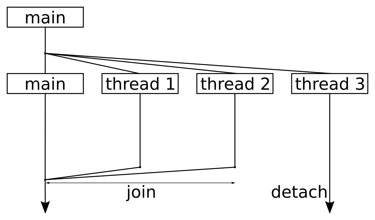
Reading the diagram from top to the bottom, it shows one point in time where we split the program workflow to four threads in total. We started three additional threads that did something (namely waiting and printing), but after starting the threads, the main thread executing the main function remained without work.
Whenever a thread has finished executing the function it was started with, it will return from this function. The standard library then does some tidy up work that results in the thread being removed from the operating system's schedule, and maybe in its destruction, but we do not need to worry about it.
The only thing we need to worry about is joining. When a thread calls function x.join() on another thread object, it is put to sleep until thread x returns. Note that we are out of luck if the thread is trapped in an endless loop! If we want a thread to continue living until it decides to terminate itself, we can call x.detach(). After doing so, we have no external control over the thread any longer. No matter what we decide--we must always join or detach threads. If we don't do one of the two, the destructor of the thread object will call std::terminate(), which leads to an abrupt application shutdown.
The moment when our main function returns, the whole application is, of course, terminated. However, at the same time, our detached thread, t3, was still sleeping before printing its bye message to the terminal. The operating system didn't care--it just terminated our whole program without waiting for that thread to finish. This is something we need to consider. If that additional thread had to complete something important, we would have to make the main function wait for it.
Since the operation of threads is a heavily operating system support-related thing and the STL provides good operating system-agnostic interfaces for that, it is also wise to provide STL support for synchronization between threads. This way, we can not only start and stop threads without external libraries but also synchronize them with abstractions from a single unified library: the STL.
In this recipe, we will have a look at STL mutex classes and RAII lock abstractions. While we play around with some of them in our concrete recipe implementation, we will also get an overview of more synchronization helpers that the STL provides.
We are going to write a program that uses an std::shared_mutex instance in its exclusive and shared modes and to see what that means. Additionally, we do not call the lock and unlock functions ourselves but do the locking with automatic unlocking using RAII helpers:
#include <iostream>
#include <shared_mutex>
#include <thread>
#include <vector>
using namespace std;
using namespace chrono_literals;
shared_mutex shared_mut;
using shrd_lck = shared_lock<shared_mutex>;
using uniq_lck = unique_lock<shared_mutex>;
static void print_exclusive()
{
uniq_lck l {shared_mut, defer_lock};
if (l.try_lock()) {
cout << "Got exclusive lock.n";
} else {
cout << "Unable to lock exclusively.n";
}
}
static void exclusive_throw()
{
uniq_lck l {shared_mut};
throw 123;
}
int main()
{
{
shrd_lck sl1 {shared_mut};
cout << "shared lock once.n";
{
shrd_lck sl2 {shared_mut};
cout << "shared lock twice.n";
print_exclusive();
}
cout << "shared lock once again.n";
print_exclusive();
}
cout << "lock is free.n";
try {
exclusive_throw();
} catch (int e) {
cout << "Got exception " << e << 'n';
}
print_exclusive();
}
$ ./shared_lock
shared lock once.
shared lock twice.
Unable to lock exclusively.
shared lock once again.
Unable to lock exclusively.
lock is free.
Got exception 123
Got exclusive lock.
When looking at the C++ documentation, it is at first a little confusing that there are different mutex classes and RAII lock-helpers. Before looking at our concrete code sample, let us summarize what the STL has available for us.
The term mutex stands for mutual exclusion. In order to prevent that concurrently running threads alter the same object in a non-orchestrated way that might lead to data corruption, we can use mutex objects. The STL provides different mutex classes with different specialties. They all have in common that they have a lock and an unlock method.
Whenever a thread is the first one to call lock() on a mutex that was not locked before, it owns the mutex. At this point, other threads will block on their lock calls, until the first thread calls unlock again. std::mutex can do exactly this.
There are many different mutex classes in the STL:
| Type name | Description |
| mutex |
Standard mutex with a lock and an unlock method. Provides an additional nonblocking try_lock method. |
| timed_mutex |
Same as mutex, but provides additional try_lock_for and try_lock_until methods that allow for timing out instead of blocking forever. |
| recursive_mutex |
Same as mutex, but if a thread locked an instance of it already, it can call lock multiple times on the same mutex object without blocking. It is released after the owning thread called unlock as often as it called lock. |
| recursive_timed_mutex |
Provides the features of both timed_mutex and recursive_mutex. |
| shared_mutex |
This mutex is special in that regard, that it can be locked in exclusive mode and in shared mode. In exclusive mode, it shows the same behavior as the standard mutex class. If a thread locks it in shared mode, it is possible for other threads to lock it in shared mode, too. It will then be unlocked as soon as the last shared mode lock owner releases it. While a lock is locked in shared mode, it is not possible to obtain exclusive ownership. This is very similar to the behavior of shared_ptr, only that it does not manage memory, but lock ownership. |
| shared_timed_mutex |
Combines the features of shared_mutex and timed_mutex for both exclusive and shared mode. |
Everything is nice and easy as long as threads do just lock a mutex, access some concurrence protected object and unlock the mutex again. As soon as a forgetful programmer misses to unlock a mutex somewhere after locking it, or an exception is thrown while a mutex is still locked, things look ugly pretty quick. In the best case, the program just hangs immediately and the missing unlock call is identified quickly. Such bugs, however, are very similar to memory leaks, which also occur when there are missing explicit delete calls.
When regarding memory management, we have unique_ptr, shared_ptr and weak_ptr. Those helpers provide very convenient ways to avoid memory leaks. Such helpers exist for mutexes, too. The simplest one is std::lock_guard. It can be used as follows:
void critical_function()
{
lock_guard<mutex> l {some_mutex};
// critical section
}
lock_guard element's constructor accepts a mutex, on which it calls lock immediately. The whole constructor call will block until it obtains the lock on the mutex. Upon destruction, it unlocks the mutex again. This way it is hard to get the lock/unlock cycle wrong because it happens automatically.
The C++17 STL provides the following different RAII lock-helpers. They all accept a template argument that shall be of the same type as the mutex (although, since C++17, the compiler can deduce that type itself):
| Name | Description |
| lock_guard |
This class provides nothing else than a constructor and a destructor, which lock and unlock a mutex. |
| scoped_lock |
Similar to lock_guard, but supports arbitrarily many mutexes in its constructor. Will release them in opposite order in its destructor. |
| unique_lock |
Locks a mutex in exclusive mode. The constructor also accepts arguments that instruct it to timeout instead of blocking forever on the lock call. It is also possible to not lock the mutex at all, or to assume that it is locked already, or to only try locking the mutex. Additional methods allow to lock and unlock the mutex during the unique_lock lock's lifetime. |
| shared_lock |
Same as unique_lock, but all operations are applied on the mutex in shared mode. |
While lock_guard and scoped_lock have dead-simple interfaces that only consist of constructor and destructor, unique_lock and shared_lock are more complicated, but also more versatile. We will see in later recipes of this chapter, how else they can be used if not for plain simple lock regions.
Let's get back to the recipe code now. Although we only ran the code in single thread context, we have seen how it is meant to use the lock helpers. The shrd_lck type alias stands for shared_lock<shared_mutex> and allows us to lock an instance multiple times in shared mode. As long as sl1 and sl2 exist, no print_exclusive call is able to lock the mutex in exclusive mode. This is still simple.
Now let's get to the exclusively locking functions that came later in the main function:
int main()
{
{
shrd_lck sl1 {shared_mut};
{
shrd_lck sl2 {shared_mut};
print_exclusive();
}
print_exclusive();
}
try {
exclusive_throw();
} catch (int e) {
cout << "Got exception " << e << 'n';
}
print_exclusive();
}
One important detail is that after returning from exclusive_throw, the print_exclusive function is able to lock the mutex again, although exclusive_throw did not exit cleanly due to the exception it throws.
Let's have another look at print_exclusive because it used a strange constructor call:
void print_exclusive()
{
uniq_lck l {shared_mut, defer_lock};
if (l.try_lock()) {
// ...
}
}
We did not only provide shared_mut but also defer_lock as constructor arguments for unique_lock in this procedure. defer_lock is an empty global object that can be used to select a different constructor of unique_lock that simply does not lock the mutex. By doing so, we are able to call l.try_lock() later, which does not block. In case the mutex is locked already, we can do something else. If it was indeed possible to get the lock, we still have the destructor tidying up after us.
If deadlocks had occurred in road traffic, they would have looked like the following situation:

In order to get the traffic flow going again, we either need a large crane that randomly picks one car from the center of the street intersection and removes it. If that is not possible, then we need enough drivers to be cooperative. The deadlock can be solved by all drivers in one direction driving several meters backwards, making space for the other drivers to continue.
In multithreaded programs, such situations, of course, need to be avoided strictly by the programmer. It is however too easy to fail in that regard when the program is really complex.
In this recipe, we are going to write code which intentionally provokes a deadlock situation. Then we will see how to write code that acquires the same resources that led the other code into a deadlock, but use the new STL lock class std::scoped_lock that came with C++17, in order to avoid this mistake.
The code of this section contains two pairs of functions that ought to be executed by concurrent threads, and that acquire two resources in form of mutexes. One pair provokes a deadlock and the other avoids it. In the main function, we are going to try them out:
#include <iostream>
#include <thread>
#include <mutex>
using namespace std;
using namespace chrono_literals;
mutex mut_a;
mutex mut_b;
static void deadlock_func_1()
{
cout << "bad f1 acquiring mutex A..." << endl;
lock_guard<mutex> la {mut_a};
this_thread::sleep_for(100ms);
cout << "bad f1 acquiring mutex B..." << endl;
lock_guard<mutex> lb {mut_b};
cout << "bad f1 got both mutexes." << endl;
}
static void deadlock_func_2()
{
cout << "bad f2 acquiring mutex B..." << endl;
lock_guard<mutex> lb {mut_b};
this_thread::sleep_for(100ms);
cout << "bad f2 acquiring mutex A..." << endl;
lock_guard<mutex> la {mut_a};
cout << "bad f2 got both mutexes." << endl;
}
static void sane_func_1()
{
scoped_lock l {mut_a, mut_b};
cout << "sane f1 got both mutexes." << endl;
}
static void sane_func_2()
{
scoped_lock l {mut_b, mut_a};
cout << "sane f2 got both mutexes." << endl;
}
int main()
{
{
thread t1 {sane_func_1};
thread t2 {sane_func_2};
t1.join();
t2.join();
}
{
thread t1 {deadlock_func_1};
thread t2 {deadlock_func_2};
t1.join();
t2.join();
}
}
$ ./avoid_deadlock
sane f1 got both mutexes
sane f2 got both mutexes
bad f2 acquiring mutex B...
bad f1 acquiring mutex A...
bad f1 acquiring mutex B...
bad f2 acquiring mutex A...
By implementing code that willfully causes a deadlock, we've seen how quick such an unwanted scenario can happen. In a large project, where multiple programmers write code that needs to share a common set of mutex-protected resources, all programmers need to comply with the same order when locking and unlocking mutexes. While such strategies or rules are really easy to follow, they are also easy to forget. Another term for this problem is lock order inversion.
scoped_lock is a real help in such situations. It came with C++17 and works the same way as lock_guard and unique_lock work: its constructor performs the locking, and its destructor the unlocking of a mutex. scoped_lock's specialty is that it can do this with multiple mutexes.
scoped_lock uses the std::lock function, which applies a special algorithm that performs a series of try_lock calls on all the mutexes provided, in order to prevent deadlocking. Therefore it is perfectly safe to use scoped_lock or call std::lock on the same set of locks, but in different orders.
One inconvenience in multithreaded programs is that we must practically secure every data structure they modify, with mutexes or other measures that protect from uncontrolled concurrent modification.
One data structure that is typically used very often for printing is std::cout. If multiple threads access cout concurrently, then the output will appear in interesting mixed patterns on the terminal. In order to prevent this, we would need to write our own function that prints in a concurrency-safe fashion.
We are going to learn how to provide a cout wrapper that consists of minimal code itself and that is as comfortable to use as cout.
In this section, we are going to implement a program that prints to the terminal concurrently from many threads. In order to prevent garbling of the messages due to concurrency, we implement a little helper class that synchronizes printing between threads:
#include <iostream>
#include <thread>
#include <mutex>
#include <sstream>
#include <vector>
using namespace std;
struct pcout : public stringstream {
static inline mutex cout_mutex;
~pcout() {
lock_guard<mutex> l {cout_mutex};
cout << rdbuf();
cout.flush();
}
};
static void print_cout(int id)
{
cout << "cout hello from " << id << 'n';
}
static void print_pcout(int id)
{
pcout{} << "pcout hello from " << id << 'n';
}
int main()
{
vector<thread> v;
for (size_t i {0}; i < 10; ++i) {
v.emplace_back(print_cout, i);
}
for (auto &t : v) { t.join(); }
cout << "=====================n";
v.clear();
for (size_t i {0}; i < 10; ++i) {
v.emplace_back(print_pcout, i);
}
for (auto &t : v) { t.join(); }
}
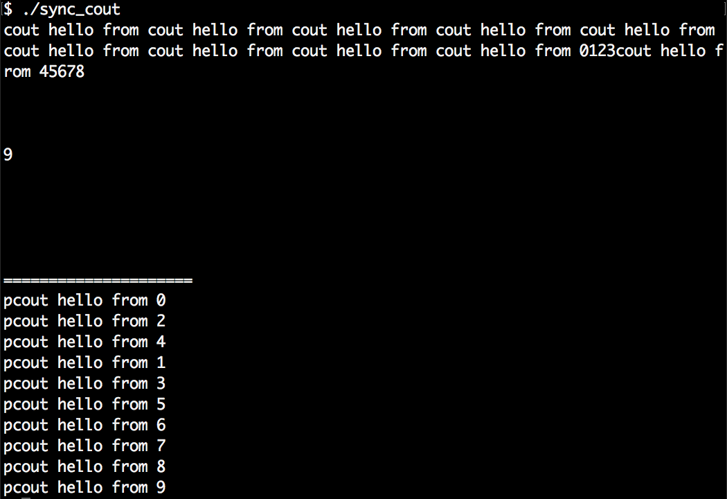
Ok, we've built this "cout wrapper" that automatically serializes concurrent printing attempts. How does it work?
Let's do the same steps our pcout helper does in a manual manner without any magic. First, it instantiates a string stream and accepts the input we feed into it:
stringstream ss;
ss << "This is some printed line " << 123 << 'n';
Then it locks a globally available mutex:
{
lock_guard<mutex> l {cout_mutex};
In this locked scope, it accesses the content of string stream ss, prints it, and releases the mutex again by leaving the scope. The cout.flush() line tells the stream object to print to the terminal immediately. Without this line, a program might run faster because multiple printed lines can be bunched up and printed in a single run later. In our recipes, we will like to see all output lines immediately, so we use the flush method:
cout << ss.rdbuf();
cout.flush();
}
Ok, this is simple enough but tedious to write if we have to to the same thing again and again. We can shorten down the stringstream instantiation as follows:
stringstream{} << "This is some printed line " << 123 << 'n';
This instantiates a string stream object, feeds everything we want to print into it and then destructs it again. The lifetime of the string stream is reduced to just this line. Afterward, we cannot print it any longer, because we cannot access it. Which code is the last that is able to access the stream's content? It is the destructor of stringstream.
We cannot modify stringstream instance's member methods, but we can extend them by wrapping our own type around it via inheritance:
struct pcout : public stringstream {
~pcout() {
lock_guard<mutex> l {cout_mutex};
cout << rdbuf();
cout.flush();
}
};
This class is still a string stream and we can use it like any other string stream. The only difference is that it will lock a mutex and print its own buffer using cout.
We also moved the cout_mutex object into struct pcout as a static instance so we have both bundled in one place.
Sometimes we have specific code sections that can be run in parallel context by multiple threads with the obligation that some setup code must be executed exactly once before executing the actual functions. A simple solution is to just execute the existing setup function before the program enters a state from which parallel code can be executed from time to time.
The drawbacks of such an approach are the following ones:
In this recipe, we will have a look at std::call_once, which is a helper function that solves this problem for us in a simple to use and elegant implicit way.
We are going to write a program that starts multiple threads with exactly the same code. Although they are programmed to execute exactly the same code, our example setup function will only be called once:
#include <iostream>
#include <thread>
#include <mutex>
#include <vector>
using namespace std;
once_flag callflag;
static void once_print()
{
cout << '!';
}
static void print(size_t x)
{
std::call_once(callflag, once_print);
cout << x;
}
int main()
{
vector<thread> v;
for (size_t i {0}; i < 10; ++i) {
v.emplace_back(print, i);
}
for (auto &t : v) { t.join(); }
cout << 'n';
}
$ ./call_once
!1239406758
std:call_once works like a barrier. It maintains access to a function (or a callable object). The first thread to reach it gets to execute the function. Until it has finished, any other thread that reaches the call_once line is blocked. After the first thread returns from the function, all other threads are released, too.
In order to organize this little choreography, a variable is needed from which the other threads can determine if they must wait and when they are released again. This is what our variable once_flag callflag; is for. Every call_once line also needs a once_flag instance as the argument prepending the function that shall be called only once.
Another nice detail is: If it happens, that the thread which is selected to execute the function in call_once fails because some exception is thrown, then the next thread is allowed to execute the function again. This happens in the hope that it will not throw an exception the next time.
Whenever we want some code to be executed in the background, we can simply start a new thread that executes this code. While this happens, we can do something else and then wait for the result. It's simple:
std::thread t {my_function, arg1, arg2, ...};
// do something else
t.join(); // wait for thread to finish
But then the inconvenience starts: t.join() does not give us the return value of my_function. In order to get at that, we need to write a function that calls my_function and stores its return value in some variable that is also accessible for the first thread in which we started the new thread. If such situations occur repeatedly, then this represents quite a bunch of boilerplate code we have to write again and again.
Since C++11, we have std::async which can do exactly this job for us and not only that. In this recipe, we are going to write a simple program that does multiple things at the same time using asynchronous function calls. As std::async is a bit more powerful than that alone, we will have a closer look at its different facets.
We are going to implement a program that does multiple different things concurrently but instead of explicitly starting threads, we use std::async and std::future:
#include <iostream>
#include <iomanip>
#include <map>
#include <string>
#include <algorithm>
#include <iterator>
#include <future>
using namespace std;
static map<char, size_t> histogram(const string &s)
{
map<char, size_t> m;
for (char c : s) { m[c] += 1; }
return m;
}
static string sorted(string s)
{
sort(begin(s), end(s));
return s;
}
static bool is_vowel(char c)
{
char vowels[] {"aeiou"};
return end(vowels) !=
find(begin(vowels), end(vowels), c);
}
static size_t vowels(const string &s)
{
return count_if(begin(s), end(s), is_vowel);
}
int main()
{
cin.unsetf(ios::skipws);
string input {istream_iterator<char>{cin}, {}};
input.pop_back();
auto hist (async(launch::async,
histogram, input));
auto sorted_str (async(launch::async,
sorted, input));
auto vowel_count (async(launch::async,
vowels, input));
for (const auto &[c, count] : hist.get()) {
cout << c << ": " << count << 'n';
}
cout << "Sorted string: "
<< quoted(sorted_str.get()) << 'n'
<< "Total vowels: "
<< vowel_count.get() << 'n';
}
$ echo "foo bar baz foobazinga" | ./async
: 3
a: 4
b: 3
f: 2
g: 1
i: 1
n: 1
o: 4
r: 1
z: 2
Sorted string: " aaaabbbffginoooorzz"
Total vowels: 9
If we would not have used std::async the serial unparallelized code could have looked as simple as that:
auto hist (histogram(input));
auto sorted_str (sorted( input));
auto vowel_count (vowels( input));
for (const auto &[c, count] : hist) {
cout << c << ": " << count << 'n';
}
cout << "Sorted string: " << quoted(sorted_str) << 'n';
cout << "Total vowels: " << vowel_count << 'n';
The only thing we did in order to parallelize the code was the following. We wrapped the three function calls into async(launch::async, ...) calls. This way these three functions are not executed by the main thread we are currently running in. Instead, async starts new threads and lets them execute the functions concurrently. This way we get to execute only the overhead of starting another thread and can continue with the next line of code, while all the work happens in the background:
auto hist (async(launch::async, histogram, input));
auto sorted_str (async(launch::async, sorted, input));
auto vowel_count (async(launch::async, vowels, input));
for (const auto &[c, count] : hist.get()) {
cout << c << ": " << count << 'n';
}
cout << "Sorted string: "
<< quoted(sorted_str.get()) << 'n'
<< "Total vowels: "
<< vowel_count.get() << 'n';
While histogram for example, returns us a map instance, async(..., histogram, ...) does return us a map that was wrapped in a future object before. This future object is kind of an empty placeholder until the thread that executes the histogram function returns. The resulting map is then placed into the future object so we can finally access it. The get function then gives us access to the encapsulated result.
Let's have a look at another minimal example. Consider the following code snippet:
auto x (f(1, 2, 3));
cout << x;
Instead of writing the preceding code, we can also do the following:
auto x (async(launch::async, f, 1, 2, 3));
cout << x.get();
That's basically it. Executing tasks in the background might have never been easier in standard C++. There is still one thing left to resolve: What does launch::async mean? launch::async is a flag that defines the launch policy. There are two policy flags which allow for three constellations:
| Policy choice | Meaning |
| launch::async | The function is guaranteed to be executed by another thread. |
| launch::deferred | The function is executed by the same thread, but later (lazy evaluation). Execution then happens when get or wait is called on the future. If none of both happens, the function is not called at all. |
| launch::async | launch::deferred | Having both flags set, the STL's async implementation is free to choose which policy shall be followed. This is the default choice if no policy is provided. |
There is indeed one last thing we should know about. Suppose, we write code as follows:
async(launch::async, f);
async(launch::async, g);
This might have the motivation of executing functions f and g (we do not care about their return values in this example) in concurrent threads and then doing different things at the same time. While running such code, we will notice that the code blocks on this calls, which is most probably not what we want.
So why does it block? Isn't async all about nonblocking asynchronous calls? Yes it is, but there is one special peculiarity: if a future was obtained from an async call with the launch::async policy, then its destructor performs a blocking wait.
This means that both the async calls from this short example are blocking because the lifetime of the futures they return ends in the same line! We can fix this by capturing their return values in variables with a longer lifetime.
In this recipe, we are going to implement a typical producer/consumer program with multiple threads. The general idea is that there is one thread that produces items and puts them into a queue. Then there is another thread that consumes such items. If there is nothing to produce, the producer thread sleeps. If there is no item in the queue to consume, the consumer sleeps.
Since the queue that both threads have access to is also modified by both whenever an item is produced or consumed, it needs to be protected by a mutex.
Another thing to consider is: What does the consumer do if there is no item in the queue? Does it poll the queue every second until it sees new items? That is not necessary because we can let the consumer wait for wakeup events that are triggered by the producer, whenever there are new items.
C++11 provides a nice data structure called std::condition_variable for this kind of events. In this recipe, we are going to implement a simple producer/consumer app that takes advantage of this.
We are going to implement a simple producer/consumer program which runs a single producer of values in its own thread, as well as a single consumer thread in another thread:
#include <iostream>
#include <queue>
#include <tuple>
#include <condition_variable>
#include <thread>
using namespace std;
using namespace chrono_literals;
queue<size_t> q;
mutex mut;
condition_variable cv;
bool finished {false};
static void producer(size_t items) {
for (size_t i {0}; i < items; ++i) {
this_thread::sleep_for(100ms);
{
lock_guard<mutex> lk {mut};
q.push(i);
}
cv.notify_all();
}
{
lock_guard<mutex> lk {mut};
finished = true;
}
cv.notify_all();
}
static void consumer() {
while (!finished) {
unique_lock<mutex> l {mut};
cv.wait(l, [] { return !q.empty() || finished; });
while (!q.empty()) {
cout << "Got " << q.front()
<< " from queue.n";
q.pop();
}
}
}
int main() {
thread t1 {producer, 10};
thread t2 {consumer};
t1.join();
t2.join();
cout << "finished!n";
}
$ ./producer_consumer
Got 0 from queue.
Got 1 from queue.
Got 2 from queue.
Got 3 from queue.
Got 4 from queue.
Got 5 from queue.
Got 6 from queue.
Got 7 from queue.
Got 8 from queue.
Got 9 from queue.
finished!
In this recipe, we simply started two threads. The first thread produces items and puts them into a queue. The other takes items out of the queue. Whenever one of those threads touches the queue in any way, it locks the common mutex mut which is accessible for both. This way we made sure that it cannot happen that both threads manipulate the queue's state at the same time.
Apart from the queue and the mutex, we declared generally four variables that were involved in the producer-consumer thing:
queue<size_t> q;
mutex mut;
condition_variable cv;
bool finished {false};
The variable finished is easy to explain. It was set to true when the producer finished producing its fixed amount of items. When the consumer sees that this variable is true, it consumes the last items in the queue and stops consuming. But what is the condition_variable cv for? We used cv in two different contexts. One of the contexts was waiting for a specific condition, and the other was signaling that condition.
The consumer side that waits for a specific condition looks like this. The consumer thread loops over a block that first locks mutex mut in a unique_lock. Then it calls cv.wait:
while (!finished) {
unique_lock<mutex> l {mut};
cv.wait(l, [] { return !q.empty() || finished; });
while (!q.empty()) {
// consume
}
}
This code is somewhat equivalent to the following alternative code. We will elaborate soon why it is not really the same:
while (!finished) {
unique_lock<mutex> l {mut};
while (q.empty() && !finished) {
l.unlock();
l.lock();
}
while (!q.empty()) {
// consume
}
}
This means that we generally first acquire the lock and then check what scenario we have:
The real reason why the cv.wait line is not equivalent to the while (q.empty() && ... ) construct is, that we cannot simply loop over a l.unlock(); l.lock(); cycle. If the producer thread is inactive for some time, then this would lead to continuous locking and unlocking of the mutex, which makes no sense because it needlessly burns CPU cycles.
An expression like cv.wait(lock, predicate) will wait until predicate() returns true. But it does not do this by continuously unlocking and locking lock. In order to wake a thread up that blocks on the wait call of a condition_variable object, another thread has to call the notify_one() or notify_all() method on the same object. Only then the waiting thread(s) is/are kicked out of their sleep in order to check if predicate() holds.
The nice thing about the wait call checking the predicate is that if there is a spurious wakeup call, the thread will go to sleep immediately again. This means that it does not really harm the program flow (but maybe the performance) if we have too many notify calls.
On the producer side, we just called cv.notify_all() after the producer inserted an item to the queue and after it produced its last item and set the finished flag to true. This was enough to direct the consumer.
Let's pick up the producer/consumer problem from the last recipe and make it a bit more complicated: We make multiple producers produce items and multiple consumers consume them. In addition to that, we define that the queue shall not exceed a maximum size.
This way not only the consumers have to sleep from time to time if there are no items in the queue, but also the producers have to sleep from time to time when there are enough items in the queue.
We are going to see how to solve this problem with multiple std::condition_variable objects and will also use them in slightly different ways than in the last recipe.
In this section, we are going to implement a program just like in the recipe before, but this time with multiple producers and multiple consumers:
#include <iostream>
#include <iomanip>
#include <sstream>
#include <vector>
#include <queue>
#include <thread>
#include <mutex>
#include <condition_variable>
#include <chrono>
using namespace std;
using namespace chrono_literals;
struct pcout : public stringstream {
static inline mutex cout_mutex;
~pcout() {
lock_guard<mutex> l {cout_mutex};
cout << rdbuf();
}
};
queue<size_t> q;
mutex q_mutex;
bool production_stopped {false};
condition_variable go_produce;
condition_variable go_consume;
static void producer(size_t id, size_t items, size_t stock)
{
for (size_t i = 0; i < items; ++i) {
unique_lock<mutex> lock(q_mutex);
go_produce.wait(lock,
[&] { return q.size() < stock; });
q.push(id * 100 + i);
pcout{} << " Producer " << id << " --> item "
<< setw(3) << q.back() << 'n';
go_consume.notify_all();
this_thread::sleep_for(90ms);
}
pcout{} << "EXIT: Producer " << id << 'n';
}
static void consumer(size_t id)
{
while (!production_stopped || !q.empty()) {
unique_lock<mutex> lock(q_mutex);
if (go_consume.wait_for(lock, 1s,
[] { return !q.empty(); })) {
pcout{} << " item "
<< setw(3) << q.front()
<< " --> Consumer "
<< id << 'n';
q.pop();
go_produce.notify_all();
this_thread::sleep_for(130ms);
}
}
pcout{} << "EXIT: Producer " << id << 'n';
}
int main()
{
vector<thread> workers;
vector<thread> consumers;
for (size_t i = 0; i < 3; ++i) {
workers.emplace_back(producer, i, 15, 5);
}
for (size_t i = 0; i < 5; ++i) {
consumers.emplace_back(consumer, i);
}
for (auto &t : workers) { t.join(); }
production_stopped = true;
for (auto &t : consumers) { t.join(); }
}
$ ./multi_producer_consumer
Producer 0 --> item 0
Producer 1 --> item 100
item 0 --> Consumer 0
Producer 2 --> item 200
item 100 --> Consumer 1
item 200 --> Consumer 2
Producer 0 --> item 1
Producer 1 --> item 101
item 1 --> Consumer 0
...
Producer 0 --> item 14
EXIT: Producer 0
Producer 1 --> item 114
EXIT: Producer 1
item 14 --> Consumer 0
Producer 2 --> item 214
EXIT: Producer 2
item 114 --> Consumer 1
item 214 --> Consumer 2
EXIT: Consumer 2
EXIT: Consumer 3
EXIT: Consumer 4
EXIT: Consumer 0
EXIT: Consumer 1
This recipe is an extension of the preceding recipe. Instead of synchronizing only one producer with one consumer, we implemented a program that synchronizes M producers with N consumers. On top of that, not only the consumers go to sleep if there are no items for them left, but also the producers go to sleep as soon as the item queue becomes too long.
When multiple consumers wait for the same queue to fill up, then this would generally also work with the consumer code from the one producer/one consumer scenario. As long as only one thread locks the mutex that protects the queue and then takes items out of it, the code is safe. It does not matter how many threads are waiting for the lock at the same time. The same applies to the producers, as in both scenarios the only important thing is that the queue is never accessed by more than one thread at a time.
So what makes this program really more complex than just running the one producer/one consumer example with more threads is the fact that we make the producer threads stop as soon as the item queue length reached a certain threshold. In order to meet that requirement, we implemented two different signals with their own condition_variable:
This way producers fill items into the queue and signal the go_consume event to the consuming threads, which wait on the following line:
if (go_consume.wait_for(lock, 1s, [] { return !q.empty(); })) {
// got the event without timeout
}
The producers, on the other hand, wait on the following line until they are allowed to produce again:
go_produce.wait(lock, [&] { return q.size() < stock; });
One interesting detail is that we do not let consumers wait forever. In the go_consume.wait_for call, we additionally added a timeout argument of 1 second. This is the exit mechanism for consumers: if the queue is empty for longer than a second, maybe there are no active producers any longer.
For the sake of simplicity, the code tries to keep the queue length always at the maximum. A more sophisticated program could let the consumer threads push a wake-up notification, only if the queue has only half the size of its maximum length. This way producers would be woken up before the queue runs empty again, but not unnecessarily earlier when there are still enough items in the queue.
One situation that condition_variable solves elegantly for us is the following: If a consumer fires the go_produce notification, there might be a horde of producers racing to produce the next item. If only one item is missing, then there will only be one producer producing it. If all producers would always produce an item as soon as the go_produce event is fired, we would often see the case that the queue is filled above its allowed maximum.
Let's imagine the situation that we have (max - 1) items in the queue and want one new item produced so that the queue is filled up again. No matter if a consumer thread calls go_produce.notify_one() (which would wake up only one waiting thread) or go_produce.notify_all() (which wakes up all waiting threads), we have the guarantee that only one producer thread will exit the go_produce.wait call, because, for all other producer threads, the q.size() < stock wait condition doesn't hold any longer as soon as they get the mutex after being woken up.
Remember the ASCII Mandelbrot renderer from Chapter 23, Advanced Use of STL algorithms? In this recipe, we will make it use threads in order to speed its calculation time a bit up.
First, we will modify the line in the original program that limits the number of iterations for every selected coordinate. This will make the program slower and its results more accurate than we can actually display on the terminal, but then we have a nice example target for parallelization.
Then, we will apply minor modifications to the program and see how the whole program runs faster. After those modifications, the program runs with std::async and std::future. In order to fully understand this recipe, it is crucial to understand the original program.
In this section, we take the ASCII Mandelbrot fractal renderer that we implemented in Chapter 23, Advanced Use of STL Algorithms. First, we are going to make the calculation take much more time by incrementing the calculation limit. Then we get some speedup by doing only four little changes to the program in order to parallelize it:
#include <iostream>
#include <algorithm>
#include <iterator>
#include <complex>
#include <numeric>
#include <vector>
#include <future>
using namespace std;
using cmplx = complex<double>;
static auto scaler(int min_from, int max_from,
double min_to, double max_to)
{
const int w_from {max_from - min_from};
const double w_to {max_to - min_to};
const int mid_from {(max_from - min_from) / 2 + min_from};
const double mid_to {(max_to - min_to) / 2.0 + min_to};
return [=] (int from) {
return double(from - mid_from) / w_from * w_to + mid_to;
};
}
template <typename A, typename B>
static auto scaled_cmplx(A scaler_x, B scaler_y)
{
return [=](int x, int y) {
return cmplx{scaler_x(x), scaler_y(y)};
};
}
static auto mandelbrot_iterations(cmplx c)
{
cmplx z {};
size_t iterations {0};
const size_t max_iterations {100000};
while (abs(z) < 2 && iterations < max_iterations) {
++iterations;
z = pow(z, 2) + c;
}
return iterations;
}
int main()
{
const size_t w {100};
const size_t h {40};
auto scale (scaled_cmplx(
scaler(0, w, -2.0, 1.0),
scaler(0, h, -1.0, 1.0)
));
auto i_to_xy ([=](int x) {
return scale(x % w, x / w);
});
auto to_iteration_count ([=](int x) {
return async(launch::async,
mandelbrot_iterations, i_to_xy(x));
});
vector<int> v (w * h);
vector<future<size_t>> r (w * h);
iota(begin(v), end(v), 0);
transform(begin(v), end(v), begin(r),
to_iteration_count);
auto binfunc ([w, n{0}] (auto output_it, future<size_t> &x)
mutable {
*++output_it = (x.get() > 50 ? '*' : ' ');
if (++n % w == 0) { ++output_it = 'n'; }
return output_it;
});
accumulate(begin(r), end(r),
ostream_iterator<char>{cout}, binfunc);
}
It is crucial to understand the whole program first because then it is clear that all the CPU-intense work happens in one line of code in the main function:
transform(begin(v), end(v), begin(r), to_iteration_count);
The vector v contains all the indices that are mapped to complex coordinates, which are then in turn iterated over with the Mandelbrot algorithm. The result of each iteration is saved in vector r.
In the original program, this is the single line which consumes all the processing time for calculating the fractal image. All code that precedes it is just set up work and all code that follows it is just for printing. This means that parallelizing this line is key to more performance.
One possible approach to parallelizing this is to break up the whole linear range from begin(v) to end(v) into chunks of the same size and distribute them evenly across all cores. This way all cores would share the amount of work. If we used the parallel version of std::transform with a parallel execution policy, this would exactly be the case. Unfortunately, this is not the right strategy for this problem, because every single point in the Mandelbrot set shows a very individual number of iterations.
Our approach here is to make every single vector item which represents an individually printed character cell on the terminal later an asynchronously calculated future value. As source and target vector are w * h items large, which means 100 * 40 in our case, we have a vector of 4000 future values that are calculated asynchronously. If our system had 4000 CPU cores, then this would mean that we start 4000 threads that do the Mandelbrot iteration really concurrently. On a normal system with fewer cores, the CPUs will just process one asynchronous item after the other per core.
While the transform call with the asynchronized version of to_iteration_count itself does no calculation but setting up of threads and future objects, it returns practically immediately. The original version of the program blocked at this point because the iterations took so long.
The parallelized version of the program does of course block somewhere, too. The function that prints all our values on the terminal must access the results from within the futures. In order to do that, it calls x.get() on all the values. And this is the trick: while it waits for the first value to be printed, a lot of other values are calculated at the same time. So if the get() call of the first future returns, the next future might be ready for printing already too!
In case w * h results in much larger numbers, there will be some measurable overhead in creating and synchronizing all these futures. In this case, the overhead is not too significant. On my laptop with an Intel i7 processor with 4 hyperthreading capable cores (which results in eight virtual cores), the parallel version of this program ran more than 3-5 times faster compared to the original program. The ideal parallelization would make it indeed 8 times faster. Of course, this speedup will vary between different computers, because it depends on a lot of factors.
Most complex tasks can be broken down into subtasks. From all subtasks, we can draw an directed acyclic graph (DAG) that describes which subtask depends on what other subtasks in order to finish the higher level task. Let us, for example, imagine that we want to produce the string "foo bar foo bar this that ", and we can only do this by creating single words and concatenate those with other words, or with themselves. Let's say this functionality is provided by three primitive functions create, concat, and twice.
Taking this into account, we can draw the following DAG that visualizes the dependencies between them in order to get the final result:
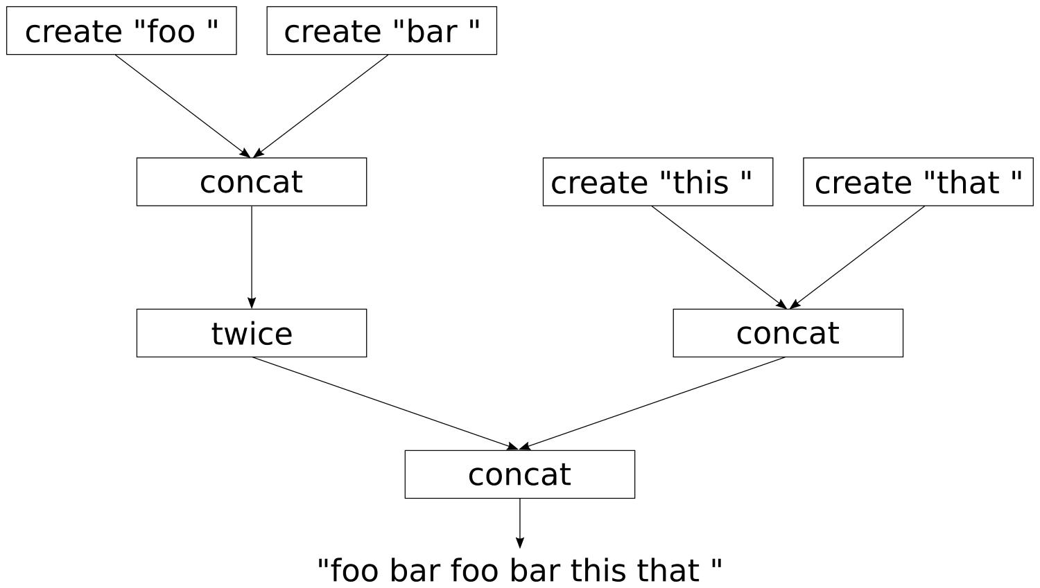
When implementing this in code, it is clear that everything can be implemented in a serial manner on one CPU core. Alternatively, all subtasks that depend on no other subtasks or other subtasks that already have been finished, can be executed concurrently on multiple CPU cores.
It might perhaps seem tedious to write such code, even with std::async because the dependencies between the subtasks need to be modeled. In this recipe, we will implement two little library helper functions that help to transform the normal functions create, concat, and twice to functions that work asynchronously. With those, we will find a really elegant way to set up the dependency graph. During execution, the graph will parallelize itself in a seemingly intelligent way in order to calculate the result as fast as possible.
In this section, we are going to implement some functions that simulate computation-intensive tasks that depend on each other, and let them run as parallel as possible:
#include <iostream>
#include <iomanip>
#include <thread>
#include <string>
#include <sstream>
#include <future>
using namespace std;
using namespace chrono_literals;
struct pcout : public stringstream {
static inline mutex cout_mutex;
~pcout() {
lock_guard<mutex> l {cout_mutex};
cout << rdbuf();
cout.flush();
}
};
static string create(const char *s)
{
pcout{} << "3s CREATE " << quoted(s) << 'n';
this_thread::sleep_for(3s);
return {s};
}
static string concat(const string &a, const string &b)
{
pcout{} << "5s CONCAT "
<< quoted(a) << " "
<< quoted(b) << 'n';
this_thread::sleep_for(5s);
return a + b;
}
static string twice(const string &s)
{
pcout{} << "3s TWICE " << quoted(s) << 'n';
this_thread::sleep_for(3s);
return s + s;
}
template <typename F>
static auto asynchronize(F f)
{
return [f](auto ... xs) {
return [=] () {
return async(launch::async, f, xs...);
};
};
}
template <typename F>
static auto fut_unwrap(F f)
{
return [f](auto ... xs) {
return f(xs.get()...);
};
}
template <typename F>
static auto async_adapter(F f)
{
return [f](auto ... xs) {
return [=] () {
return async(launch::async,
fut_unwrap(f), xs()...);
};
};
}
int main()
{
auto pcreate (asynchronize(create));
auto pconcat (async_adapter(concat));
auto ptwice (async_adapter(twice));
auto result (
pconcat(
ptwice(
pconcat(
pcreate("foo "),
pcreate("bar "))),
pconcat(
pcreate("this "),
pcreate("that "))));
cout << "Setup done. Nothing executed yet.n";
cout << result().get() << 'n';
}
$ ./chains
Setup done. Nothing executed yet.
3s CREATE "foo "
3s CREATE "bar "
3s CREATE "this "
3s CREATE "that "
5s CONCAT "this " "that "
5s CONCAT "foo " "bar "
3s TWICE "foo bar "
5s CONCAT "foo bar foo bar " "this that "
foo bar foo bar this that
A plain serial version of this program without any async and future magic would look like the following:
int main()
{
string result {
concat(
twice(
concat(
create("foo "),
create("bar "))),
concat(
create("this "),
create("that "))) };
cout << result << 'n';
}
In this recipe, we wrote the helper functions async_adapter and asynchronize that helped us create new functions from create, concat, and twice. We called those new asynchronous functions pcreate, pconcat, and ptwice.
Let us first ignore the complexity of the implementation of async_adapter and asynchronize, in order to first have a look what this got us.
The serial version looks similar to this code:
string result {concat( ... )};
cout << result << 'n';
The parallelized version looks similar to the following:
auto result (pconcat( ... ));
cout << result().get() << 'n';
Okay, now we get at the complicated part. The type of the parallelized result is not string, but a callable object that returns a future<string> on which we can call get(). This might indeed look crazy at first.
So, how and why did we exactly end up with callable objects that return futures? The problem with our create, concat, and twice methods is, that they are slow. (okay, we made them artificially slow, because we tried to model real life tasks that consume a lot of CPU time). But we identified that the dependency tree which describes the data flow has independent parts that could be executed in parallel. Let's have a look at two example schedules:
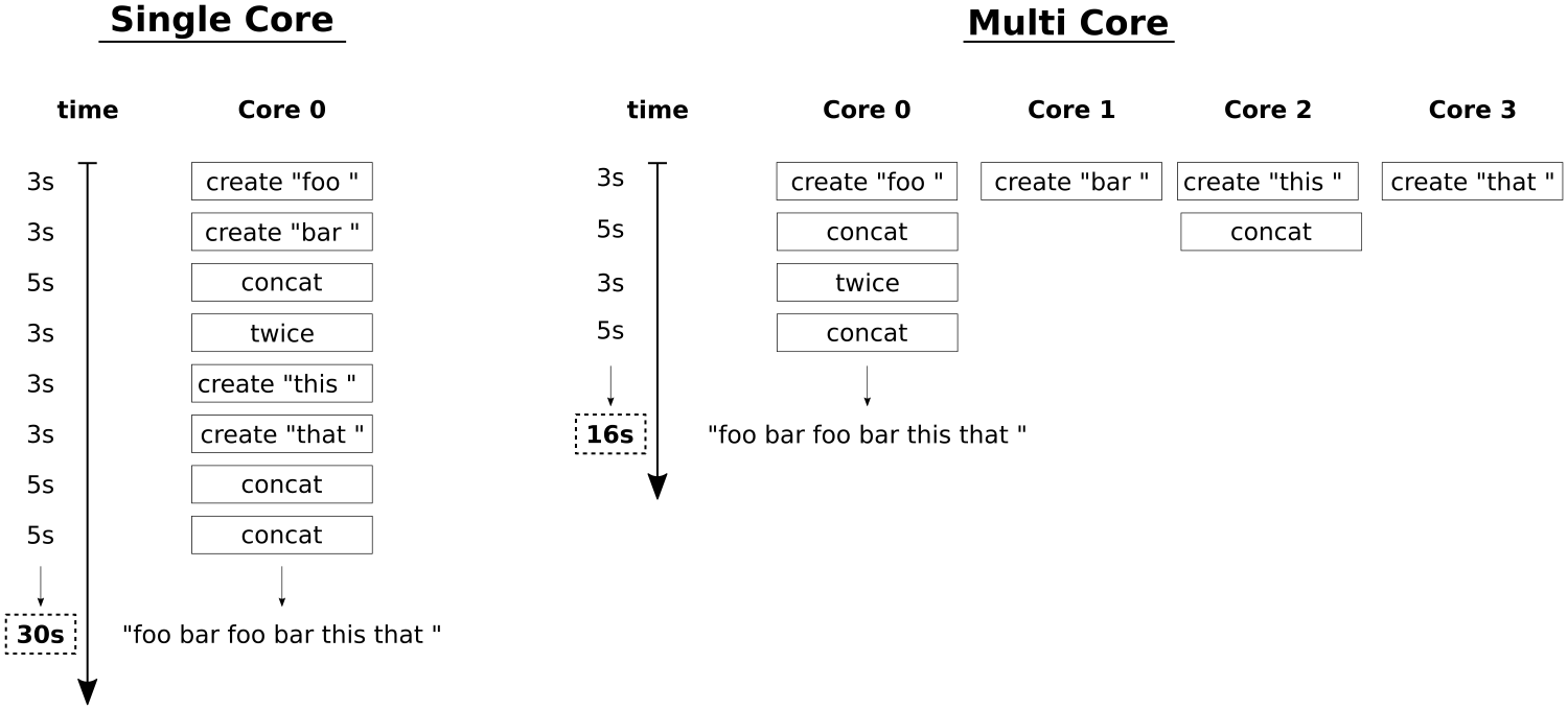
On the left side, we see a single core schedule. All the function calls have to be done one after each other because we have only a single CPU. That means, that when create costs 3 seconds, concat costs 5 seconds and twice costs 3 seconds, it will take 30 seconds to get the end result.
On the right side, we see a parallel schedule where as much is done in parallel as the dependencies between the function calls allow. In an ideal world with four cores, we can create all substrings at the same time, then concatenate them and so on. The minimal time to get the result with an optimal parallel schedule is 16 seconds. We cannot go faster if we cannot make the function calls themselves faster. With just four CPU cores we can achieve this execution time. We measurably achieved the optimal schedule. How did it work?
We could naively write the following code:
auto a (async(launch::async, create, "foo "));
auto b (async(launch::async, create, "bar "));
auto c (async(launch::async, create, "this "));
auto d (async(launch::async, create, "that "));
auto e (async(launch::async, concat, a.get(), b.get()));
auto f (async(launch::async, concat, c.get(), d.get()));
auto g (async(launch::async, twice, e.get()));
auto h (async(launch::async, concat, g.get(), f.get()));
This is a good start for a, b, c, and d, which represent the four substrings to begin with. These are created asynchronously in the background. Unfortunately, this code blocks on the line where we initialize e. In order to concatenate a and b, we need to call get() on both of them, which blocks until these values are ready. Obviously, this is not a good idea, because the parallelization stops being parallel on the first get() call. We need a better strategy.
Okay, so let us roll out the complicated helper functions we wrote. The first one is asynchronize:
template <typename F>
static auto asynchronize(F f)
{
return [f](auto ... xs) {
return [=] () {
return async(launch::async, f, xs...);
};
};
}
When we have a function int f(int, int) then we can do the following:
auto f2 ( asynchronize(f) );
auto f3 ( f2(1, 2) );
auto f4 ( f3() );
int result { f4.get() };
f2 is our asynchronous version of f. It can be called with the same arguments like f, because it mimics f. Then it returns a callable object, which we save in f3. f3 now captures f and the arguments 1, 2, but it did not call anything yet. This is just about the capturing.
When we call f3() now, then we finally get a future, because f3() does the async(launch::async, f, 1, 2); call! In that sense, the semantic meaning of f3 is "Take the captured function and the arguments, and throw them together into std::async.".
The inner lambda expression that does not accept any arguments gives us an indirection. With it, we can set up work for parallel dispatch but do not have to call anything that blocks, yet. We follow the same principle in the much more complicated function async_adapter:
template <typename F>
static auto async_adapter(F f)
{
return [f](auto ... xs) {
return [=] () {
return async(launch::async, fut_unwrap(f), xs()...);
};
};
}
This function does also first return a function that mimics f because it accepts the same arguments. Then that function returns a callable object that again accepts no arguments. And then that callable object finally differs from the other helper function.
What does the async(launch::async, fut_unwrap(f), xs()...); line mean? The xs()... part means, that all arguments that are saved in pack xs are assumed to be callable objects (like the ones we are creating all the time!), and so they are all called without arguments. Those callable objects that we are producing all the time themselves produce future values, on which we can call get(). This is where fut_unwrap comes into play:
template <typename F>
static auto fut_unwrap(F f)
{
return [f](auto ... xs) {
return f(xs.get()...);
};
}
fut_unwrap just transforms a function f into a function object that accepts a range of arguments. This function object does then call .get() on all of them and then finally forwards them to f.
Take your time to digest all of this. When we used this in our main function, then the auto result (pconcat(...)); call chain did just construct a large callable object that contains all functions and all arguments. No async call was done at this point yet. Then, when we called result(), we unleashed a little avalanche of async and .get() calls that come just in the right order to not block each other. In fact, no get() call happens before not all async calls have been dispatched.
In the end, we can finally call .get() on the future value that result() returned, and there we have our final string.
In this chapter, we will cover the following recipes:
Working with filesystem paths is always tedious if we don't have a library that helps us because there are many conditions that we need to handle.
Some paths are absolute, some are relative, and maybe they are not even straightforward because they also contain . (current directory) and .. (parent directory) indirections. Then, at the same time, different operating systems use the slash / to separate directories (Linux, MacOS, and different UNIX derivatives), or the backslash (Windows). And of course there are different types of files.
Since every other program that handles filesystem-related things needs such functionality, it is great to have the new filesystem library in the C++17 STL. The best thing about it is that it works the same way for different operating systems, so we don't have to write different code for versions of our programs that support different operating systems.
In this chapter, we will first see how the path class works, because it is most central to anything else in this library. Then, we will see how powerful but yet simple to use directory_iterator and recursive_directory_iterator classes are, while we do useful things with files. In the end, we will use some small and simple example tools that do some real-life tasks related to the filesystem. From this point, it will be easy to build more complex tools.
We start this chapter with a very simple example around the std::filesystem::path class and a helper function that intelligently normalizes filesystem paths.
The result of this recipe is a little application that takes any filesystem path and returns us the same path in normalized form. Normalized means that we get an absolute path that contains no . or .. path indirections.
While implementing that, we will also see what details we need to pay attention to when working with this basic part of the filesystem library.
In this section, we will implement a program that just accepts a filesystem path as a command-line argument and then prints it in normalized form.
#include <iostream>
#include <filesystem>
using namespace std;
using namespace filesystem;
int main(int argc, char *argv[])
{
if (argc != 2) {
cout << "Usage: " << argv[0] << " <path>n";
return 1;
}
const path dir {argv[1]};
if (!exists(dir)) {
cout << "Path " << dir << " does not exist.n";
return 1;
}
cout << canonical(dir).c_str() << 'n';
}
$ ./normalizer src
/Users/tfc/src
$ ./normalizer Desktop/../Documents/../src
/Users/tfc/src
As a starter on std::filesystem, this recipe is still fairly short and straightforward. We initialized a path object from a string that contains a filesystem path description. The std::filesystem::path class plays a very central role whenever we use the filesystem library because most of the functions and classes relate to it.
Using the filesystem::exists function, we were able to check if the path really exists. Up to that point, we could not be sure about that, because it is indeed possible to create path objects that do not relate to an existing filesystem object. exists just accepts a path instance and returns true if it really exists. The function is already able to determine itself if we gave it an absolute or a relative path, which makes it very comfortable to use.
Finally, we used filesystem::canonical on the directory in order to print it in normalized form.
path canonical(const path& p, const path& base = current_path());
canonical accepts a path and as an optional second argument, it accepts another path. The second path base is prepended to path p if p is a relative path. After doing that, canonical tries to remove any . and .. path indirections.
While printing, we used the .c_str() method on the canonicalized path. The reason for this is that the overload of operator<< for output streams surrounds paths with quotation marks, which we may not always want.
canonical throws a filesystem_error type exception if the path we want to canonicalize does not exist. In order to prevent that, we checked our filesystem path with exists. But was that check really sufficient to avoid getting unhandled exceptions? No.
Both exists and canonical can throw bad_alloc exceptions. If those hit us, one could argue that the program is doomed anyway. A far more critical, and also much more probable problem would occur if, between us checking if the file exists and canonicalizing it, someone else renames or deletes the underlying file! In that case, canonical would throw a filesystem_error, although we checked for the file's existence before.
Most filesystem functions have an additional overload that takes the same arguments, but also an std::error_code reference.
path canonical(const path& p, const path& base = current_path());
path canonical(const path& p, error_code& ec);
path canonical(const std::filesystem::path& p,
const std::filesystem::path& base,
std::error_code& ec );
This way we can choose if we surround our filesystem function calls with try-catch constructs or check the errors manually. Note that this only changes the behavior of filesystem-related errors! With and without the ec parameter, more fundamental exceptions, for example, bad_alloc, can still be thrown if the system runs out of memory.
In the last recipe, we already canonicalized/normalized paths. The filesystem::path class is, of course, capable of more things than just holding and checking paths. It also helps us in composing paths from strings easily, and also to decompose them again.
At this point, path does already abstract operating system details away from us, but there are also certain instances where we still need to keep such details in mind.
We will see how to deal with paths and their composition/decomposition by playing around with absolute and relative paths.
In this section, we will play around with absolute and relative paths in order to see the strengths of the path class and the helper functions around it.
#include <iostream>
#include <filesystem>
using namespace std;
using namespace filesystem;
int main()
{
path p {"testdir/foobar.txt"};
cout << "current_path : " << current_path()
<< "nabsolute_path : " << absolute(p)
<< "nsystem_complete : " << system_complete(p)
<< "ncanonical(p) : " << canonical(p)
<< 'n';
cout << path{"testdir"} / "foobar.txt" << 'n';
cout << "canonical testdir : "
<< canonical("foobar.txt",
current_path() / "testdir")
<< "ncanonical testdir 2 : "
<< canonical(p, current_path() / "testdir/..")
<< 'n';
cout << "equivalence: "
<< equivalent("testdir/foobar.txt",
"testdir/../testdir/foobar.txt")
<< 'n';
}
$ ./canonical_filepath
current_path : "/Users/tfc"
absolute_path : "/Users/tfc/testdir/foobar.txt"
system_complete : "/Users/tfc/testdir/foobar.txt"
canonical(p) : "/Users/tfc/testdir/foobar.txt"
"testdir/foobar.txt"
canonical testdir : "/Users/tfc/testdir/foobar.txt"
canonical testdir 2 : "/Users/tfc/testdir/foobar.txt"
equivalence: 1
$ ./canonial_filepath
current_path : "/Users/tfc"
absolute_path : "/Users/tfc/testdir/foobar.txt"
system_complete : "/Users/tfc/testdir/foobar.txt"
terminate called after throwing an instance of
'std::filesystem::v1::__cxx11::filesystem_error'
what(): filesystem error: cannot canonicalize:
No such file or directory [testdir/foobar.txt] [/Users/tfc]
The goal of this recipe is to see how easy it is to compose new paths on the fly. This is mainly because the path class has a handy overload for the / operator. In addition to that, the filesystem functions get along well with relative and absolute paths, as well as with paths that contain . and .. indirections.
There is quite a jungle of functions that return parts of a path instance, with or without transformations. We are not going to list all functions there are here because a short glance into the C++ reference is the best way to get an oversight.
The member functions of the path class, however, might be worth a closer look. Let's see which part of a path is returned by what member function of path. The following diagram also shows how Windows paths are slightly different from UNIX/Linux paths.
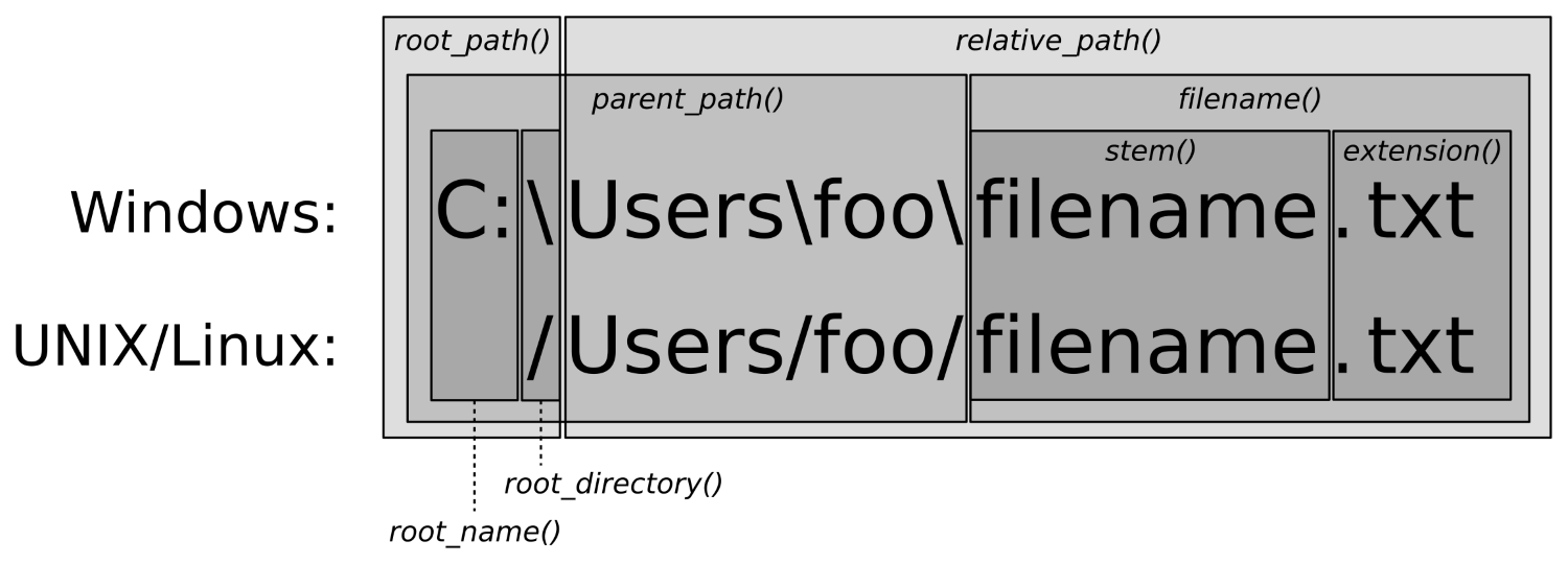
You can see that the diagram shows what the member functions of path return for an absolute path. For relative paths, root_path, root_name, and root_directory are empty. relative_path then just returns the path if it is relative already.
Of course, every operating system that offers filesystem support also comes with some kind of utility that does just list all files within a directory in the filesystem. The simplest examples are the ls command on Linux, MacOS, and other UNIX-related operating systems. In DOS and Windows, there is the dir command. Both list all files in a directory and provide supplemental information such as file size, permissions, and so on.
Reimplementing such a tool is, however, also a nice standard task to get going with directory and file traversal. So, let's just do that!
Our own ls/dir utility will be able to list all items in a directory by name, indicate what kind of items there are, list their access permission flags, and display the number of bytes they occupy on the filesystem.
In this section, we will implement a little tool that lists all files in any user provided directory. It will not only list the filenames, but also their type, size, and access permissions.
#include <iostream>
#include <sstream>
#include <iomanip>
#include <numeric>
#include <algorithm>
#include <vector>
#include <filesystem>
using namespace std;
using namespace filesystem;
static tuple<path, file_status, size_t>
file_info(const directory_entry &entry)
{
const auto fs (status(entry));
return {entry.path(),
fs,
is_regular_file(fs) ? file_size(entry.path()) : 0u};
}
static char type_char(file_status fs)
{
if (is_directory(fs)) { return 'd'; }
else if (is_symlink(fs)) { return 'l'; }
else if (is_character_file(fs)) { return 'c'; }
else if (is_block_file(fs)) { return 'b'; }
else if (is_fifo(fs)) { return 'p'; }
else if (is_socket(fs)) { return 's'; }
else if (is_other(fs)) { return 'o'; }
else if (is_regular_file(fs)) { return 'f'; }
return '?';
}
static string rwx(perms p)
{
auto check ([p](perms bit, char c) {
return (p & bit) == perms::none ? '-' : c;
});
return {check(perms::owner_read, 'r'),
check(perms::owner_write, 'w'),
check(perms::owner_exec, 'x'),
check(perms::group_read, 'r'),
check(perms::group_write, 'w'),
check(perms::group_exec, 'x'),
check(perms::others_read, 'r'),
check(perms::others_write, 'w'),
check(perms::others_exec, 'x')};
}
static string size_string(size_t size)
{
stringstream ss;
if (size >= 1000000000) {
ss << (size / 1000000000) << 'G';
} else if (size >= 1000000) {
ss << (size / 1000000) << 'M';
} else if (size >= 1000) {
ss << (size / 1000) << 'K';
} else { ss << size << 'B'; }
return ss.str();
}
int main(int argc, char *argv[])
{
path dir {argc > 1 ? argv[1] : "."};
if (!exists(dir)) {
cout << "Path " << dir << " does not exist.n";
return 1;
}
vector<tuple<path, file_status, size_t>> items;
transform(directory_iterator{dir}, {},
back_inserter(items), file_info);
for (const auto &[path, status, size] : items) {
cout << type_char(status)
<< rwx(status.permissions()) << " "
<< setw(4) << right << size_string(size)
<< " " << path.filename().c_str()
<< 'n';
}
}
$ ./list ~/Documents/cpp_reference/en/cpp
drwxrwxr-x 0B algorithm
frw-r--r-- 88K algorithm.html
drwxrwxr-x 0B atomic
frw-r--r-- 35K atomic.html
drwxrwxr-x 0B chrono
frw-r--r-- 34K chrono.html
frw-r--r-- 21K comment.html
frw-r--r-- 21K comments.html
frw-r--r-- 220K compiler_support.html
drwxrwxr-x 0B concept
frw-r--r-- 67K concept.html
drwxr-xr-x 0B container
frw-r--r-- 285K container.html
drwxrwxr-x 0B error
frw-r--r-- 52K error.html
In this recipe, we iterated over files, and for every file, we checked its status and size. While all our per-file operations are fairly straightforward and simple, our actual directory traversal looked a bit magic.
In order to traverse our directory, we just instantiated a directory_iterator and then iterated over it. Traversing a directory is fantastically simple with the filesystem library.
for (const directory_entry &e : directory_iterator{dir}) {
// do something
}
There is not much more to say about this class apart from the following things:
However, it might be noticeable that directory_iterator seems to be an iterator, and an iterable range at the same time. Why? In the minimal for loop example we just had a look at, it was used as an iterable range. In the actual recipe code, we used it like an iterator:
transform(directory_iterator{dir}, {},
back_inserter(items), file_info);
The truth is, it is just an iterator class type, but the std::begin and std::end functions provide overloads for this type. This way we can call the begin and end function on this kind of iterator and they return us iterators again. That might look strange at first sight, but it makes this class more useful.
Most operating systems come equipped with some kind of local search engine. Users can fire it up with some keyboard shortcut and then just enter what local file they are looking for.
Before such features came up, command-line users already searched through files with tools such as grep or awk. The user can simply type "grep -r foobar ." and the tool will crawl recursively through the current directory and find any file that contains the "foobar" string.
In this recipe, we will implement exactly such an application. Our little grep clone will just accept a pattern from the command line, and then recursively search through the directory we are in at the time of the application start. It will then print the name of every file that matches our pattern. The pattern matching will be applied linewise, so we can also print on which exact line numbers a file is matching the pattern.
We will implement a little tool that searches for user-provided text patterns in files. The tool works similar to the UNIX tool grep, but will not be as mature and powerful, for the sake of simplicity.
#include <iostream>
#include <fstream>
#include <regex>
#include <vector>
#include <string>
#include <filesystem>
using namespace std;
using namespace filesystem;
static vector<pair<size_t, string>>
matches(const path &p, const regex &re)
{
vector<pair<size_t, string>> d;
ifstream is {p.c_str()};
string s;
for (size_t line {1}; getline(is, s); ++line) {
if (regex_search(begin(s), end(s), re)) {
d.emplace_back(line, move(s));
}
}
return d;
}
int main(int argc, char *argv[])
{
if (argc != 2) {
cout << "Usage: " << argv[0] << " <pattern>n";
return 1;
}
regex pattern;
try { pattern = regex{argv[1]}; }
catch (const regex_error &e) {
cout << "Invalid regular expression provided.n";
return 1;
}
for (const auto &entry :
recursive_directory_iterator{current_path()}) {
auto ms (matches(entry.path(), pattern));
for (const auto &[number, content] : ms) {
cout << entry.path().c_str() << ":" << number
<< " - " << content << 'n';
}
}
}
foo
bar
baz
$ ./grepper bar
/Users/tfc/testdir/dir1/text1.txt:1 - foo bar bla blubb
/Users/tfc/testdir/foobar.txt:2 - bar
$ ./grepper baz
/Users/tfc/testdir/foobar.txt:3 - baz
Setting up and using a regular expression in order to filter the content of files is certainly the main task of this recipe. However, let's concentrate on recursive_directory_iterator because filtering recursively iterated files was just our motivation to use this special iterator class in this recipe.
Just like directory_iterator, recursive_directory_iterator iterates over elements of a directory. Its specialty is to do this recursively, as its name tells. Whenever it hits a filesystem element that is a directory, it will yield a directory_entry instance to this path, but then also descend down into it in order to iterate its children, too.
recursive_directory_iterator has some interesting member functions:
Another thing to know about is the directory_options enum class. The constructor of recursive_directory_iterator does indeed accept a value of this type as a second argument. The default value which we have been implicitly using is directory_options::none. The other values are:
These options can be combined with the | operator.
This recipe is motivated by a situation I find myself in pretty often. When collecting picture files from holidays, for example, from different friends and also different photo devices in one folder, the file endings often look different. Some JPEG files have a .jpg extension, some have .jpeg, and some others even have .JPEG.
Some people might prefer to homogenize all extensions. It would be useful to rename all files with a single command. At the same time, we could remove spaces ' ' and substitute them by underscores '_', for example.
In this recipe, we will implement such a tool and call it renamer. It will accept a range of input patterns and their substitutes like this:
$ renamer jpeg jpg JPEG jpg
In that case, renamer will iterate recursively through the current directory and search for the patterns jpeg and JPEG in all filenames. It will substitute both with jpg.
We will implement a tool that recursively scans all files within a directory and matches their filenames with patterns. All matches are replaced with user provided tokens and the affected files are renamed accordingly.
#include <iostream>
#include <regex>
#include <vector>
#include <filesystem>
using namespace std;
using namespace filesystem;
template <typename T>
static string replace(string s, const T &replacements)
{
for (const auto &[pattern, repl] : replacements) {
s = regex_replace(s, pattern, repl);
}
return s;
}
int main(int argc, char *argv[])
{
if (argc < 3 || argc % 2 != 1) {
cout << "Usage: " << argv[0]
<< " <pattern> <replacement> ...n";
return 1;
}
vector<pair<regex, string>> patterns;
for (int i {1}; i < argc; i += 2) {
patterns.emplace_back(argv[i], argv[i + 1]);
}
for (const auto &entry :
recursive_directory_iterator{current_path()}) {
path opath {entry.path()};
string rname {replace(opath.filename().string(),
patterns)};
path rpath {opath};
rpath.replace_filename(rname);
if (opath != rpath) {
cout << opath.c_str() << " --> "
<< rpath.filename().c_str() << 'n';
if (exists(rpath)) {
cout << "Error: Can't rename."
" Destination file exists.n";
} else {
rename(opath, rpath);
}
}
}
}
$ ls
birthday_party.jpeg holiday_in_dubai.jpg holiday_in_spain.jpg
trip_to_new_york.JPEG
$ ../renamer jpeg jpg JPEG jpg
/Users/tfc/pictures/birthday_party.jpeg --> birthday_party.jpg
/Users/tfc/pictures/trip_to_new_york.JPEG --> trip_to_new_york.jpg
$ ls
birthday_party.jpg holiday_in_dubai.jpg holiday_in_spain.jpg
trip_to_new_york.jpg
We already implemented a tool that works like ls on Linux/MacOS, or dir on Windows, but just as these tools, it doesn't print the file size for directories.
In order to get the size equivalent of a directory, we would have to descend down into it and sum up the size of all files that it contains.
In this recipe, we will implement a tool that does just that. The tool can be run on any folder and will summarize the accumulated size of all directory entries.
In this section, we will implement an app that iterates over a directory and lists the file size of each entry. This is simple for regular files, but if we are looking at a directory entry that itself is a directory, then we have to look into it and summarize the size of all the files it holds.
#include <iostream>
#include <sstream>
#include <iomanip>
#include <numeric>
#include <filesystem>
using namespace std;
using namespace filesystem;
static size_t entry_size(const directory_entry &entry)
{
if (!is_directory(entry)) { return file_size(entry); }
return accumulate(directory_iterator{entry}, {}, 0u,
[](size_t accum, const directory_entry &e) {
return accum + entry_size(e);
});
}
static string size_string(size_t size)
{
stringstream ss;
if (size >= 1000000000) {
ss << (size / 1000000000) << 'G';
} else if (size >= 1000000) {
ss << (size / 1000000) << 'M';
} else if (size >= 1000) {
ss << (size / 1000) << 'K';
} else { ss << size << 'B'; }
return ss.str();
}
int main(int argc, char *argv[])
{
path dir {argc > 1 ? argv[1] : "."};
if (!exists(dir)) {
cout << "Path " << dir << " does not exist.n";
return 1;
}
for (const auto &entry : directory_iterator{dir}) {
cout << setw(5) << right
<< size_string(entry_size(entry))
<< " " << entry.path().filename().c_str()
<< 'n';
}
}
$ ./file_size ~/Documents/cpp_reference/en/
19M c
12K c.html
147M cpp
17K cpp.html
22K index.html
22K Main_Page.html
The whole program revolves around using file_size on regular files. If the program sees a directory, it recursively descends down into it and calls file_size on all its entries.
The only thing we did to distinguish if we call file_size directly or if we need the recursion strategy was asking the is_directory predicate. This works well for directories that only contain regular files and directories.
As simple as our example program is, it would crash under the following conditions, because of unhandled exceptions:
In order to make this example recipe program more mature, we need more defensive programming against the wrong type of files and handling of exceptions.
In the last recipe, we implemented a tool that lists the size of all members of any directory.
In this recipe, we will be counting sizes recursively, too, but this time we will accumulate the size of each file to their filename extension. This way we can print the user a table that lists how many files of each file type we have, and what the average size of such file types is.
In this section, we will implement a little tool that recursively iterates over a given directory. While doing that, it counts the number and size of all files, grouped by their extensions. Finally, it prints which filename extensions exist within that directory, how many there are per extension, and their average file size.
#include <iostream>
#include <sstream>
#include <iomanip>
#include <map>
#include <filesystem>
using namespace std;
using namespace filesystem;
static string size_string(size_t size)
{
stringstream ss;
if (size >= 1000000000) {
ss << (size / 1000000000) << 'G';
} else if (size >= 1000000) {
ss << (size / 1000000) << 'M';
} else if (size >= 1000) {
ss << (size / 1000) << 'K';
} else { ss << size << 'B'; }
return ss.str();
}
static map<string, pair<size_t, size_t>> ext_stats(const path &dir)
{
map<string, pair<size_t, size_t>> m;
for (const auto &entry :
recursive_directory_iterator{dir}) {
const path p {entry.path()};
const file_status fs {status(p)};
if (is_directory(fs)) { continue; }
const string ext {p.extension().string()};
if (ext.length() == 0) { continue; }
const size_t size {file_size(p)};
auto &[size_accum, count] = m[ext];
size_accum += size;
count += 1;
}
return m;
}
int main(int argc, char *argv[])
{
path dir {argc > 1 ? argv[1] : "."};
if (!exists(dir)) {
cout << "Path " << dir << " does not exist.n";
return 1;
}
for (const auto &[ext, stats] : ext_stats(dir)) {
const auto &[accum_size, count] = stats;
cout << setw(15) << left << ext << ": "
<< setw(4) << right << count
<< " items, avg size "
<< setw(4) << size_string(accum_size / count)
<< 'n';
}
}
$ ./file_type ~/Documents/cpp_reference/
.css : 2 items, avg size 41K
.gif : 7 items, avg size 902B
.html : 4355 items, avg size 38K
.js : 3 items, avg size 4K
.php : 1 items, avg size 739B
.png : 34 items, avg size 2K
.svg : 53 items, avg size 6K
.ttf : 2 items, avg size 421K
There are a lot of tools that compress data in various ways. The most famous examples for file packing algorithms/formats are ZIP and RAR. Such tools try to reduce the size of files by reducing internal redundancy.
Before compressing files in archives, a very simple way to reduce disk usage is just deleting duplicate files. In this recipe, we will implement a little tool that crawls a directory recursively. While crawling, it will look for files that have the same content. If it finds such files, it will remove all duplicates but one. All removed files will be substituted with symbolic links that point to the now unique file. This saves spaces without any compression, while at the same time preserving all data.
In this section, we will implement a little tool that finds out which files in a directory are duplicates of each other. With that knowledge, it will remove all but one of all duplicated files, and substitute them with symbolic links, which reduces the folder size.
#include <iostream>
#include <fstream>
#include <unordered_map>
#include <filesystem>
using namespace std;
using namespace filesystem;
static size_t hash_from_path(const path &p)
{
ifstream is {p.c_str(),
ios::in | ios::binary};
if (!is) { throw errno; }
string s;
is.seekg(0, ios::end);
s.reserve(is.tellg());
is.seekg(0, ios::beg);
s.assign(istreambuf_iterator<char>{is}, {});
return hash<string>{}(s);
}
static size_t reduce_dupes(const path &dir)
{
unordered_map<size_t, path> m;
size_t count {0};
for (const auto &entry :
recursive_directory_iterator{dir}) {
const path p {entry.path()};
if (is_directory(p)) { continue; }
const auto &[it, success] =
m.try_emplace(hash_from_path(p), p);
if (!success) {
cout << "Removed " << p.c_str()
<< " because it is a duplicate of "
<< it->second.c_str() << 'n';
remove(p);
create_symlink(absolute(it->second), p);
++count;
}
}
return count;
}
int main(int argc, char *argv[])
{
if (argc != 2) {
cout << "Usage: " << argv[0] << " <path>n";
return 1;
}
path dir {argv[1]};
if (!exists(dir)) {
cout << "Path " << dir << " does not exist.n";
return 1;
}
const size_t dupes {reduce_dupes(dir)};
cout << "Removed " << dupes << " duplicates.n";
}
$ du -sh dupe_dir
1.1M dupe_dir
$ ./dupe_compress dupe_dir
Removed dupe_dir/dir2/bar.jpg because it is a duplicate of
dupe_dir/dir1/bar.jpg
Removed dupe_dir/dir2/base10.png because it is a duplicate of
dupe_dir/dir1/base10.png
Removed dupe_dir/dir2/baz.jpeg because it is a duplicate of
dupe_dir/dir1/baz.jpeg
Removed dupe_dir/dir2/feed_fish.jpg because it is a duplicate of
dupe_dir/dir1/feed_fish.jpg
Removed dupe_dir/dir2/foo.jpg because it is a duplicate of
dupe_dir/dir1/foo.jpg
Removed dupe_dir/dir2/fox.jpg because it is a duplicate of
dupe_dir/dir1/fox.jpg
Removed 6 duplicates.
$ du -sh dupe_dir
584K dupe_dir
We used the create_symlink function in order to make a filesystem entry point to another file in the filesystem. This way we can avoid having duplicate files. We could also have set a hard link using create_hard_link. Semantically, this is similar, but hard links have other technical implications than soft links. Different filesystem formats might not support hard links at all, or only a certain number of hard links that refer to the same file. Another problem is that hard links cannot link from one filesystem to the other.
However, apart from implementation details, there is one blatant error source when using create_symlink or create_hard_link. The following lines contain a bug. Can you spot it immediately?
path a {"some_dir/some_file.txt"};
path b {"other_dir/other_file.txt"};
remove(b);
create_symlink(a, b);
Nothing bad happens when executing this program, but the symlink will be broken. The symlink points to "some_dir/some_file.txt", which is wrong. The problem is that it should really either point to "/absolute/path/some_dir/some_file.txt", or "../some_dir/some_file.txt". The create_symlink call uses a correct absolute path if we write it as follows:
create_symlink(absolute(a), b);
We already noticed that our hash function is a too simple one. For the sake of keeping this recipe simple and without external dependencies, we chose this way.
What is the problem with our hash function? There are actually two problems:
If we are looking for a better hash function, we should take one that is fast, memory-friendly, and that makes sure that no two really large but different files get the same hash. The latter requirement is maybe the most important one. If we decide that one file is a duplicate of the other although they do not contain the same data, we surely have some data loss after deleting it.
Better hash algorithms are, for example, MD5 or one of the SHA variants. In order to get access to such functions in our program, we could use the OpenSSL cryptography API, for example.
This Learning Path combines some of the best that Packt has to offer in one complete, curated package. It includes content from the following Packt products:
Copyright © 2018 Packt Publishing
All rights reserved. No part of this learning path may be reproduced, stored in a retrieval system, or transmitted in any form or by any means, without the prior written permission of the publisher, except in the case of brief quotations embedded in critical articles or reviews.
Every effort has been made in the preparation of this learning path to ensure the accuracy of the information presented. However, the information contained in this learning path is sold without warranty, either express or implied. Neither the authors, nor Packt Publishing or its dealers and distributors, will be held liable for any damages caused or alleged to have been caused directly or indirectly by this learning path.
Packt Publishing has endeavored to provide trademark information about all of the companies and products mentioned in this learning path by the appropriate use of capitals. However, Packt Publishing cannot guarantee the accuracy of this information.
Authors: Jeganathan Swaminathan, Maya Posch, Jacek Galowicz
Reviewer: Brandon James, Louis E. Mauget, Arne Mertz
Content Development Editor: Priyanka Sawant
Graphics: Jisha Chirayal
Production Coordinator: Nilesh Mohite
Published on: April 2018
Production reference: 1060418
Published by Packt Publishing Ltd.
Livery Place
35 Livery Street
Birmingham
B3 2PB, UK.
ISBN 978-1-78883-139-0
Mapt is an online digital library that gives you full access to over 5,000 books and videos, as well as industry leading tools to help you plan your personal development and advance your career. For more information, please visit our website.
Spend less time learning and more time coding with practical eBooks and Videos from over 4,000 industry professionals
Improve your learning with Skill Plans built especially for you
Get a free eBook or video every month
Mapt is fully searchable
Copy and paste, print, and bookmark content
Did you know that Packt offers eBook versions of every book published, with PDF and ePub files available? You can upgrade to the eBook version at www.PacktPub.com and as a print book customer, you are entitled to a discount on the eBook copy. Get in touch with us at service@packtpub.com for more details.
At www.PacktPub.com, you can also read a collection of free technical articles, sign up for a range of free newsletters, and receive exclusive discounts and offers on Packt books and eBooks.
C++ has come a long way and has now been adopted in several contexts. Its key strengths are its software infrastructure and resource-constrained applications. The C++ 17 release will change the way developers write code, and this course will help you master your developing skills with C++. With real-world, practical examples explaining each concept, the course is divided into three modules where will begin by introducing you to the latest features in C++ 17. It encourages clean code practices in C++ in general and demonstrates the GUI app-development options in C++. You’ll get tips on avoiding memory leaks using smart-pointers.
In the next module, you’ll see how multi-threaded programming can help you achieve concurrency in your applications. We start with a brief introduction to the fundamentals of multithreading and concurrency concepts. We then take an in-depth look at how these concepts work at the hardware-level as well as how both operating systems and frameworks use these low-level functions.
You will learn about the native multithreading and concurrency support available in C++ since the 2011 revision, synchronization and communication between threads, debugging concurrent C++ applications, and the best programming practices in C++.
Moving on, you’ll get an in-depth understanding of the C++ Standard Template Library. Where we show implementation-specific, problem-solution approach that will help you quickly overcome hurdles. You will learn the core STL concepts, such as containers, algorithms, utility classes, lambda expressions, iterators, and more while working on practical real-world recipes. These recipes will help you get the most from the STL and show you how to program in a better way.
This course is for intermediate to advanced level C++ developers who want to get the most out of C++ to build concurrent and scalable application.
Section 1, Mastering C++ Programming, introducing you to the latest features in C++ 17 and STL. It encourages clean code practices in C++ in general and demonstrates the GUI app-development options in C++. You’ll get tips on avoiding memory leaks using smart-pointers.
Section 2, Mastering C++ Multithreading, you’ll see how multi-threaded programming can help you achieve concurrency in your applications. We start with a brief introduction to the fundamentals of multithreading and concurrency concepts. We then take an in-depth look at how these concepts work at the hardware-level as well as how both operating systems and frameworks use these low-level functions. You will learn about the native multithreading and concurrency support available in C++ since the 2011 revision, synchronization and communication between threads, debugging concurrent C++ applications, and the best programming practices in C++.
Section 3, C++17 STL Cookbook, you’ll get an in-depth understanding of the C++ Standard Template Library; we show implementation-specific, problem-solution approaches that will help you quickly overcome hurdles. You will learn the core STL concepts, such as containers, algorithms, utility classes, lambda expressions, iterators, and more while working on practical real-world recipes. These recipes will help you get the most from the STL and show you how to program in a better way.
A strong understanding of C++ language is highly recommended as the book is for the experienced developers. You will need any OS (Windows, Linux, or macOS) and any C++ compiler installed on your systems in order to get started.
You can download the example code files for this learning path from your account at www.packtpub.com. If you purchased this learning path elsewhere, you can visit www.packtpub.com/support and register to have the files emailed directly to you.
You can download the code files by following these steps:
Once the file is downloaded, please make sure that you unzip or extract the folder using the latest version of:
The code bundle for the learning path is also hosted on GitHub at https://github.com/PacktPublishing/Expert-Cpp-Programming. We also have other code bundles from our rich catalog of books and videos available at https://github.com/PacktPublishing/. Check them out!
There are a number of text conventions used throughout this book.
CodeInText: Indicates code words in text, database table names, folder names, filenames, file extensions, pathnames, dummy URLs, user input, and Twitter handles. Here is an example: "Mount the downloaded WebStorm-10*.dmg disk image file as another disk in your system."
A block of code is set as follows:
html, body, #map {
height: 100%;
margin: 0;
padding: 0
}
When we wish to draw your attention to a particular part of a code block, the relevant lines or items are set in bold:
[default]
exten => s,1,Dial(Zap/1|30)
exten => s,2,Voicemail(u100)
exten => s,102,Voicemail(b100)
exten => i,1,Voicemail(s0)
Any command-line input or output is written as follows:
$ mkdir css
$ cd css
Bold: Indicates a new term, an important word, or words that you see onscreen. For example, words in menus or dialog boxes appear in the text like this. Here is an example: "Select System info from the Administration panel."
Feedback from our readers is always welcome.
General feedback: Email feedback@packtpub.com and mention the learning path title in the subject of your message. If you have questions about any aspect of this learning path, please email us at questions@packtpub.com.
Errata: Although we have taken every care to ensure the accuracy of our content, mistakes do happen. If you have found a mistake in this learning path, we would be grateful if you would report this to us. Please visit www.packtpub.com/submit-errata, selecting your learning path, clicking on the Errata Submission Form link, and entering the details.
Piracy: If you come across any illegal copies of our works in any form on the Internet, we would be grateful if you would provide us with the location address or website name. Please contact us at copyright@packtpub.com with a link to the material.
If you are interested in becoming an author: If there is a topic that you have expertise in and you are interested in either writing or contributing to a book, please visit authors.packtpub.com.
Please leave a review. Once you have read and used this learning path, why not leave a review on the site that you purchased it from? Potential readers can then see and use your unbiased opinion to make purchase decisions, we at Packt can understand what you think about our products, and our authors can see your feedback on their book. Thank you!
For more information about Packt, please visit packtpub.com.
As you know, the C++ language is the brain child of Bjarne Stroustrup, who developed C++ in 1979. The C++ programming language is standardized by International Organization for Standardization (ISO). The initial standardization was published in 1998, commonly referred to as C++98, and the next standardization C++03 was published in 2003, which was primarily a bug fix release with just one language feature for value initialization. In August 2011, the C++11 standard was published with several additions to the core language, including several significant interesting changes to the Standard Template Library (STL); C++11 basically replaced the C++03 standard. C++14 was published in December, 2014 with some new features, and later, the C++17 standard was published on July 31, 2017. At the time of writing this book, C++17 is the latest revision of the ISO/IEC standard for the C++ programming language.
This chapter requires a compiler that supports C++17 features: gcc version 7 or later. As gcc version 7 is the latest version at the time of writing this book, I'll be using gcc version 7.1.0 in this chapter.
This chapter will cover the following topics:
Let's look into the STL topics one by one in the following sections.
The C++ Standard Template Library (STL) offers ready-made generic containers, algorithms that can be applied to the containers, and iterators to navigate the containers. The STL is implemented with C++ templates, and templates allow generic programming in C++.
The STL encourages a C++ developer to focus on the task at hand by freeing up the developer from writing low-level data structures and algorithms. The STL is a time-tested library that allows rapid application development.
The STL is an interesting piece of work and architecture. Its secret formula is compile-time polymorphism. To get better performance, the STL avoids dynamic polymorphism, saying goodbye to virtual functions. Broadly, the STL has the following four components:
The STL architecture stitches all the aforementioned four components together. It has many commonly used algorithms with performance guarantees. The interesting part about STL algorithms is that they work seamlessly without any knowledge about the containers that hold the data. This is made possible due to the iterators that offer high-level traversal APIs, which completely abstracts the underlying data structure used within a container. The STL makes use of operator overloading quite extensively. Let's understand the major components of STL one by one to get a good grasp of the STL conceptually.
The STL algorithms are powered by C++ templates; hence, the same algorithm works irrespective of what data type it deals with or independently of how the data is organized by a container. Interestingly, the STL algorithms are generic enough to support built-in and user-defined data types using templates. As a matter of fact, the algorithms interact with the containers via iterators. Hence, what matters to the algorithms is the iterator supported by the container. Having said that, the performance of an algorithm depends on the underlying data structure used within a container. Hence, certain algorithms work only on selective containers, as each algorithm supported by the STL expects a certain type of iterator.
An iterator is a design pattern, but interestingly, the STL work started much before
Gang of Four published their design patterns-related work to the software community. Iterators themselves are objects that allow traversing the containers to access, modify, and manipulate the data stored in the containers. Iterators do this so magically that we don't realize or need to know where and how the data is stored and retrieved.
The following image visually represents an iterator:
From the preceding image, you can understand that every iterator supports the begin() API, which returns the first element position, and the end() API returns one position past the last element in the container.
The STL broadly supports the following five types of iterators:
The container implements the iterator to let us easily retrieve and manipulate the data, without delving much into the technical details of a container.
The following table explains each of the five iterators:
|
The type of iterator |
Description |
|
Input iterator |
|
|
Output iterator |
|
|
Forward iterator |
|
|
Bidirectional iterator |
|
|
Random-access iterator |
|
STL containers are objects that typically grow and shrink dynamically. Containers use complex data structures to store the data under the hood and offer high-level functions to access the data without us delving into the complex internal implementation details of the data structure. STL containers are highly efficient and time-tested.
Every container uses different types of data structures to store, organize, and manipulate data in an efficient way. Though many containers may seem similar, they behave differently under the hood. Hence, the wrong choice of containers leads to application performance issues and unnecessary complexities.
Containers come in the following flavors:
The objects stored in the containers are copied or moved, and not referenced. We will explore every type of container in the upcoming sections with simple yet interesting examples.
Functors are objects that behave like regular functions. The beauty is that functors can be substituted in the place of function pointers. Functors are handy objects that let you extend or complement the behavior of an STL function without compromising the object-oriented coding principles.
Functors are easy to implement; all you need to do is overload the function operator. Functors are also referred to as functionoids.
The following code will demonstrate the way a simple functor can be implemented:
#include <iostream>
#include <vector>
#include <iterator>
#include <algorithm>
using namespace std;
template <typename T>
class Printer {
public:
void operator() ( const T& element ) {
cout << element << "t";
}
};
int main () {
vector<int> v = { 10, 20, 30, 40, 50 };
cout << "nPrint the vector entries using Functor" << endl;
for_each ( v.begin(), v.end(), Printer<int>() );
cout << endl;
return 0;
}
Let's quickly compile the program using the following command:
g++ main.cpp -std=c++17
./a.out
Let's check the output of the program:
Print the vector entries using Functor
10 20 30 40 50
We hope you realize how easy and cool a functor is.
The STL supports quite an interesting variety of sequence containers. Sequence containers store homogeneous data types in a linear fashion, which can be accessed sequentially. The STL supports the following sequence containers:
As the objects stored in an STL container are nothing but copies of the values, the STL expects certain basic requirements from the user-defined data types in order to hold those objects inside a container. Every object stored in an STL container must provide the following as a minimum requirement:
Let's explore the sequence containers one by one in the following subsections.
The STL array container is a fixed-size sequence container, just like a C/C++ built-in array, except that the STL array is size-aware and a bit smarter than the built-in C/C++ array. Let's understand an STL array with an example:
#include <iostream>
#include <array>
using namespace std;
int main () {
array<int,5> a = { 1, 5, 2, 4, 3 };
cout << "nSize of array is " << a.size() << endl;
auto pos = a.begin();
cout << endl;
while ( pos != a.end() )
cout << *pos++ << "t";
cout << endl;
return 0;
}
The preceding code can be compiled and the output can be viewed with the following commands:
g++ main.cpp -std=c++17
./a.out
The output of the program is as follows:
Size of array is 5
1 5 2 4 3
The following line declares an array of a fixed size (5) and initializes the array with five elements:
array<int,5> a = { 1, 5, 2, 4, 3 };
The size mentioned can't be changed once declared, just like a C/C++ built-in array. The array::size() method returns the size of the array, irrespective of how many integers are initialized in the initializer list. The auto pos = a.begin() method declares an iterator of array<int,5> and assigns the starting position of the array. The array::end() method points to one position after the last element in the array. The iterator behaves like or mimics a C++ pointer, and dereferencing the iterator returns the value pointed by the iterator. The iterator position can be moved forward and backwards with ++pos and --pos, respectively.
The following table shows some commonly used array APIs:
|
API |
Description |
|
at( int index ) |
This returns the value stored at the position referred to by the index. The index is a zero-based index. This API will throw an std::out_of_range exception if the index is outside the index range of the array. |
|
operator [ int index ] |
This is an unsafe method, as it won't throw any exception if the index falls outside the valid range of the array. This tends to be slightly faster than at, as this API doesn't perform bounds checking. |
|
front() |
This returns the first element in the array. |
|
back() |
This returns the last element in the array. |
|
begin() |
This returns the position of the first element in the array |
|
end() |
This returns one position past the last element in the array |
|
rbegin() |
This returns the reverse beginning position, that is, it returns the position of the last element in the array |
|
rend() |
This returns the reverse end position, that is, it returns one position before the first element in the array |
|
size() |
This returns the size of the array |
The array container supports random access; hence, given an index, the array container can fetch a value with a runtime complexity of O(1) or constant time.
The array container elements can be accessed in a reverse fashion using the reverse iterator:
#include <iostream>
#include <array>
using namespace std;
int main () {
array<int, 6> a;
int size = a.size();
for (int index=0; index < size; ++index)
a[index] = (index+1) * 100;
cout << "nPrint values in original order ..." << endl;
auto pos = a.begin();
while ( pos != a.end() )
cout << *pos++ << "t";
cout << endl;
cout << "nPrint values in reverse order ..." << endl;
auto rpos = a.rbegin();
while ( rpos != a.rend() )
cout << *rpos++ << "t";
cout << endl;
return 0;
}
We will use the following command to get the output:
./a.out
The output is as follows:
Print values in original order ...
100 200 300 400 500 600
Print values in reverse order ...
600 500 400 300 200 100
Vector is a quite useful sequence container, and it works exactly as an array, except that the vector can grow and shrink at runtime while an array is of a fixed size. However, the data structure used under the hood in an array and vector is a plain simple built-in C/C++ style array.
Let's look at the following example to understand vectors better:
#include <iostream>
#include <vector>
#include <algorithm>
using namespace std;
int main () {
vector<int> v = { 1, 5, 2, 4, 3 };
cout << "nSize of vector is " << v.size() << endl;
auto pos = v.begin();
cout << "nPrint vector elements before sorting" << endl;
while ( pos != v.end() )
cout << *pos++ << "t";
cout << endl;
sort( v.begin(), v.end() );
pos = v.begin();
cout << "nPrint vector elements after sorting" << endl;
while ( pos != v.end() )
cout << *pos++ << "t";
cout << endl;
return 0;
}
The preceding code can be compiled and the output can be viewed with the following commands:
g++ main.cpp -std=c++17
./a.out
The output of the program is as follows:
Size of vector is 5
Print vector elements before sorting
1 5 2 4 3
Print vector elements after sorting
1 2 3 4 5
The following line declares a vector and initializes the vector with five elements:
vector<int> v = { 1, 5, 2, 4, 3 };
However, a vector also allows appending values to the end of the vector by using the vector::push_back<data_type>( value ) API. The sort() algorithm takes two random access iterators that represent a range of data that must be sorted. As the vector internally uses a built-in C/C++ array, just like the STL array container, a vector also supports random access iterators; hence the sort() function is a highly efficient algorithm whose runtime complexity is logarithmic, that is, O(N log2 (N)).
The following table shows some commonly used vector APIs:
|
API |
Description |
|
at ( int index ) |
This returns the value stored at the indexed position. It throws the std::out_of_range exception if the index is invalid. |
|
operator [ int index ] |
This returns the value stored at the indexed position. It is faster than at( int index ), since no bounds checking is performed by this function. |
|
front() |
This returns the first value stored in the vector. |
|
back() |
This returns the last value stored in the vector. |
|
empty() |
This returns true if the vector is empty, and false otherwise. |
|
size() |
This returns the number of values stored in the vector. |
|
reserve( int size ) |
This reserves the initial size of the vector. When the vector size has reached its capacity, an attempt to insert new values requires vector resizing. This makes the insertion consume O(N) runtime complexity. The reserve() method is a workaround for the issue described. |
|
capacity() |
This returns the total capacity of the vector, while the size is the actual value stored in the vector. |
|
clear() |
This clears all the values. |
|
push_back<data_type>( value ) |
This adds a new value at the end of the vector. |
It would be really fun and convenient to read and print to/from the vector using istream_iterator and ostream_iterator. The following code demonstrates the use of a vector:
#include <iostream>
#include <vector>
#include <algorithm>
#include <iterator>
using namespace std;
int main () {
vector<int> v;
cout << "nType empty string to end the input once you are done feeding the vector" << endl;
cout << "nEnter some numbers to feed the vector ..." << endl;
istream_iterator<int> start_input(cin);
istream_iterator<int> end_input;
copy ( start_input, end_input, back_inserter( v ) );
cout << "nPrint the vector ..." << endl;
copy ( v.begin(), v.end(), ostream_iterator<int>(cout, "t") );
cout << endl;
return 0;
}
Basically, the copy algorithm accepts a range of iterators, where the first two arguments represent the source and the third argument represents the destination, which happens to be the vector:
istream_iterator<int> start_input(cin);
istream_iterator<int> end_input;
copy ( start_input, end_input, back_inserter( v ) );
The start_input iterator instance defines an istream_iterator iterator that receives input from istream and cin, and the end_input iterator instance defines an end-of-file delimiter, which is an empty string by default (""). Hence, the input can be terminated by typing "" in the command-line input terminal.
Similarly, let's understand the following code snippet:
cout << "nPrint the vector ..." << endl;
copy ( v.begin(), v.end(), ostream_iterator<int>(cout, "t") );
cout << endl;
The copy algorithm is used to copy the values from a vector, one element at a time, to ostream, separating the output with a tab character (t).
Every STL container has its own advantages and disadvantages. There is no single STL container that works better in all the scenarios. A vector internally uses an array data structure, and arrays are fixed in size in C/C++. Hence, when you attempt to add new values to the vector at the time the vector size has already reached its maximum capacity, then the vector will allocate new consecutive locations that can accommodate the old values and the new value in a contiguous location. It then starts copying the old values into the new locations. Once all the data elements are copied, the vector will invalidate the old location.
Whenever this happens, the vector insertion will take O(N) runtime complexity. As the size of the vector grows over time, on demand, the O(N) runtime complexity will show up a pretty bad performance. If you know the maximum size required, you could reserve so much initial size upfront in order to overcome this issue. However, not in all scenarios do you need to use a vector. Of course, a vector supports dynamic size and random access, which has performance benefits in some scenarios, but it is possible that the feature you are working on may not really need random access, in which case a list, deque, or some other container may work better for you.
The list STL container makes use of a doubly linked list data structure internally. Hence, a list supports only sequential access, and searching a random value in a list in the worst case may take O(N) runtime complexity. However, if you know for sure that you only need sequential access, the list does offer its own benefits. The list STL container lets you insert data elements at the end, in the front, or in the middle with a constant time complexity, that is, O(1) runtime complexity in the best, average, and worst case scenarios.
The following image demonstrates the internal data structure used by the list STL:
Let's write a simple program to get first-hand experience of using the list STL:
#include <iostream>
#include <list>
#include <iterator>
#include <algorithm>
using namespace std;
int main () {
list<int> l;
for (int count=0; count<5; ++count)
l.push_back( (count+1) * 100 );
auto pos = l.begin();
cout << "nPrint the list ..." << endl;
while ( pos != l.end() )
cout << *pos++ << "-->";
cout << " X" << endl;
return 0;
}
I'm sure that by now you have got a taste of the C++ STL, its elegance, and its power. Isn't it cool to observe that the syntax remains the same for all the STL containers? You may have observed that the syntax remains the same no matter whether you are using an array, a vector, or a list. Trust me, you will get the same impression when you explore the other STL containers as well.
Having said that, the previous code is self-explanatory, as we did pretty much the same with the other containers.
Let's try to sort the list, as shown in the following code:
#include <iostream>
#include <list>
#include <iterator>
#include <algorithm>
using namespace std;
int main () {
list<int> l = { 100, 20, 80, 50, 60, 5 };
auto pos = l.begin();
cout << "nPrint the list before sorting ..." << endl;
copy ( l.begin(), l.end(), ostream_iterator<int>( cout, "-->" ));
cout << "X" << endl;
l.sort();
cout << "nPrint the list after sorting ..." << endl;
copy ( l.begin(), l.end(), ostream_iterator<int>( cout, "-->" ));
cout << "X" << endl;
return 0;
}
Did you notice the sort() method? Yes, the list container has its own sorting algorithms. The reason for a list container to support its own version of a sorting algorithm is that the generic sort() algorithm expects a random access iterator, whereas a list container doesn't support random access. In such cases, the respective container will offer its own efficient algorithms to overcome the shortcoming.
Interestingly, the runtime complexity of the sort algorithm supported by a list is O (N log2 N).
The following table shows the most commonly used APIs of an STL list:
|
API |
Description |
|
front() |
This returns the first value stored in the list |
|
back() |
This returns the last value stored in the list |
|
size() |
This returns the count of values stored in the list |
|
empty() |
This returns true when the list is empty, and false otherwise |
|
clear() |
This clears all the values stored in the list |
|
push_back<data_type>( value ) |
This adds a value at the end of the list |
|
push_front<data_type>( value ) |
This adds a value at the front of the list |
|
merge( list ) |
This merges two sorted lists with values of the same type |
|
reverse() |
This reverses the list |
|
unique() |
This removes duplicate values from the list |
|
sort() |
This sorts the values stored in a list |
The STL's forward_list container is built on top of a singly linked list data structure; hence, it only supports navigation in the forward direction. As forward_list consumes one less pointer for every node in terms of memory and runtime, it is considered more efficient compared with the list container. However, as price for the extra edge of performance advantage, forward_list had to give up some functionalities.
The following diagram shows the internal data-structure used in forward_list:
Let's explore the following sample code:
#include <iostream>
#include <forward_list>
#include <iterator>
#include <algorithm>
using namespace std;
int main ( ) {
forward_list<int> l = { 10, 10, 20, 30, 45, 45, 50 };
cout << "nlist with all values ..." << endl;
copy ( l.begin(), l.end(), ostream_iterator<int>(cout, "t") );
cout << "nSize of list with duplicates is " << distance( l.begin(), l.end() ) << endl;
l.unique();
cout << "nSize of list without duplicates is " << distance( l.begin(), l.end() ) << endl;
l.resize( distance( l.begin(), l.end() ) );
cout << "nlist after removing duplicates ..." << endl;
copy ( l.begin(), l.end(), ostream_iterator<int>(cout, "t") );
cout << endl;
return 0;
}
The output can be viewed with the following command:
./a.out
The output will be as follows:
list with all values ...
10 10 20 30 45 45 50
Size of list with duplicates is 7
Size of list without duplicates is 5
list after removing duplicates ...
10 20 30 45 50
The following code declares and initializes the forward_list container with some unique values and some duplicate values:
forward_list<int> l = { 10, 10, 20, 30, 45, 45, 50 };
As the forward_list container doesn't support the size() function, we used the distance() function to find the size of the list:
cout << "nSize of list with duplicates is " << distance( l.begin(), l.end() ) << endl;
The following forward_list<int>::unique() function removes the duplicate integers and retains only the unique values:
l.unique();
The following table shows the commonly used forward_list APIs:
|
API |
Description |
|
front() |
This returns the first value stored in the forward_list container |
|
empty() |
This returns true when the forward_list container is empty and false, otherwise |
|
clear() |
This clears all the values stored in forward_list |
|
push_front<data_type>( value ) |
This adds a value to the front of forward_list |
|
merge( list ) |
This merges two sorted forward_list containers with values of the same type |
|
reverse() |
This reverses the forward_list container |
|
unique() |
This removes duplicate values from the forward_list container |
|
sort() |
This sorts the values stored in forward_list |
Let's explore one more example to get a firm understanding of the forward_list container:
#include <iostream>
#include <forward_list>
#include <iterator>
#include <algorithm>
using namespace std;
int main () {
forward_list<int> list1 = { 10, 20, 10, 45, 45, 50, 25 };
forward_list<int> list2 = { 20, 35, 27, 15, 100, 85, 12, 15 };
cout << "nFirst list before sorting ..." << endl;
copy ( list1.begin(), list1.end(), ostream_iterator<int>(cout, "t") );
cout << endl;
cout << "nSecond list before sorting ..." << endl;
copy ( list2.begin(), list2.end(), ostream_iterator<int>(cout, "t") );
cout << endl;
list1.sort();
list2.sort();
cout << "nFirst list after sorting ..." << endl;
copy ( list1.begin(), list1.end(), ostream_iterator<int>(cout, "t") );
cout << endl;
cout << "nSecond list after sorting ..." << endl;
copy ( list2.begin(), list2.end(), ostream_iterator<int>(cout, "t") );
cout << endl;
list1.merge ( list2 );
cout << "nMerged list ..." << endl;
copy ( list1.begin(), list1.end(), ostream_iterator<int>(cout, "t") );
cout << "nMerged list after removing duplicates ..." << endl;
list1.unique();
copy ( list1.begin(), list1.end(), ostream_iterator<int>(cout, "t") );
return 0;
}
The preceding code snippet is an interesting example that demonstrates the practical use of the sort(), merge(), and unique() STL algorithms.
The output can be viewed with the following command:
./a.out
The output of the program is as follows:
First list before sorting ...
10 20 10 45 45 50 25
Second list before sorting ...
20 35 27 15 100 85 12 15
First list after sorting ...
10 10 20 25 45 45 50
Second list after sorting ...
12 15 15 20 27 35 85 100
Merged list ...
10 10 12 15 15 20 20 25 27 35 45 45 50 85 100
Merged list after removing duplicates ...
10 12 15 20 25 27 35 45 50 85 100
The output and the program are pretty self-explanatory.
The deque container is a double-ended queue and the data structure used could be a dynamic array or a vector. In a deque, it is possible to insert an element both at the front and back, with a constant time complexity of O(1), unlike vectors, in which the time complexity of inserting an element at the back is O(1) while that for inserting an element at the front is O(N). The deque doesn't suffer from the problem of reallocation, which is suffered by a vector. However, all the benefits of a vector are there with deque, except that deque is slightly better in terms of performance as compared to a vector as there are several rows of dynamic arrays or vectors in each row.
The following diagram shows the internal data structure used in a deque container:
Let's write a simple program to try out the deque container:
#include <iostream>
#include <deque>
#include <algorithm>
#include <iterator>
using namespace std;
int main () {
deque<int> d = { 10, 20, 30, 40, 50 };
cout << "nInitial size of deque is " << d.size() << endl;
d.push_back( 60 );
d.push_front( 5 );
cout << "nSize of deque after push back and front is " << d.size() << endl;
copy ( d.begin(), d.end(), ostream_iterator<int>( cout, "t" ) );
d.clear();
cout << "nSize of deque after clearing all values is " << d.size() <<
endl;
cout << "nIs the deque empty after clearing values ? " << ( d.empty()
? "true" : "false" ) << endl;
return 0;
}
The output can be viewed with the following command:
./a.out
The output of the program is as follows:
Intitial size of deque is 5
Size of deque after push back and front is 7
Print the deque ...
5 10 20 30 40 50 60
Size of deque after clearing all values is 0
Is the deque empty after clearing values ? true
The following table shows the commonly used deque APIs:
|
API |
Description |
|
at ( int index ) |
This returns the value stored at the indexed position. It throws the std::out_of_range exception if the index is invalid. |
|
operator [ int index ] |
This returns the value stored at the indexed position. It is faster than at( int index ) since no bounds checking is performed by this function. |
|
front() |
This returns the first value stored in the deque. |
|
back() |
This returns the last value stored in the deque. |
|
empty() |
This returns true if the deque is empty and false, otherwise. |
|
size() |
This returns the number of values stored in the deque. |
|
capacity() |
This returns the total capacity of the deque, while size() returns the actual number of values stored in the deque. |
|
clear() |
This clears all the values. |
|
push_back<data_type>( value ) |
This adds a new value at the end of the deque. |
Associative containers store data in a sorted fashion, unlike the sequence containers. Hence, the order in which the data is inserted will not be retained by the associative containers. Associative containers are highly efficient in searching a value with O( log n ) runtime complexity. Every time a new value gets added to the container, the container will reorder the values stored internally if required.
The STL supports the following types of associative containers:
Associative containers organize the data as key-value pairs. The data will be sorted based on the key for random and faster access. Associative containers come in two flavors:
The following associative containers come under ordered containers, as they are ordered/sorted in a particular fashion. Ordered associative containers generally use some form of Binary Search Tree (BST); usually, a red-black tree is used to store the data:
The following associative containers come under unordered containers, as they are not ordered in any particular fashion and they use hash tables:
Let's understand the previously mentioned containers with examples in the following subsections.
A set container stores only unique values in a sorted fashion. A set organizes the values using the value as a key. The set container is immutable, that is, the values stored in a set can't be modified; however, the values can be deleted. A set generally uses a red-black tree data structure, which is a form of balanced BST. The time complexity of set operations are guaranteed to be O ( log N ).
Let's write a simple program using a set:
#include <iostream>
#include <set>
#include <vector>
#include <iterator>
#include <algorithm>
using namespace std;
int main( ) {
set<int> s1 = { 1, 3, 5, 7, 9 };
set<int> s2 = { 2, 3, 7, 8, 10 };
vector<int> v( s1.size() + s2.size() );
cout << "nFirst set values are ..." << endl;
copy ( s1.begin(), s1.end(), ostream_iterator<int> ( cout, "t" ) );
cout << endl;
cout << "nSecond set values are ..." << endl;
copy ( s2.begin(), s2.end(), ostream_iterator<int> ( cout, "t" ) );
cout << endl;
auto pos = set_difference ( s1.begin(), s1.end(), s2.begin(), s2.end(), v.begin() );
v.resize ( pos - v.begin() );
cout << "nValues present in set one but not in set two are ..." << endl;
copy ( v.begin(), v.end(), ostream_iterator<int> ( cout, "t" ) );
cout << endl;
v.clear();
v.resize ( s1.size() + s2.size() );
pos = set_union ( s1.begin(), s1.end(), s2.begin(), s2.end(), v.begin() );
v.resize ( pos - v.begin() );
cout << "nMerged set values in vector are ..." << endl;
copy ( v.begin(), v.end(), ostream_iterator<int> ( cout, "t" ) );
cout << endl;
return 0;
}
The output can be viewed with the following command:
./a.out
The output of the program is as follows:
First set values are ...
1 3 5 7 9
Second set values are ...
2 3 7 8 10
Values present in set one but not in set two are ...
1 5 9
Merged values of first and second set are ...
1 2 3 5 7 8 9 10
The following code declares and initializes two sets, s1 and s2:
set<int> s1 = { 1, 3, 5, 7, 9 };
set<int> s2 = { 2, 3, 7, 8, 10 };
The following line will ensure that the vector has enough room to store the values in the resultant vector:
vector<int> v( s1.size() + s2.size() );
The following code will print the values in s1 and s2:
cout << "nFirst set values are ..." << endl;
copy ( s1.begin(), s1.end(), ostream_iterator<int> ( cout, "t" ) );
cout << endl;
cout << "nSecond set values are ..." << endl;
copy ( s2.begin(), s2.end(), ostream_iterator<int> ( cout, "t" ) );
cout << endl;
The set_difference() algorithm will populate the vector v with values only present in set s1 but not in s2. The iterator, pos, will point to the last element in the vector; hence, the vector resize will ensure that the extra spaces in the vector are removed:
auto pos = set_difference ( s1.begin(), s1.end(), s2.begin(), s2.end(), v.begin() );
v.resize ( pos - v.begin() );
The following code will print the values populated in the vector v:
cout << "nValues present in set one but not in set two are ..." << endl;
copy ( v.begin(), v.end(), ostream_iterator<int> ( cout, "t" ) );
cout << endl;
The set_union() algorithm will merge the contents of sets s1 and s2 into the vector, and the vector is then resized to fit only the merged values:
pos = set_union ( s1.begin(), s1.end(), s2.begin(), s2.end(), v.begin() );
v.resize ( pos - v.begin() );
The following code will print the merged values populated in the vector v:
cout << "nMerged values of first and second set are ..." << endl;
copy ( v.begin(), v.end(), ostream_iterator<int> ( cout, "t" ) );
cout << endl;
The following table describes the commonly used set APIs:
|
API |
Description |
|
insert( value ) |
This inserts a value into the set |
|
clear() |
This clears all the values in the set |
|
size() |
This returns the total number of entries present in the set |
|
empty() |
This will print true if the set is empty, and returns false otherwise |
|
find() |
This finds the element with the specified key and returns the iterator position |
|
equal_range() |
This returns the range of elements matching a specific key |
|
lower_bound() |
This returns an iterator to the first element not less than the given key |
|
upper_bound() |
This returns an iterator to the first element greater than the given key |
A map stores the values organized by keys. Unlike a set, a map has a dedicated key per value. Maps generally use a red-black tree as an internal data structure, which is a balanced BST that guarantees O( log N ) runtime efficiency for searching or locating a value in the map. The values stored in a map are sorted based on the key, using a red-black tree. The keys used in a map must be unique. A map will not retain the sequences of the input as it reorganizes the values based on the key, that is, the red-black tree will be rotated to balance the red-black tree height.
Let's write a simple program to understand map usage:
#include <iostream>
#include <map>
#include <iterator>
#include <algorithm>
using namespace std;
int main ( ) {
map<string, long> contacts;
contacts["Jegan"] = 123456789;
contacts["Meena"] = 523456289;
contacts["Nitesh"] = 623856729;
contacts["Sriram"] = 993456789;
auto pos = contacts.find( "Sriram" );
if ( pos != contacts.end() )
cout << pos->second << endl;
return 0;
}
Let's compile and check the output of the program:
g++ main.cpp -std=c++17
./a.out
The output is as follows:
Mobile number of Sriram is 8901122334
The following line declares a map with a string name as the key and a long mobile number as the value stored in the map:
map< string, long > contacts;
The following code snippet adds four contacts organized by name as the key:
contacts[ "Jegan" ] = 1234567890;
contacts[ "Meena" ] = 5784433221;
contacts[ "Nitesh" ] = 4567891234;
contacts[ "Sriram" ] = 8901122334;
The following line will try to locate the contact with the name, Sriram, in the contacts map; if Sriram is found, then the find() function will return the iterator pointing to the location of the key-value pair; otherwise it returns the contacts.end() position:
auto pos = contacts.find( "Sriram" );
The following code verifies whether the iterator, pos, has reached contacts.end() and prints the contact number. Since the map is an associative container, it stores a key=>value pair; hence, pos->first indicates the key and pos->second indicates the value:
if ( pos != contacts.end() )
cout << "nMobile number of " << pos->first << " is " << pos->second << endl;
else
cout << "nContact not found." << endl;
The following table shows the commonly used map APIs:
|
API |
Description |
|
at ( key ) |
This returns the value for the corresponding key if the key is found; otherwise it throws the std::out_of_range exception |
|
operator[ key ] |
This updates an existing value for the corresponding key if the key is found; otherwise it will add a new entry with the respective key=>value supplied |
|
empty() |
This returns true if the map is empty, and false otherwise |
|
size() |
This returns the count of the key=>value pairs stored in the map |
|
clear() |
This clears the entries stored in the map |
|
count() |
This returns the number of elements matching the given key |
|
find() |
This finds the element with the specified key |
A multiset container works in a manner similar to a set container, except for the fact that a set allows only unique values to be stored whereas a multiset lets you store duplicate values. As you know, in the case of set and multiset containers, the values themselves are used as keys to organize the data. A multiset container is just like a set; it doesn't allow modifying the values stored in the multiset.
Let's write a simple program using a multiset:
#include <iostream>
#include <set>
#include <iterator>
#include <algorithm>
using namespace std;
int main() {
multiset<int> s = { 10, 30, 10, 50, 70, 90 };
cout << "nMultiset values are ..." << endl;
copy ( s.begin(), s.end(), ostream_iterator<int> ( cout, "t" ) );
cout << endl;
return 0;
}
The output can be viewed with the following command:
./a.out
The output of the program is as follows:
Multiset values are ...
10 30 10 50 70 90
Interestingly, in the preceding output, you can see that the multiset holds duplicate values.
A multimap works exactly as a map, except that a multimap container will allow multiple values to be stored with the same key.
Let's explore the multimap container with a simple example:
#include <iostream>
#include <map>
#include <vector>
#include <iterator>
#include <algorithm>
using namespace std;
int main() {
multimap< string, long > contacts = {
{ "Jegan", 2232342343 },
{ "Meena", 3243435343 },
{ "Nitesh", 6234324343 },
{ "Sriram", 8932443241 },
{ "Nitesh", 5534327346 }
};
auto pos = contacts.find ( "Nitesh" );
int count = contacts.count( "Nitesh" );
int index = 0;
while ( pos != contacts.end() ) {
cout << "\nMobile number of " << pos->first << " is " <<
pos->second << endl;
++index;
++pos;
if ( index == count )
break;
}
return 0;
}
The program can be compiled and the output can be viewed with the following commands:
g++ main.cpp -std=c++17
./a.out
The output of the program is as follows:
Mobile number of Nitesh is 6234324343
Mobile number of Nitesh is 5534327346
An unordered set works in a manner similar to a set, except that the internal behavior of these containers differs. A set makes use of red-black trees while an unordered set makes use of hash tables. The time complexity of set operations is O( log N) while the time complexity of unordered set operations is O(1); hence, the unordered set tends to be faster than the set.
The values stored in an unordered set are not organized in any particular fashion, unlike in a set, which stores values in a sorted fashion. If performance is the criteria, then an unordered set is a good bet; however, if iterating the values in a sorted fashion is a requirement, then set is a good choice.
An unordered map works in a manner similar to a map, except that the internal behavior of these containers differs. A map makes use of red-black trees while unordered map makes use of hash tables. The time complexity of map operations is O( log N) while that of unordered map operations is O(1); hence, an unordered map tends to be faster than a map.
The values stored in an unordered map are not organized in any particular fashion, unlike in a map where values are sorted by keys.
An unordered multiset works in a manner similar to a multiset, except that the internal behavior of these containers differs. A multiset makes use of red-black trees while an unordered multiset makes use of hash tables. The time complexity of multiset operations is O( log N) while that of unordered multiset operations is O(1). Hence, an unordered multiset tends to be faster than a multiset.
The values stored in an unordered multiset are not organized in any particular fashion, unlike in a multiset where values are stored in a sorted fashion. If performance is the criteria, unordered multisets are a good bet; however, if iterating the values in a sorted fashion is a requirement, then multiset is a good choice.
An unordered multimap works in a manner similar to a multimap, except that the internal behavior of these containers differs. A multimap makes use of red-black trees while an unordered multimap makes use of hash tables. The time complexity of multimap operations is O( log N) while that of unordered multimap operations is O(1); hence, an unordered multimap tends to be faster than a multimap.
The values stored in an unordered multimap are not organized in any particular fashion, unlike in multimaps where values are sorted by keys. If performance is the criteria, then an unordered multimap is a good bet; however, if iterating the values in a sorted fashion is a requirement, then multimap is a good choice.
Container adapters adapt existing containers to provide new containers. In simple terms, STL extension is done with composition instead of inheritance.
STL containers can't be extended by inheritance, as their constructors aren't virtual. Throughout the STL, you can observe that while static polymorphism is used both in terms of operator overloading and templates, dynamic polymorphism is consciously avoided for performance reasons. Hence, extending the STL by subclassing the existing containers isn't a good idea, as it would lead to memory leaks because container classes aren't designed to behave like base classes.
The STL supports the following container adapters:
Let's explore the container adapters in the following subsections.
Stack is not a new container; it is a template adapter class. The adapter containers wrap an existing container and provide high-level functionalities. The stack adapter container offers stack operations while hiding the unnecessary functionalities that are irrelevant for a stack. The STL stack makes use of a deque container by default; however, we can instruct the stack to use any existing container that meets the requirement of the stack during the stack instantiation.
Deques, lists, and vectors meet the requirements of a stack adapter.
A stack operates on the Last In First Out (LIFO) philosophy.
The following table shows commonly used stack APIs:
|
API |
Description |
|
top() |
This returns the top-most value in the stack, that is, the value that was added last |
|
push<data_type>( value ) |
This will push the value provided to the top of the stack |
|
pop() |
This will remove the top-most value from the stack |
|
size() |
This returns the number of values present in the stack |
|
empty() |
This returns true if the stack is empty; otherwise it returns false |
It's time to get our hands dirty; let's write a simple program to use a stack:
#include <iostream>
#include <stack>
#include <iterator>
#include <algorithm>
using namespace std;
int main ( ) {
stack<string> spoken_languages;
spoken_languages.push ( "French" );
spoken_languages.push ( "German" );
spoken_languages.push ( "English" );
spoken_languages.push ( "Hindi" );
spoken_languages.push ( "Sanskrit" );
spoken_languages.push ( "Tamil" );
cout << "nValues in Stack are ..." << endl;
while ( ! spoken_languages.empty() ) {
cout << spoken_languages.top() << endl;
spoken_languages.pop();
}
cout << endl;
return 0;
}
The program can be compiled and the output can be viewed with the following command:
g++ main.cpp -std=c++17
./a.out
The output of the program is as follows:
Values in Stack are ...
Tamil
Kannada
Telugu
Sanskrit
Hindi
English
German
French
From the preceding output, we can see the LIFO behavior of stack.
A queue works based on the First In First Out (FIFO) principle. A queue is not a new container; it is a templatized adapter class that wraps an existing container and provides the high-level functionalities that are required for queue operations, while hiding the unnecessary functionalities that are irrelevant for a queue. The STL queue makes use of a deque container by default; however, we can instruct the queue to use any existing container that meets the requirement of the queue during the queue instantiation.
In a queue, new values can be added at the back and removed from the front. Deques, lists, and vectors meet the requirements of a queue adapter.
The following table shows the commonly used queue APIs:
|
API |
Description |
|
push() |
This appends a new value at the back of the queue |
|
pop() |
This removes the value at the front of the queue |
|
front() |
This returns the value in the front of the queue |
|
back() |
This returns the value at the back of the queue |
|
empty() |
This returns true when the queue is empty; otherwise it returns false |
|
size() |
This returns the number of values stored in the queue |
Let's use a queue in the following program:
#include <iostream>
#include <queue>
#include <iterator>
#include <algorithm>
using namespace std;
int main () {
queue<int> q;
q.push ( 100 );
q.push ( 200 );
q.push ( 300 );
cout << "nValues in Queue are ..." << endl;
while ( ! q.empty() ) {
cout << q.front() << endl;
q.pop();
}
return 0;
}
The program can be compiled and the output can be viewed with the following commands:
g++ main.cpp -std=c++17
./a.out
The output of the program is as follows:
Values in Queue are ...
100
200
300
From the preceding output, you can observe that the values were popped out in the same sequence that they were pushed in, that is, FIFO.
A priority queue is not a new container; it is a templatized adapter class that wraps an existing container and provides high-level functionalities that are required for priority queue operations, while hiding the unnecessary functionalities that are irrelevant for a priority queue. A priority queue makes use of a vector container by default; however, a deque container also meets the requirement of the priority queue. Hence, during the priority queue instantiation, you could instruct the priority queue to make use of a deque as well.
A priority queue organizes the data in such a way that the highest priority value appears first; in other words, the values are sorted in a descending order.
The deque and vector meet the requirements of a priority queue adaptor.
The following table shows commonly used priority queue APIs:
|
API |
Description |
|
push() |
This appends a new value at the back of the priority queue |
|
pop() |
This removes the value at the front of the priority queue |
|
empty() |
This returns true when the priority queue is empty; otherwise it returns false |
|
size() |
This returns the number of values stored in the priority queue |
|
top() |
This returns the value in the front of the priority queue |
Let's write a simple program to understand priority_queue:
#include <iostream>
#include <queue>
#include <iterator>
#include <algorithm>
using namespace std;
int main () {
priority_queue<int> q;
q.push( 100 );
q.push( 50 );
q.push( 1000 );
q.push( 800 );
q.push( 300 );
cout << "nSequence in which value are inserted are ..." << endl;
cout << "100t50t1000t800t300" << endl;
cout << "Priority queue values are ..." << endl;
while ( ! q.empty() ) {
cout << q.top() << "t";
q.pop();
}
cout << endl;
return 0;
}
The program can be compiled and the output can be viewed with the following command:
g++ main.cpp -std=c++17
./a.out
The output of the program is as follows:
Sequence in which value are inserted are ...
100 50 1000 800 300
Priority queue values are ...
1000 800 300 100 50
From the preceding output, you can observe that priority_queue is a special type of queue that reorders the inputs in such a way that the highest value appears first.
In this chapter you learned about ready-made generic containers, functors, iterators, and algorithms. You also learned set, map, multiset, and multimap associative containers, their internal data structures, and common algorithms that can be applied on them. Further you learned how to use the various containers with practical hands-on code samples.
In the next chapter, you will learn template programming, which helps you master the essentials of templates.
In this chapter, we will cover the following topics:
Let's now start learning generic programming.
Generic programming is a style of programming that helps you develop reusable code or generic algorithms that can be applied to a wide variety of data types. Whenever a generic algorithm is invoked, the data types will be supplied as parameters with a special syntax.
Let's say we would like to write a sort() function, which takes an array of inputs that needs to be sorted in an ascending order. Secondly, we need the sort() function to sort int, double, char, and string data types. There are a couple of ways this can be solved:
Well, both approaches have their own merits and demerits. The advantage of the first approach is that, since there are dedicated functions for the int, double, char, and string data types, the compiler will be able to perform type checking if an incorrect data type is supplied. The disadvantage of the first approach is that we have to write four different functions even though the logic remains the same across all the functions. If a bug is identified in the algorithm, it must be fixed separately in all four functions; hence, heavy maintenance efforts are required. If we need to support another data type, we will end up writing one more function, and this will keep growing as we need to support more data types.
The advantage of the second approach is that we could just write one macro for all the data types. However, one very discouraging disadvantage is that the compiler will not be able to perform type checking, and this approach is more prone to errors and may invite many unexpected troubles. This approach is dead against object-oriented coding principles.
C++ supports generic programming with templates, which has the following benefits:
However, the disadvantages are as follows:
A function template lets you parameterize a data type. The reason this is referred to as generic programming is that a single template function will support many built-in and user-defined data types. A templatized function works like a C-style macro, except for the fact that the C++ compiler will type check the function when we supply an incompatible data type at the time of invoking the template function.
It will be easier to understand the template concept with a simple example, as follows:
#include <iostream>
#include <algorithm>
#include <iterator>
using namespace std;
template <typename T, int size>
void sort ( T input[] ) {
for ( int i=0; i<size; ++i) {
for (int j=0; j<size; ++j) {
if ( input[i] < input[j] )
swap (input[i], input[j] );
}
}
}
int main () {
int a[10] = { 100, 10, 40, 20, 60, 80, 5, 50, 30, 25 };
cout << "nValues in the int array before sorting ..." << endl;
copy ( a, a+10, ostream_iterator<int>( cout, "t" ) );
cout << endl;
::sort<int, 10>( a );
cout << "nValues in the int array after sorting ..." << endl;
copy ( a, a+10, ostream_iterator<int>( cout, "t" ) );
cout << endl;
double b[5] = { 85.6d, 76.13d, 0.012d, 1.57d, 2.56d };
cout << "nValues in the double array before sorting ..." << endl;
copy ( b, b+5, ostream_iterator<double>( cout, "t" ) );
cout << endl;
::sort<double, 5>( b );
cout << "nValues in the double array after sorting ..." << endl;
copy ( b, b+5, ostream_iterator<double>( cout, "t" ) );
cout << endl;
string names[6] = {
"Rishi Kumar Sahay",
"Arun KR",
"Arun CR",
"Ninad",
"Pankaj",
"Nikita"
};
cout << "nNames before sorting ..." << endl;
copy ( names, names+6, ostream_iterator<string>( cout, "n" ) );
cout << endl;
::sort<string, 6>( names );
cout << "nNames after sorting ..." << endl;
copy ( names, names+6, ostream_iterator<string>( cout, "n" ) );
cout << endl;
return 0;
}
Run the following commands:
g++ main.cpp -std=c++17
./a.out
The output of the preceding program is as follows:
Values in the int array before sorting ...
100 10 40 20 60 80 5 50 30 25
Values in the int array after sorting ...
5 10 20 25 30 40 50 60 80 100
Values in the double array before sorting ...
85.6d 76.13d 0.012d 1.57d 2.56d
Values in the double array after sorting ...
0.012 1.57 2.56 76.13 85.6
Names before sorting ...
Rishi Kumar Sahay
Arun KR
Arun CR
Ninad
Pankaj
Nikita
Names after sorting ...
Arun CR
Arun KR
Nikita
Ninad
Pankaj
Rich Kumar Sahay
Isn't it really interesting to see just one template function doing all the magic? Yes, that's how cool C++ templates are!
The following code defines a function template. The keyword, template <typename T, int size>, tells the compiler that what follows is a function template:
template <typename T, int size>
void sort ( T input[] ) {
for ( int i=0; i<size; ++i) {
for (int j=0; j<size; ++j) {
if ( input[i] < input[j] )
swap (input[i], input[j] );
}
}
}
The line, void sort ( T input[] ), defines a function named sort, which returns void and receives an input array of type T. The T type doesn't indicate any specific data type. T will be deduced at the time of instantiating the function template during compile time.
The following code populates an integer array with some unsorted values and prints the same to the terminal:
int a[10] = { 100, 10, 40, 20, 60, 80, 5, 50, 30, 25 };
cout << "nValues in the int array before sorting ..." << endl;
copy ( a, a+10, ostream_iterator<int>( cout, "t" ) );
cout << endl;
The following line will instantiate an instance of a function template for the int data type. At this point, typename T is substituted and a specialized function is created for the int data type. The scope-resolution operator in front of sort, that is, ::sort(), ensures that it invokes our custom function, sort(), defined in the global namespace; otherwise, the C++ compiler will attempt to invoke the sort() algorithm defined in the std namespace, or from any other namespace if such a function exists. The <int, 10> variable tells the compiler to create an instance of a function, substituting typename T with int, and 10 indicates the size of the array used in the template function:
::sort<int, 10>( a );
The following lines will instantiate two additional instances that support a double array of 5 elements and a string array of 6 elements respectively:
::sort<double, 5>( b );
::sort<string, 6>( names );
If you are curious to know some more details about how the C++ compiler instantiates the function templates to support int, double, and string, you could try the Unix utilities, nm and c++filt. The nm Unix utility will list the symbols in the symbol table, as follows:
nm ./a.out | grep sort
00000000000017f1 W _Z4sortIdLi5EEvPT_
0000000000001651 W _Z4sortIiLi10EEvPT_
000000000000199b W _Z4sortINSt7__cxx1112basic_stringIcSt11char_traitsIcESaIcEEELi6EEvPT_
As you can see, there are three different overloaded sort functions in the binary; however, we have defined only one template function. As the C++ compiler has mangled names to deal with function overloading, it is difficult for us to interpret which function among the three functions is meant for the int, double, and string data types.
However, there is a clue: the first function is meant for double, the second is meant for int, and the third is meant for string. The name-mangled function has _Z4sortIdLi5EEvPT_ for double, _Z4sortIiLi10EEvPT_ for int, and _Z4sortINSt7__cxx1112basic_stringIcSt11char_traitsIcESaIcEEELi6EEvPT_ for string. There is another cool Unix utility to help you interpret the function signatures without much struggle. Check the following output of the c++filt utility:
c++filt _Z4sortIdLi5EEvPT_
void sort<double, 5>(double*)
c++filt _Z4sortIiLi10EEvPT_
void sort<int, 10>(int*)
c++filt _Z4sortINSt7__cxx1112basic_stringIcSt11char_traitsIcESaIcEEELi6EEvPT_
void sort<std::__cxx11::basic_string<char, std::char_traits<char>, std::allocator<char> >, 6>(std::__cxx11::basic_string<char, std::char_traits<char>, std::allocator<char> >*)
Hopefully, you will find these utilities useful while working with C++ templates. I'm sure these tools and techniques will help you to debug any C++ application.
Overloading function templates works exactly like regular function overloading in C++. However, I'll help you recollect the C++ function overloading basics.
The function overloading rules and expectations from the C++ compiler are as follows:
If any of these aforementioned rules aren't met, the C++ compiler will not treat them as overloaded functions. If there is any ambiguity in differentiating between the overloaded functions, the C++ compiler will report it promptly as a compilation error.
It is time to explore this with an example, as shown in the following program:
#include <iostream>
#include <array>
using namespace std;
void sort ( array<int,6> data ) {
cout << "Non-template sort function invoked ..." << endl;
int size = data.size();
for ( int i=0; i<size; ++i ) {
for ( int j=0; j<size; ++j ) {
if ( data[i] < data[j] )
swap ( data[i], data[j] );
}
}
}
template <typename T, int size>
void sort ( array<T, size> data ) {
cout << "Template sort function invoked with one argument..." << endl;
for ( int i=0; i<size; ++i ) {
for ( int j=0; j<size; ++j ) {
if ( data[i] < data[j] )
swap ( data[i], data[j] );
}
}
}
template <typename T>
void sort ( T data[], int size ) {
cout << "Template sort function invoked with two arguments..." << endl;
for ( int i=0; i<size; ++i ) {
for ( int j=0; j<size; ++j ) {
if ( data[i] < data[j] )
swap ( data[i], data[j] );
}
}
}
int main() {
//Will invoke the non-template sort function
array<int, 6> a = { 10, 50, 40, 30, 60, 20 };
::sort ( a );
//Will invoke the template function that takes a single argument
array<float,6> b = { 10.6f, 57.9f, 80.7f, 35.1f, 69.3f, 20.0f };
::sort<float,6>( b );
//Will invoke the template function that takes a single argument
array<double,6> c = { 10.6d, 57.9d, 80.7d, 35.1d, 69.3d, 20.0d };
::sort<double,6> ( c );
//Will invoke the template function that takes two arguments
double d[] = { 10.5d, 12.1d, 5.56d, 1.31d, 81.5d, 12.86d };
::sort<double> ( d, 6 );
return 0;
}
Run the following commands:
g++ main.cpp -std=c++17
./a.out
The output of the preceding program is as follows:
Non-template sort function invoked ...
Template sort function invoked with one argument...
Template sort function invoked with one argument...
Template sort function invoked with two arguments...
The following code is a non-template version of our custom sort() function:
void sort ( array<int,6> data ) {
cout << "Non-template sort function invoked ..." << endl;
int size = data.size();
for ( int i=0; i<size; ++i ) {
for ( int j=0; j<size; ++j ) {
if ( data[i] < data[j] )
swap ( data[i], data[j] );
}
}
}
Non-template functions and template functions can coexist and participate in function overloading. One weird behavior of the preceding function is that the size of the array is hardcoded.
The second version of our sort() function is a template function, as shown in the following code snippet. Interestingly, the weird issue that we noticed in the first non-template sort() version is addressed here:
template <typename T, int size>
void sort ( array<T, size> data ) {
cout << "Template sort function invoked with one argument..." << endl;
for ( int i=0; i<size; ++i ) {
for ( int j=0; j<size; ++j ) {
if ( data[i] < data[j] )
swap ( data[i], data[j] );
}
}
}
In the preceding code, both the data type and the size of the array are passed as template arguments, which are then passed to the function call arguments. This approach makes the function generic, as this function can be instantiated for any data type.
The third version of our custom sort() function is also a template function, as shown in the following code snippet:
template <typename T>
void sort ( T data[], int size ) {
cout << "Template sort function invoked with two argument..." << endl;
for ( int i=0; i<size; ++i ) {
for ( int j=0; j<size; ++j ) {
if ( data[i] < data[j] )
swap ( data[i], data[j] );
}
}
}
The preceding template function takes a C-style array; hence, it also expects the user to indicate its size. However, the size of the array could be computed within the function, but for demonstration purposes, I need a function that takes two arguments. The previous function isn't recommended, as it uses a C-style array; ideally, we would use one of the STL containers.
Now, let's understand the main function code. The following code declares and initializes the STL array container with six values, which is then passed to our sort() function defined in the default namespace:
//Will invoke the non-template sort function
array<int, 6> a = { 10, 50, 40, 30, 60, 20 };
::sort ( a );
The preceding code will invoke the non-template sort() function. An important point to note is that, whenever C++ encounters a function call, it first looks for a non-template version; if C++ finds a matching non-template function version, its search for the correct function definition ends there. If the C++ compiler isn't able to identify a non-template function definition that matches the function call signature, then it starts looking for any template function that could support the function call and instantiates a specialized function for the data type required.
Let's understand the following code:
//Will invoke the template function that takes a single argument
array<float,6> b = { 10.6f, 57.9f, 80.7f, 35.1f, 69.3f, 20.0f };
::sort<float,6>( b );
This will invoke the template function that receives a single argument. As there is no non-template sort() function that receives an array<float,6> data type, the C++ compiler will instantiate such a function out of our user-defined sort() template function with a single argument that takes array<float, 6>.
In the same way, the following code triggers the compiler to instantiate a double version of the template sort() function that receives array<double, 6>:
//Will invoke the template function that takes a single argument
array<double,6> c = { 10.6d, 57.9d, 80.7d, 35.1d, 69.3d, 20.0d };
::sort<double,6> ( c );
Finally, the following code will instantiate an instance of the template sort() that receives two arguments and invokes the function:
//Will invoke the template function that takes two arguments
double d[] = { 10.5d, 12.1d, 5.56d, 1.31d, 81.5d, 12.86d };
::sort<double> ( d, 6 );
If you have come this far, I'm sure you like the C++ template topics discussed so far.
C++ templates extend the function template concepts to classes too, and enable us to write object-oriented generic code. In the previous sections, you learned the use of function templates and overloading. In this section, you will learn writing template classes that open up more interesting generic programming concepts.
A class template lets you parameterize the data type on the class level via a template type expression.
Let's understand a class template with the following example:
//myalgorithm.h
#include <iostream>
#include <algorithm>
#include <array>
#include <iterator>
using namespace std;
template <typename T, int size>
class MyAlgorithm {
public:
MyAlgorithm() { }
~MyAlgorithm() { }
void sort( array<T, size> &data ) {
for ( int i=0; i<size; ++i ) {
for ( int j=0; j<size; ++j ) {
if ( data[i] < data[j] )
swap ( data[i], data[j] );
}
}
}
void sort ( T data[size] );
};
template <typename T, int size>
inline void MyAlgorithm<T, size>::sort ( T data[size] ) {
for ( int i=0; i<size; ++i ) {
for ( int j=0; j<size; ++j ) {
if ( data[i] < data[j] )
swap ( data[i], data[j] );
}
}
}
Let's use myalgorithm.h in the following main.cpp program as follows:
#include "myalgorithm.h"
int main() {
MyAlgorithm<int, 10> algorithm1;
array<int, 10> a = { 10, 5, 15, 20, 25, 18, 1, 100, 90, 18 };
cout << "nArray values before sorting ..." << endl;
copy ( a.begin(), a.end(), ostream_iterator<int>(cout, "t") );
cout << endl;
algorithm1.sort ( a );
cout << "nArray values after sorting ..." << endl;
copy ( a.begin(), a.end(), ostream_iterator<int>(cout, "t") );
cout << endl;
MyAlgorithm<int, 10> algorithm2;
double d[] = { 100.0, 20.5, 200.5, 300.8, 186.78, 1.1 };
cout << "nArray values before sorting ..." << endl;
copy ( d.begin(), d.end(), ostream_iterator<double>(cout, "t") );
cout << endl;
algorithm2.sort ( d );
cout << "nArray values after sorting ..." << endl;
copy ( d.begin(), d.end(), ostream_iterator<double>(cout, "t") );
cout << endl;
return 0;
}
Let's quickly compile the program using the following command:
g++ main.cpp -std=c++17
./a.out
The output is as follows:
Array values before sorting ...
10 5 15 20 25 18 1 100 90 18
Array values after sorting ...
1 5 10 15 18 18 20 25 90 100
Array values before sorting ...
100 20.5 200.5 300.8 186.78 1.1
Array values after sorting ...
1.1 20.5 100 186.78 200.5 300.8
The following code declares a class template. The keyword, template <typename T, int size>, can be replaced with <class T, int size>. Both keywords can be interchanged in function and class templates; however, as an industry best practice, template<class T> can be used only with class templates to avoid confusion:
template <typename T, int size>
class MyAlgorithm
One of the overloaded sort() methods is defined inline as follows:
void sort( array<T, size> &data ) {
for ( int i=0; i<size; ++i ) {
for ( int j=0; j<size; ++j ) {
if ( data[i] < data[j] )
swap ( data[i], data[j] );
}
}
}
The second overloaded sort() function is just declared within the class scope, without any definition, as follows:
template <typename T, int size>
class MyAlgorithm {
public:
void sort ( T data[size] );
};
The preceding sort() function is defined outside the class scope, as shown in the following code snippet. The weird part is that we need to repeat the template parameters for every member function that is defined outside the class template:
template <typename T, int size>
inline void MyAlgorithm<T, size>::sort ( T data[size] ) {
for ( int i=0; i<size; ++i ) {
for ( int j=0; j<size; ++j ) {
if ( data[i] < data[j] )
swap ( data[i], data[j] );
}
}
}
Otherwise, the class template concepts remain the same as that of function templates.
So far in this chapter, you have learned how to do generic programming with function templates and class templates. As you understand the class template, a single template class can support any built-in and user-defined data types. However, there are times when we need to treat certain data types with some special treatment with respect to the other data types. In such cases, C++ offers us explicit class specialization support to handle selective data types with differential treatment.
Consider the STL deque container; though deque looks fine for storing, let's say, string, int, double, and long, if we decide to use deque to store a bunch of boolean types, the bool data type takes at least one byte, while it may vary as per compiler vendor implementation. While a single bit can efficiently represent true or false, a boolean at least takes one byte, that is, 8 bits, and the remaining 7 bits are not used. This may appear as though it's okay; however, if you have to store a very large deque of booleans, it definitely doesn't appear to be an efficient idea, right? You may think, what's the big deal? We could write another specialized class or template class for bool. But this approach requires end users to use different classes for different data types explicitly, and this doesn't sound like a good design either, right? This is exactly where C++'s explicit class specialization comes in handy.
Never mind if you aren't convinced yet; the following example will help you understand the need for explicit class specialization and how explicit class specialization works.
Let us develop a DynamicArray class to support a dynamic array of any data type. Let's start with a class template, as shown in the following program:
#include <iostream>
#include <deque>
#include <algorithm>
#include <iterator>
using namespace std;
template < class T >
class DynamicArray {
private:
deque< T > dynamicArray;
typename deque< T >::iterator pos;
public:
DynamicArray() { initialize(); }
~DynamicArray() { }
void initialize() {
pos = dynamicArray.begin();
}
void appendValue( T element ) {
dynamicArray.push_back ( element );
}
bool hasNextValue() {
return ( pos != dynamicArray.end() );
}
T getValue() {
return *pos++;
}
};
The preceding DynamicArray template class internally makes use of the STL deque class. Hence, you could consider the DynamicArray template class a custom adapter container. Let's explore how the DynamicArray template class can be used in main.cpp with the following code snippet:
#include "dynamicarray.h"
#include "dynamicarrayforbool.h"
int main () {
DynamicArray<int> intArray;
intArray.appendValue( 100 );
intArray.appendValue( 200 );
intArray.appendValue( 300 );
intArray.appendValue( 400 );
intArray.initialize();
cout << "nInt DynamicArray values are ..." << endl;
while ( intArray.hasNextValue() )
cout << intArray.getValue() << "t";
cout << endl;
DynamicArray<char> charArray;
charArray.appendValue( 'H' );
charArray.appendValue( 'e' );
charArray.appendValue( 'l' );
charArray.appendValue( 'l' );
charArray.appendValue( 'o' );
charArray.initialize();
cout << "nChar DynamicArray values are ..." << endl;
while ( charArray.hasNextValue() )
cout << charArray.getValue() << "t";
cout << endl;
DynamicArray<bool> boolArray;
boolArray.appendValue ( true );
boolArray.appendValue ( false );
boolArray.appendValue ( true );
boolArray.appendValue ( false );
boolArray.initialize();
cout << "nBool DynamicArray values are ..." << endl;
while ( boolArray.hasNextValue() )
cout << boolArray.getValue() << "t";
cout << endl;
return 0;
}
Let's quickly compile the program using the following command:
g++ main.cpp -std=c++17
./a.out
The output is as follows:
Int DynamicArray values are ...
100 200 300 400
Char DynamicArray values are ...
H e l l o
Bool DynamicArray values are ...
1 0 1 0
Great! Our custom adapter container seems to work fine.
Let's zoom in and try to understand how the previous program works. The following code tells the C++ compiler that what follows is a class template:
template < class T >
class DynamicArray {
private:
deque< T > dynamicArray;
typename deque< T >::iterator pos;
As you can see, the DynamicArray class makes use of STL deque internally, and an iterator for deque is declared with the name, pos. This iterator, pos, is utilized by the Dynamic template class to provide high-level methods such as the initialize(), appendValue(), hasNextValue(), and getValue() methods.
The initialize() method initializes the deque iterator pos to the first data element stored within deque. The appendValue( T element ) method lets you add a data element at the end of deque. The hasNextValue() method tells whether the DynamicArray class has further data values stored--true indicates it has further values and false indicates that the DynamicArray navigation has reached the end of deque. The initialize() method can be used to reset the pos iterator to the starting point when required. The getValue() method returns the data element pointed by the pos iterator at that moment. The getValue() method doesn't perform any validation; hence, it must be combined with hasNextValue() before invoking getValue() to safely access the values stored in DynamicArray.
Now, let's understand the main() function. The following code declares a DynamicArray class that stores the int data type; DynamicArray<int> intArray will trigger the C++ compiler to instantiate a DynamicArray class that is specialized for the int data type:
DynamicArray<int> intArray;
intArray.appendValue( 100 );
intArray.appendValue( 200 );
intArray.appendValue( 300 );
intArray.appendValue( 400 );
The values 100, 200, 300, and 400 are stored back to back within the DynamicArray class. The following code ensures that the intArray iterator points to the first element. Once the iterator is initialized, the values stored in the DynamicArray class are printed with the getValue() method, while hasNextValue() ensures that the navigation hasn't reached the end of the DynamicArray class:
intArray.initialize();
cout << "nInt DynamicArray values are ..." << endl;
while ( intArray.hasNextValue() )
cout << intArray.getValue() << "t";
cout << endl;
Along the same lines, in the main function, a char DynamicArray class is created, populated with some data, and printed. Let's skip char DynamicArray and directly move on to the DynamicArray class that stores bool.
DynamicArray<bool> boolArray;
boolArray.appendValue ( "1010" );
boolArray.initialize();
cout << "nBool DynamicArray values are ..." << endl;
while ( boolArray.hasNextValue() )
cout << boolArray.getValue() << "t";
cout << endl;
From the preceding code snippet, we can see everything looks okay, right? Yes, the preceding code works perfectly fine; however, there is a performance issue with the DynamicArray design approach. While true can be represented by 1 and false can be represented by 0, which requires just 1 bit, the preceding DynamicArray class makes use of 8 bits to represent 1 and 8 bits to represent 0, which we must fix without forcing end users to choose a different DynamicArray class that works efficiently for bool.
Let's fix the issue by using explicit class template specialization with the following code:
#include <iostream>
#include <bitset>
#include <algorithm>
#include <iterator>
using namespace std;
template <>
class DynamicArray<bool> {
private:
deque< bitset<8> *> dynamicArray;
bitset<8> oneByte;
typename deque<bitset<8> * >::iterator pos;
int bitSetIndex;
int getDequeIndex () {
return (bitSetIndex) ? (bitSetIndex/8) : 0;
}
public:
DynamicArray() {
bitSetIndex = 0;
initialize();
}
~DynamicArray() { }
void initialize() {
pos = dynamicArray.begin();
bitSetIndex = 0;
}
void appendValue( bool value) {
int dequeIndex = getDequeIndex();
bitset<8> *pBit = NULL;
if ( ( dynamicArray.size() == 0 ) || ( dequeIndex >= ( dynamicArray.size()) ) ) {
pBit = new bitset<8>();
pBit->reset();
dynamicArray.push_back ( pBit );
}
if ( !dynamicArray.empty() )
pBit = dynamicArray.at( dequeIndex );
pBit->set( bitSetIndex % 8, value );
++bitSetIndex;
}
bool hasNextValue() {
return (bitSetIndex < (( dynamicArray.size() * 8 ) ));
}
bool getValue() {
int dequeIndex = getDequeIndex();
bitset<8> *pBit = dynamicArray.at(dequeIndex);
int index = bitSetIndex % 8;
++bitSetIndex;
return (*pBit)[index] ? true : false;
}
};
Did you notice the template class declaration? The syntax for template class specialization is template <> class DynamicArray<bool> { };. The class template expression is empty <> and the name of the class template that works for all data types and the name of the class that works the for the bool data type are kept the same with the template expression, <bool>.
If you observe closely, the specialized DynamicArray class for bool internally makes use of deque< bitset<8> >, that is, deque of bitsets of 8 bits, and, when required, deque will automatically allocate more bitset<8> bits. The bitset variable is a memory-efficient STL container that consumes just 1 bit to represent true or false.
Let's take a look at the main function:
#include "dynamicarray.h"
#include "dynamicarrayforbool.h"
int main () {
DynamicArray<int> intArray;
intArray.appendValue( 100 );
intArray.appendValue( 200 );
intArray.appendValue( 300 );
intArray.appendValue( 400 );
intArray.initialize();
cout << "nInt DynamicArray values are ..." << endl;
while ( intArray.hasNextValue() )
cout << intArray.getValue() << "t";
cout << endl;
DynamicArray<char> charArray;
charArray.appendValue( 'H' );
charArray.appendValue( 'e' );
charArray.appendValue( 'l' );
charArray.appendValue( 'l' );
charArray.appendValue( 'o' );
charArray.initialize();
cout << "nChar DynamicArray values are ..." << endl;
while ( charArray.hasNextValue() )
cout << charArray.getValue() << "t";
cout << endl;
DynamicArray<bool> boolArray;
boolArray.appendValue ( true );
boolArray.appendValue ( false );
boolArray.appendValue ( true );
boolArray.appendValue ( false );
boolArray.appendValue ( true );
boolArray.appendValue ( false );
boolArray.appendValue ( true );
boolArray.appendValue ( false );
boolArray.appendValue ( true );
boolArray.appendValue ( true);
boolArray.appendValue ( false);
boolArray.appendValue ( false );
boolArray.appendValue ( true );
boolArray.appendValue ( true);
boolArray.appendValue ( false);
boolArray.appendValue ( false );
boolArray.initialize();
cout << "nBool DynamicArray values are ..." << endl;
while ( boolArray.hasNextValue() )
cout << boolArray.getValue() ;
cout << endl;
return 0;
}
With the class template specialization in place, we can observe from the following that the main code seems the same for bool, char, and double, although the primary template class, DynamicArray, and the specialized DynamicArray<bool> class are different:
DynamicArray<char> charArray;
charArray.appendValue( 'H' );
charArray.appendValue( 'e' );
charArray.initialize();
cout << "nChar DynamicArray values are ..." << endl;
while ( charArray.hasNextValue() )
cout << charArray.getValue() << "t";
cout << endl;
DynamicArray<bool> boolArray;
boolArray.appendValue ( true );
boolArray.appendValue ( false );
boolArray.initialize();
cout << "nBool DynamicArray values are ..." << endl;
while ( boolArray.hasNextValue() )
cout << boolArray.getValue() ;
cout << endl;
I'm sure you will find this C++ template specialization feature quite useful.
Unlike explicit template specialization, which replaces the primary template class with its own complete definitions for a specific data type, partial template specialization allows us to specialize a certain subset of template parameters supported by the primary template class, while the other generic types can be the same as the primary template class.
When partial template specialization is combined with inheritance, it can do more wonders, as shown in the following example:
#include <iostream>
using namespace std;
template <typename T1, typename T2, typename T3>
class MyTemplateClass {
public:
void F1( T1 t1, T2 t2, T3 t3 ) {
cout << "nPrimary Template Class - Function F1 invoked ..." << endl;
cout << "Value of t1 is " << t1 << endl;
cout << "Value of t2 is " << t2 << endl;
cout << "Value of t3 is " << t3 << endl;
}
void F2(T1 t1, T2 t2) {
cout << "nPrimary Tempalte Class - Function F2 invoked ..." << endl;
cout << "Value of t1 is " << t1 << endl;
cout << "Value of t2 is " << 2 * t2 << endl;
}
};
template <typename T1, typename T2, typename T3>
class MyTemplateClass< T1, T2*, T3*> : public MyTemplateClass<T1, T2, T3> {
public:
void F1( T1 t1, T2* t2, T3* t3 ) {
cout << "nPartially Specialized Template Class - Function F1 invoked ..." << endl;
cout << "Value of t1 is " << t1 << endl;
cout << "Value of t2 is " << *t2 << endl;
cout << "Value of t3 is " << *t3 << endl;
}
};
The main.cpp file will have the following content:
#include "partiallyspecialized.h"
int main () {
int x = 10;
int *y = &x;
int *z = &x;
MyTemplateClass<int, int*, int*> obj;
obj.F1(x, y, z);
obj.F2(x, x);
return 0;
}
From the preceding code, you may have noticed that the primary template class name and the partially specialized class name are the same as in the case of full or explicit template class specialization. However, there are some syntactic changes in the template parameter expression. In the case of a complete template class specialization, the template parameter expression will be empty, whereas, in the case of a partially specialized template class, listed appears, as shown in the following:
template <typename T1, typename T2, typename T3>
class MyTemplateClass< T1, T2*, T3*> : public MyTemplateClass<T1, T2, T3> { };
The expression, template<typename T1, typename T2, typename T3>, is the template parameter expression used in the primary class template class, and MyTemplateClass< T1, T2*, T3*> is the partial specialization done by the second class. As you can see, the second class has done some specialization on typename T2 and typename T3, as they are used as pointers in the second class; however, typename T1 is used as is in the second class.
Apart from the facts discussed so far, the second class also inherits the primary template class, which helps the second class reuse the public and protected methods of the primary template class. However, a partial template specialization doesn't stop the specialized class from supporting other functions.
While the F1 function from the primary template class is replaced by the partially specialized template class, it reuses the F2 function from the primary template class via inheritance.
Let's quickly compile the program using the following command:
g++ main.cpp -std=c++17
./a.out
The output of the program is as follows:
Partially Specialized Template Classs - Function F1 invoked ...
Value of t1 is 10
Value of t2 is 10
Value of t3 is 10
Primary Tempalte Class - Function F2 invoked ...
Value of t1 is 10
Value of t2 is 20
I hope that you find the partially specialized template class useful.
In this chapter, you learned the following:
Congrats! Overall, you have a good understanding of C++'s template programming.
In the next chapter, you will learn smart pointers.
In the previous chapter, you learned about template programming and the benefits of generic programming. In this chapter, you will learn about the following smart pointer topics:
Let's explore the memory management facilities offered by C++.
In C++, memory management is generally a responsibility of the software developers. This is because C++ standard does not enforce garbage collection support in C++ compiler; hence, it is left to the compiler vendor's choice. Exceptionally, the Sun C++ compiler comes with a garbage collection library named libgc.
C++ language has many powerful features. Of these, needless to say, pointers is one of the most powerful and useful features. Having said pointers are very useful, they do come with their own weird issues, hence they must be used responsibly. When memory management is not taken seriously or not done quite right, it leads to many issues, including application crashes, core dumps, segmentation faults, intermittent difficulties to debug issues, performance issues, and so on. Dangling pointers or rogue pointers sometimes mess with other unrelated applications while the culprit application executes silently; in fact, the victim application might be blamed many times. The worst part about memory leaks is that at certain times it gets really tricky and even experienced developers end up debugging the victim code for countless hours while the culprit code is left untouched. Effective memory management helps avoid memory leaks and lets you develop high-performance applications that are memory efficient.
As the memory model of every operating system varies, every OS may behave differently at a different point in time for the same memory leak issue. Memory management is a big topic, and C++ offers many ways to do it well. We'll discuss some of the useful techniques in the following sections.
The majority of the C++ developers have something in common: all of us love to code complex stuff. You ask a developer, "Hey dude, would you like to reuse code that already exists and works or would you like to develop one yourself?" Though diplomatically, most developers will say to reuse what is already there when possible, their heart will say, "I wish I could design and develop it myself." Complex data structure and algorithms tend to call for pointers. Raw pointers are really cool to work with until you get into trouble.
Raw pointers must be allocated with memory before use and require deallocation once done; it is that simple. However, things get complicated in a product where pointer allocation may happen in one place and deallocation might happen in yet another place. If memory management decisions aren't made correctly, people may assume it is either the caller or callee's responsibility to free up memory, and at times, the memory may not be freed up from either place. In yet another possibility, chances are that the same pointer is deleted multiples times from different places, which could lead to application crashes. If this happens in a Windows device driver, it will most likely end up in a blue screen of death.
Just imagine, what if there were an application exception and the function that threw the exception had a bunch of pointers that were allocated with memory before the exception occurred? It is anybody's guess: there will be memory leaks.
Let's take a simple example that makes use of a raw pointer:
#include <iostream>
using namespace std;
class MyClass {
public:
void someMethod() {
int *ptr = new int();
*ptr = 100;
int result = *ptr / 0; //division by zero error expected
delete ptr;
}
};
int main ( ) {
MyClass objMyClass;
objMyClass.someMethod();
return 0;
}
Now, run the following command:
g++ main.cpp -g -std=c++17
Check out the output of this program:
main.cpp: In member function ‘void MyClass::someMethod()’:
main.cpp:12:21: warning: division by zero [-Wdiv-by-zero]
int result = *ptr / 0;
Now, run the following command:
./a.out
[1] 31674 floating point exception (core dumped) ./a.out
C++ compiler is really cool. Look at the warning message, it bangs on in regard to pointing out the issue. I love the Linux operating system. Linux is quite smart in finding rogue applications that misbehave, and it knocks them off right on time before they cause any damage to the rest of the applications or the OS. A core dump is actually good, while it is cursed instead of celebrating the Linux approach. Guess what, Microsoft's Windows operating systems are equally smarter. They do bug check when they find some applications doing fishy memory accesses and Windows OS as well supports mini-dumps and full dumps which are equivalent to core dumps in Linux OS.
Let's take a look at the Valgrind tool output to check the memory leak issue:
valgrind --leak-check=full --show-leak-kinds=all ./a.out
==32857== Memcheck, a memory error detector
==32857== Copyright (C) 2002-2015, and GNU GPL'd, by Julian Seward et al.
==32857== Using Valgrind-3.12.0 and LibVEX; rerun with -h for copyright info
==32857== Command: ./a.out
==32857==
==32857==
==32857== Process terminating with default action of signal 8 (SIGFPE)
==32857== Integer divide by zero at address 0x802D82B86
==32857== at 0x10896A: MyClass::someMethod() (main.cpp:12)
==32857== by 0x1088C2: main (main.cpp:24)
==32857==
==32857== HEAP SUMMARY:
==32857== in use at exit: 4 bytes in 1 blocks
==32857== total heap usage: 2 allocs, 1 frees, 72,708 bytes allocated
==32857==
==32857== 4 bytes in 1 blocks are still reachable in loss record 1 of 1
==32857== at 0x4C2E19F: operator new(unsigned long) (in /usr/lib/valgrind/vgpreload_memcheck-amd64-linux.so)
==32857== by 0x108951: MyClass::someMethod() (main.cpp:8)
==32857== by 0x1088C2: main (main.cpp:24)
==32857==
==32857== LEAK SUMMARY:
==32857== definitely lost: 0 bytes in 0 blocks
==32857== indirectly lost: 0 bytes in 0 blocks
==32857== possibly lost: 0 bytes in 0 blocks
==32857== still reachable: 4 bytes in 1 blocks
==32857== suppressed: 0 bytes in 0 blocks
==32857==
==32857== For counts of detected and suppressed errors, rerun with: -v
==32857== ERROR SUMMARY: 0 errors from 0 contexts (suppressed: 0 from 0)
[1] 32857 floating point exception (core dumped) valgrind --leak-check=full --show-leak-kinds=all ./a.out
In this output, if you pay attention to the bold portion of the text, you will notice the Valgrind tool did point out the source code line number that caused this core dump. Line number 12 from the main.cpp file is as follows:
int result = *ptr / 0; //division by zero error expected
The moment the exception occurs at line number 12 in the main.cpp file, the code that appears below the exception will never get executed. At line number 13 in the main.cpp file, there appears a delete statement that will never get executed due to the exception:
delete ptr;
The memory allocated to the preceding raw pointer isn't released as the memory pointed by pointers is not freed up during the stack unwinding process. Whenever an exception is thrown by a function and the exception isn't handled by the same function, stack unwinding is guaranteed. However, only the automatic local variables will be cleaned up during the stack unwinding process, not the memory pointed by the pointers. This results in memory leaks.
This is one of the weird issues invited by the use of raw pointers; there are many other similar scenarios. Hopefully you are convinced now that the thrill of using raw pointers does come at a cost. But the penalty paid isn't really worth it as there are good alternatives available in C++ to deal with this issue. You are right, using a smart pointer is the solution that offers the benefits of using pointers without paying the cost attached to raw pointers.
Hence, smart pointers are the way to use pointers safely in C++.
In C++, smart pointers let you focus on the problem at hand by freeing you from the worries of dealing with custom garbage collection techniques. Smart pointers let you use raw pointers safely. They take the responsibility of cleaning up the memory used by raw pointers.
C++ supports many types of smart pointers that can be used in different scenarios:
The auto_ptr smart pointer was introduced in C++11. An auto_ptr smart pointer helps release the heap memory automatically when it goes out of scope. However, due to the way auto_ptr transfers ownership from one auto_ptr instance to another, it was deprecated and unique_ptr was introduced as its replacement. The shared_ptr smart pointer helps multiple shared smart pointers reference the same object and takes care of the memory management burden. The weak_ptr smart pointer helps resolve memory leak issues that arise due to the use of shared_ptr when there is a cyclic dependency issue in the application design.
There are other types of smart pointers and related stuff that are not so commonly used, and they are listed in the following bullet list. However, I would highly recommend that you explore them on your own as you never know when you will find them useful:
The owner_less smart pointer helps compare two or more smart pointers if they share the same raw pointed object. The enable_shared_from_this smart pointer helps get a smart pointer of the this pointer. The bad_weak_ptr smart pointer is an exception class that implies that shared_ptr was created using an invalid smart pointer. The default_delete smart pointer refers to the default destruction policy used by unique_ptr, which invokes the delete statement, while partial specialization for array types that use delete[] is also supported.
In this chapter, we will explore auto_ptr, shared_ptr, weak_ptr, and unique-ptr one by one.
The auto_ptr smart pointer takes a raw pointer, wraps it, and ensures the memory pointed by the raw pointer is released back whenever the auto_ptr object goes out of scope. At any time, only one auto_ptr smart pointer can point to an object. Hence, whenever one auto_ptr pointer is assigned to another auto_ptr pointer, the ownership gets transferred to the auto_ptr instance that has received the assignment; the same happens when an auto_ptr smart pointer is copied.
It would be interesting to observe the stuff in action with a simple example, as follows:
#include <iostream>
#include <string>
#include <memory>
#include <sstream>
using namespace std;
class MyClass {
private:
static int count;
string name;
public:
MyClass() {
ostringstream stringStream(ostringstream::ate);
stringStream << "Object";
stringStream << ++count;
name = stringStream.str();
cout << "nMyClass Default constructor - " << name << endl;
}
~MyClass() {
cout << "nMyClass destructor - " << name << endl;
}
MyClass ( const MyClass &objectBeingCopied ) {
cout << "nMyClass copy constructor" << endl;
}
MyClass& operator = ( const MyClass &objectBeingAssigned ) {
cout << "nMyClass assignment operator" << endl;
}
void sayHello( ) {
cout << "Hello from MyClass " << name << endl;
}
};
int MyClass::count = 0;
int main ( ) {
auto_ptr<MyClass> ptr1( new MyClass() );
auto_ptr<MyClass> ptr2( new MyClass() );
return 0;
}
The compilation output of the preceding program is as follows:
g++ main.cpp -std=c++17
main.cpp: In function ‘int main()’:
main.cpp:40:2: warning: ‘template<class> class std::auto_ptr’ is deprecated [-Wdeprecated-declarations]
auto_ptr<MyClass> ptr1( new MyClass() );
In file included from /usr/include/c++/6/memory:81:0,
from main.cpp:3:
/usr/include/c++/6/bits/unique_ptr.h:49:28: note: declared here
template<typename> class auto_ptr;
main.cpp:41:2: warning: ‘template<class> class std::auto_ptr’ is deprecated [-Wdeprecated-declarations]
auto_ptr<MyClass> ptr2( new MyClass() );
In file included from /usr/include/c++/6/memory:81:0,
from main.cpp:3:
/usr/include/c++/6/bits/unique_ptr.h:49:28: note: declared here
template<typename> class auto_ptr;
As you can see, the C++ compiler warns us as the use of auto_ptr is deprecated. Hence, I don't recommend the use of the auto_ptr smart pointer anymore; it is replaced by unique_ptr.
For now, we can ignore the warnings and move on, as follows:
g++ main.cpp -Wno-deprecated
./a.out
MyClass Default constructor - Object1
MyClass Default constructor - Object2
MyClass destructor - Object2
MyClass destructor - Object1
As you can see in the preceding program output, both Object1 and Object2, allocated in a heap, got deleted automatically. And the credit goes to the auto_ptr smart pointer.
As you may have understood from the MyClass definition, it has defined the default constructor, copy constructor and destructor, an assignment operator, and sayHello() methods, as shown here:
//Definitions removed here to keep it simple
class MyClass {
public:
MyClass() { } //Default constructor
~MyClass() { } //Destructor
MyClass ( const MyClass &objectBeingCopied ) {} //Copy Constructor
MyClass& operator = ( const MyClass &objectBeingAssigned ) { } //Assignment operator
void sayHello();
};
The methods of MyClass have nothing more than a print statement that indicates the methods got invoked; they were purely meant for demonstration purposes.
The main() function creates two auto_ptr smart pointers that point to two different MyClass objects, as shown here:
int main ( ) {
auto_ptr<MyClass> ptr1( new MyClass() );
auto_ptr<MyClass> ptr2( new MyClass() );
return 0;
}
As you can understand, auto_ptr is a local object that wraps a raw pointer, not a pointer. When the control hits the return statement, the stack unwinding process gets initiated, and as part of this, the stack objects, that is, ptr1 and ptr2, get destroyed. This, in turn, invokes the destructor of auto_ptr that ends up deleting the MyClass objects pointed by the stack objects ptr1 and ptr2.
We are not quite done yet. Let's explore more useful functionalities of auto_ptr, as shown in the following main function:
int main ( ) {
auto_ptr<MyClass> ptr1( new MyClass() );
auto_ptr<MyClass> ptr2( new MyClass() );
ptr1->sayHello();
ptr2->sayHello();
//At this point the below stuffs happen
//1. ptr2 smart pointer has given up ownership of MyClass Object 2
//2. MyClass Object 2 will be destructed as ptr2 has given up its
// ownership on Object 2
//3. Ownership of Object 1 will be transferred to ptr2
ptr2 = ptr1;
//The line below if uncommented will result in core dump as ptr1
//has given up its ownership on Object 1 and the ownership of
//Object 1 is transferred to ptr2.
// ptr1->sayHello();
ptr2->sayHello();
return 0;
}
The main() function code we just saw demonstrates many useful techniques and some controversial behaviors of the auto_ptr smart pointer. The following code creates two instances of auto_ptr, namely ptr1 and ptr2, that wrap two objects of MyClass created in a heap:
auto_ptr<MyClass> ptr1( new MyClass() );
auto_ptr<MyClass> ptr2( new MyClass() );
Next, the following code demonstrates how the methods supported by MyClass can be invoked using auto_ptr:
ptr1->sayHello();
ptr2->sayHello();
Hope you observed the ptr1->sayHello() statement. It will make you believe that the auto_ptr ptr1 object is a pointer, but in reality, ptr1 and ptr2 are just auto_ptr objects created in the stack as local variables. As the auto_ptr class has overloaded the -> pointer operator and the * dereferencing operator, it appears like a pointer. As a matter of fact, all the methods exposed by MyClass can only be accessed using the -> pointer operator, while all the auto_ptr methods can be accessed as you would regularly access a stack object.
The following code demonstrates the internal behavior of the auto_ptr smart pointer, so pay close attention; this is going to be really interesting:
ptr2 = ptr1;
It appears as though the preceding code is a simple assignment statement, but it triggers many activities within auto_ptr. The following activities happen due to the preceding assignment statement:
The following commented line has got some facts to tell you:
// ptr1->sayHello();
As the ptr1 smart pointer has released its ownership of object 1, it is illegal to attempt accessing the sayHello() method. This is because ptr1, in reality, isn't pointing to object 1 anymore, and object 1 is owned by ptr2. It is the responsibility of the ptr2 smart pointer to release the memory utilized by object 1 when ptr2 goes out of scope. If the preceding code is uncommented, it would lead to a core dump.
Finally, the following code lets us invoke the sayHello() method on object 1 using the ptr2 smart pointer:
ptr2->sayHello();
return 0;
The return statement we just saw will initiate the stack unwinding process in the main() function. This will end up invoking the destructor of ptr2, which in turn will deallocate the memory utilized by object 1. The beauty is all this happens automatically. The auto_ptr smart pointer works hard for us behind the scenes while we are focusing on the problem at hand.
However, due to the following reasons, auto_ptr is deprecated in C++11 onward:
The unique_ptr smart pointer works in exactly the same way as auto_ptr, except that unique_ptr addresses the issues introduced by auto_ptr. Hence, unique_ptr is a replacement of auto_ptr, starting from C++11. The unique_ptr smart pointer allows only one smart pointer to exclusively own a heap-allocated object. The ownership transfer from one unique_ptr instance to another can be done only via the std::move() function.
Hence, let's refactor our previous example to make use of unique_ptr in place of auto_ptr.
The refactored code sample is as follows:
#include <iostream>
#include <string>
#include <memory>
#include <sstream>
using namespace std;
class MyClass {
private:
static int count;
string name;
public:
MyClass() {
ostringstream stringStream(ostringstream::ate);
stringStream << "Object";
stringStream << ++count;
name = stringStream.str();
cout << "nMyClass Default constructor - " << name << endl;
}
~MyClass() {
cout << "nMyClass destructor - " << name << endl;
}
MyClass ( const MyClass &objectBeingCopied ) {
cout << "nMyClass copy constructor" << endl;
}
MyClass& operator = ( const MyClass &objectBeingAssigned ) {
cout << "nMyClass assignment operator" << endl;
}
void sayHello( ) {
cout << "nHello from MyClass" << endl;
}
};
int MyClass::count = 0;
int main ( ) {
unique_ptr<MyClass> ptr1( new MyClass() );
unique_ptr<MyClass> ptr2( new MyClass() );
ptr1->sayHello();
ptr2->sayHello();
//At this point the below stuffs happen
//1. ptr2 smart pointer has given up ownership of MyClass Object 2
//2. MyClass Object 2 will be destructed as ptr2 has given up its
// ownership on Object 2
//3. Ownership of Object 1 will be transferred to ptr2
ptr2 = move( ptr1 );
//The line below if uncommented will result in core dump as ptr1
//has given up its ownership on Object 1 and the ownership of
//Object 1 is transferred to ptr2.
// ptr1->sayHello();
ptr2->sayHello();
return 0;
}
The output of the preceding program is as follows:
g++ main.cpp -std=c++17
./a.out
MyClass Default constructor - Object1
MyClass Default constructor - Object2
MyClass destructor - Object2
MyClass destructor - Object1
In the preceding output, you can notice the compiler doesn't report any warning and the output of the program is the same as that of auto_ptr.
It is important to note the differences in the main() function, between auto_ptr and unique_ptr. Let's check out the main() function, as illustrated in the following code. This code creates two instances of unique_ptr, namely ptr1 and ptr2, that wrap two objects of MyClass created in the heap:
unique_ptr<MyClass> ptr1( new MyClass() );
unique_ptr<MyClass> ptr2( new MyClass() );
Next, the following code demonstrates how the methods supported by MyClass can be invoked using unique_ptr:
ptr1->sayHello();
ptr2->sayHello();
Just like auto_ptr, the unique_ptr smart pointers ptr1 object has overloaded the -> pointer operator and the * dereferencing operator; hence, it appears like a pointer.
The following code demonstrates unique_ptr doesn't support the assignment of one unique_ptr instance to another, and ownership transfer can only be achieved with the std::move() function:
ptr2 = std::move(ptr1);
The move function triggers the following activities:
The following code, if uncommented, will lead to a core dump:
// ptr1->sayHello();
Finally, the following code lets us invoke the sayHello() method on object 1 using the ptr2 smart pointer:
ptr2->sayHello();
return 0;
The return statement we just saw will initiate the stack unwinding process in the main() function. This will end up invoking the destructor of ptr2, which in turn will deallocate the memory utilized by object 1. Note that unique_ptr objects could be stored in STL containers, unlike auto_ptr objects.
The shared_ptr smart pointer is used when a group of shared_ptr objects shares the ownership of a heap-allocated object. The shared_ptr pointer releases the shared object when all the shared_ptr instances are done with the use of the shared object. The shared_ptr pointer uses the reference counting mechanism to check the total references to the shared object; whenever the reference count becomes zero, the last shared_ptr instance deletes the shared object.
Let's check out the use of shared_ptr through an example, as follows:
#include <iostream>
#include <string>
#include <memory>
#include <sstream>
using namespace std;
class MyClass {
private:
static int count;
string name;
public:
MyClass() {
ostringstream stringStream(ostringstream::ate);
stringStream << "Object";
stringStream << ++count;
name = stringStream.str();
cout << "nMyClass Default constructor - " << name << endl;
}
~MyClass() {
cout << "nMyClass destructor - " << name << endl;
}
MyClass ( const MyClass &objectBeingCopied ) {
cout << "nMyClass copy constructor" << endl;
}
MyClass& operator = ( const MyClass &objectBeingAssigned ) {
cout << "nMyClass assignment operator" << endl;
}
void sayHello() {
cout << "Hello from MyClass " << name << endl;
}
};
int MyClass::count = 0;
int main ( ) {
shared_ptr<MyClass> ptr1( new MyClass() );
ptr1->sayHello();
cout << "nUse count is " << ptr1.use_count() << endl;
{
shared_ptr<MyClass> ptr2( ptr1 );
ptr2->sayHello();
cout << "nUse count is " << ptr2.use_count() << endl;
}
shared_ptr<MyClass> ptr3 = ptr1;
ptr3->sayHello();
cout << "nUse count is " << ptr3.use_count() << endl;
return 0;
}
The output of the preceding program is as follows:
MyClass Default constructor - Object1
Hello from MyClass Object1
Use count is 1
Hello from MyClass Object1
Use count is 2
Number of smart pointers referring to MyClass object after ptr2 is destroyed is 1
Hello from MyClass Object1
Use count is 2
MyClass destructor - Object1
The following code creates an instance of the shared_ptr object that points to the MyClass heap-allocated object. Just like other smart pointers, shared_ptr also has the overloaded -> and * operators. Hence, all the MyClass object methods can be invoked as though you are using a raw pointer. The use_count() method tells the number of smart pointers that refer to the shared object:
shared_ptr<MyClass> ptr1( new MyClass() );
ptr1->sayHello();
cout << "nNumber of smart pointers referring to MyClass object is "
<< ptr1->use_count() << endl;
In the following code, the scope of the smart pointer ptr2 is wrapped within the block enclosed by flower brackets. Hence, ptr2 will get destroyed at the end of the following code block. The expected use_count function within the code block is 2:
{
shared_ptr<MyClass> ptr2( ptr1 );
ptr2->sayHello();
cout << "nNumber of smart pointers referring to MyClass object is "
<< ptr2->use_count() << endl;
}
In the following code, the expected use_count value is 1 as ptr2 would have been deleted, which would reduce the reference count by 1:
cout << "nNumber of smart pointers referring to MyClass object after ptr2 is destroyed is "
<< ptr1->use_count() << endl;
The following code will print a Hello message, followed by use_count as 2. This is due to the fact that ptr1 and ptr3 are now referring to the MyClass shared object in the heap:
shared_ptr<MyClass> ptr3 = ptr2;
ptr3->sayHello();
cout << "nNumber of smart pointers referring to MyClass object is "
<< ptr2->use_count() << endl;
The return 0; statement at the end of the main function will destroy ptr1 and ptr3, reducing the reference count to zero. Hence, we can observe the MyClass destructor print the statement at the end of the output.
So far, we have discussed the positive side of shared_ptr with examples. However, shared_ptr fails to clean up the memory when there is a circular dependency in the application design. Either the application design must be refactored to avoid cyclic dependency, or we can make use of weak_ptr to resolve the cyclic dependency issue.
Consider there are three classes: A, B, and C. Class A and B have an instance of C, while C has an instance of A and B. There is a design issue here. A depends on C and C depends on A too. Similarly, B depends on C and C depends on B as well.
Consider the following code:
#include <iostream>
#include <string>
#include <memory>
#include <sstream>
using namespace std;
class C;
class A {
private:
shared_ptr<C> ptr;
public:
A() {
cout << "nA constructor" << endl;
}
~A() {
cout << "nA destructor" << endl;
}
void setObject ( shared_ptr<C> ptr ) {
this->ptr = ptr;
}
};
class B {
private:
shared_ptr<C> ptr;
public:
B() {
cout << "nB constructor" << endl;
}
~B() {
cout << "nB destructor" << endl;
}
void setObject ( shared_ptr<C> ptr ) {
this->ptr = ptr;
}
};
class C {
private:
shared_ptr<A> ptr1;
shared_ptr<B> ptr2;
public:
C(shared_ptr<A> ptr1, shared_ptr<B> ptr2) {
cout << "nC constructor" << endl;
this->ptr1 = ptr1;
this->ptr2 = ptr2;
}
~C() {
cout << "nC destructor" << endl;
}
};
int main ( ) {
shared_ptr<A> a( new A() );
shared_ptr<B> b( new B() );
shared_ptr<C> c( new C( a, b ) );
a->setObject ( shared_ptr<C>( c ) );
b->setObject ( shared_ptr<C>( c ) );
return 0;
}
The output of the preceding program is as follows:
g++ problem.cpp -std=c++17
./a.out
A constructor
B constructor
C constructor
In the preceding output, you can observe that even though we used shared_ptr, the memory utilized by objects A, B, and C were never deallocated. This is because we didn't see the destructor of the respective classes being invoked. The reason for this is that shared_ptr internally makes use of the reference counting algorithm to decide whether the shared object has to be destructed. However, it fails here because object A can't be deleted unless object C is deleted. Object C can't be deleted unless object A is deleted. Also, object C can't be deleted unless objects A and B are deleted. Similarly, object A can't be deleted unless object C is deleted and object B can't be deleted unless object C is deleted.
The bottom line is that this is a circular dependency design issue. In order to fix this issue, starting from C++11, C++ introduced weak_ptr. The weak_ptr smart pointer is not a strong reference. Hence, the object referred to could be deleted at any point of time, unlike shared_ptr.
Circular dependency is an issue that occurs if object A depends on B, and object B depends on A. Now let's see how this issue could be fixed with a combination of shared_ptr and weak_ptr, eventually breaking the circular dependency, as follows:
#include <iostream>
#include <string>
#include <memory>
#include <sstream>
using namespace std;
class C;
class A {
private:
weak_ptr<C> ptr;
public:
A() {
cout << "nA constructor" << endl;
}
~A() {
cout << "nA destructor" << endl;
}
void setObject ( weak_ptr<C> ptr ) {
this->ptr = ptr;
}
};
class B {
private:
weak_ptr<C> ptr;
public:
B() {
cout << "nB constructor" << endl;
}
~B() {
cout << "nB destructor" << endl;
}
void setObject ( weak_ptr<C> ptr ) {
this->ptr = ptr;
}
};
class C {
private:
shared_ptr<A> ptr1;
shared_ptr<B> ptr2;
public:
C(shared_ptr<A> ptr1, shared_ptr<B> ptr2) {
cout << "nC constructor" << endl;
this->ptr1 = ptr1;
this->ptr2 = ptr2;
}
~C() {
cout << "nC destructor" << endl;
}
};
int main ( ) {
shared_ptr<A> a( new A() );
shared_ptr<B> b( new B() );
shared_ptr<C> c( new C( a, b ) );
a->setObject ( weak_ptr<C>( c ) );
b->setObject ( weak_ptr<C>( c ) );
return 0;
}
The output of the preceding refactored code is as follows:
g++ solution.cpp -std=c++17
./a.out
A constructor
B constructor
C constructor
C destructor
B destructor
A destructor
In this chapter, you learned about
In the next chapter, you will learn about developing GUI applications in C++.
In this chapter, you will learn the following topics:
Qt is a cross-platform application framework developed in C++. It is supported on various platforms, including Windows, Linux, Mac OS, Android, iOS, Embedded Linux, QNX, VxWorks, Windows CE/RT, Integrity, Wayland, X11, Embedded Devices, and so on. It is primarily used as a human-machine-interface (HMI) or Graphical User Interface (GUI) framework; however, it is also used to develop a command-line interface (CLI) applications. The correct way of pronouncing Qt is cute. The Qt application framework comes in two flavors: open source and with a commercial license.
Qt is the brainchild of Haavard Nord and Eirik Chambe-Eng, the original developers, who developed it back in the year 1991.
As C++ language doesn't support GUI natively, you must have guessed that there is no event management support in C++ language out of the box. Hence, there was a need for Qt to support its own event handling mechanism, which led to the signals and slots technique. Under the hood, signals and slots use the observer design pattern that allows Qt objects to talk to each other. Does this sound too hard to understand? No worries! Signals are nothing but events, such as a button click or window close, and slots are event handlers that can supply a response to these events in the way you wish to respond to them.
To make our life easier in terms of Qt application development, Qt supports various macros and Qt-specific keywords. As these keywords will not be understood by C++, Qt has to translate them and the macros into pure C++ code so that the C++ compiler can do its job as usual. To make this happen in a smoother fashion, Qt supports something called Meta-Object Compiler, also known as moc.
Qt is a natural choice for C++ projects as it is out-and-out C++ code; hence, as a C++ developer, you will feel at home when you use Qt in your application. A typical application will have both complex logic and impressive UI. In small product teams, typically one developer does multiple stuff, which is good and bad.
Generally, professional developers have good problem-solving skills. Problem-solving skills are essential to solve a complex problem in an optimal fashion with a good choice of data structures and algorithms.
Developing an impressive UI requires creative design skills. While there are a countable number of developers who are either good at problem-solving or creative UI design, not all developers are good at both. This is where Qt stands out.
Say a start-up wants to develop an application for their internal purposes. For this, a simple GUI application would suffice, where a decent looking HMI/GUI might work for the team as the application is meant for internal purposes only. In such scenarios, the entire application can be developed in C++ and the Qt Widgets framework. The only prerequisite is that the development team must be proficient in C++.
However, in cases where a mobile app has to be developed, an impressive HMI becomes mandatory. Again, the mobile app can be developed with C++ and Qt Widgets. But now there are two parts to this choice. The good part is that the mobile app team has to be good at just C++. The bad part of this choice is that there is no guarantee that all good C++ developers will be good at designing a mobile app's HMI/GUI.
Let's assume the team has one or two dedicated Photoshop professionals who are good at creating catchy images that can be used in the GUI and one or two UI designers who can make an impressive HMI/GUI with the images created by the Photoshop experts. Typically, UI designers are good at frontend technologies, such as JavaScript, HTML, and CSS. Complex business logic can be developed in the powerful Qt Framework, while the HMI/GUI can be developed in QML.
QML is a declarative scripting language that comes along with the Qt application framework. It is close to JavaScript and has Qt-specific extensions. It is good for rapid application development and allows UI designers to focus on HMI/GUI and C++ developers to focus on the complex business logic that can be developed in Qt Framework.
Since both the C++ Qt Framework and QML are part of the same Qt application framework, they go hand in hand seamlessly.
Qt is a vast and powerful framework; hence this chapter will focus on the basic essentials of Qt to get you started with Qt. If you are curious to learn more, you may want to check out my other upcoming book that I'm working on, namely Mastering Qt and QML Programming.
The Qt Framework is developed in C++, hence it is guaranteed that it would be a cake walk for any good C++ developer. It supports CLI and GUI-based application development. At the time of writing this chapter, the latest version of the Qt application framework is Qt 5.7.0. By the time you read this book, it is possible that a different version of Qt will be available for you to download. You can download the latest version from https://www.qt.io.
Throughout this chapter, I'll be using Ubuntu 16.04 OS; however, the programs that are listed in this chapter should work on any platform that supports Qt.
For detailed installation instructions, refer to https://wiki.qt.io/install_Qt_5_on_Ubuntu.
At this point, you should have a C++ compiler installed on your system. If this is not the case, first ensure that you install a C++ compiler, as follows:
sudo apt-get install build-essential
From the Ubuntu Terminal, you should be able to download Qt 5.7.0, as shown in the following command:
wget http://download.qt.io/official_releases/qt/5.7/5.7.0/qt-
opensource-linux-x64-5.7.0.run
Provide execute permission to the downloaded installer, as shown in the following command:
chmod +x qt-opensource-linux-x64-5.7.0.run
Launch the installer as shown in the following command:
./qt-opensource-linux-x64-5.7.0.run
As Qt makes use of OpenGL, make sure you install the following before you start writing your first program in Qt. To install libfontconfig1, run the following command:
sudo apt-get install libfontconfig1
To install mesa-common-dev, run the following command:
sudo apt-get install mesa-common-dev
At this point, you should have a working Qt setup. You can verify the installation by issuing the following command in the Linux Terminal:
In case the qmake command isn't recognized, make sure you export the bin path of the Qt installation folder, as shown in the preceding screenshot. Additionally, creating a soft link might be useful too. The command for this is as follows:
sudo ln -s /home/jegan/Qt5.7.0/5.7/gcc_64/bin/qmake /usr/bin/qmake
The path where Qt is installed on your system might vary from mine, so please substitute the Qt path accordingly.
Qt Core is one of the modules supported by Qt. This module has loads of useful classes, such as QObject, QCoreApplication, QDebug, and so on. Almost every Qt application will require this module, hence they are linked implicitly by the Qt Framework. Every Qt class inherits from QObject, and the QObject class offers event handling support to Qt applications. QObject is the critical piece that supports the event handling mechanism; interestingly, even console-based applications can support event handling in Qt.
If you get a similar output to that shown in Figure 5.1, you are all set to get your hands dirty. Let's write our first Qt application, as shown in the following screenshot:
In the first line, we have included the QDebug header from the QtCore module. If you observe closely, the qDebug() function resembles the C++ cout ostream operator. The qDebug() function is going to be your good friend in the Qt world while you are debugging your code. The QDebug class has overloaded the C++ ostream operator in order to add support for Qt data types that aren't supported by the C++ compiler.
In old school fashion, I'm kind of obsessed with the Terminal to achieve pretty much anything while coding as opposed to using some fancy Integrated Development Environments (IDEs). You may either love or hate this approach, which is quite natural. The good part is there is nothing going to stand between you and Qt/C++ as you are going to use plain and simple yet powerful text editors, such as Vim, Emacs, Sublime Text, Atom, Brackets, or Neovim, so you will learn almost all the essentials of how Qt projects and qmake work; IDEs make your life easy, but they hide a lot of the essential stuff that every serious developer must know. So it's a trade-off. I leave it to you to decide whether to use your favorite plain text editor or Qt Creator IDE or any other fancy IDE. I'm going to stick with the refactored Vim editor called Neovim, which looks really cool. Figure 5.2 will give you an idea of the Neovim editor's look and feel.
Let's get back to business. Let's see how to compile this code in the command line the geeky way. Well, before that, you may want to know about the qmake tool. It is a proprietary make utility of Qt. The qmake utility is nothing more than a make tool, but it is aware of Qt-specific stuff so it knows about moc, signals, slots, and so on, which a typical make utility will be unaware of.
The following command should help you create a .pro file. The name of the .pro file will be decided by the qmake utility, based on the project folder name. The .pro file is the way the Qt Creator IDE combines related files as a single project. Since we aren't going to use Qt Creator, we will use the .pro file to create Makefile in order to compile our Qt project just like a plain C++ project.
When you issue the qmake -project command, qmake will scan through the current folder and all the subfolders under the current folder and include the headers and source files in Ex1.pro. By the way, the .pro file is a plain text file that can be opened using any text editor, as shown in Figure 5.4:
Now it's time to create Makefile taking Ex1.pro as an input file. As the Ex1.pro file is present in the current directory, we don't have to explicitly supply Ex1.pro as an input file to autogenerate Makefile. The idea is that once we have a .pro file, all we would need to do is generate Makefile from the .pro file issuing command: qmake. This will do all the magic of creating a full-blown Makefile for your project that you can use to build your project with the make utility, as shown in the following screenshot:
This is the point we have been waiting for, right? Yes, let's execute our first Qt Hello World program, as shown in the following screenshot:
Congratulations! You have completed your first Qt application. In this exercise, you learned how to set up and configure Qt in Ubuntu and how to write a simple Qt console application and then build and run it. The best part is you learned all of this from the command line.
Qt Widgets is an interesting module that supports quite a lot of widgets, such as buttons, labels, edit, combo, list, dialog, and so on. QWidget is the base class of all of the widgets, while QObject is the base class of pretty much every Qt class. While many programming languages refer to as UI controls, Qt refers to them as widgets. Though Qt works on many platforms, its home remains Linux; widgets are common in the Linux world.
Our first console application is really cool, isn't it? Let's continue exploring further. This time, let's write a simple GUI-based Hello World program. The procedure will remain almost the same, except for some minor changes in main.cpp. Refer to the following for the complete code:
Wait a minute. Let me explain the need for QApplication in line number 23 and line number 29. Every Qt GUI application must have exactly one instance of the QApplication instance. QApplication provides support for command-line switches for our application, hence the need to supply the argument count (argc) and the argument value (argv). GUI-based applications are event-driven, so they must respond to events or, to be precise, signals in the Qt world. In line number 29, the exec function starts the event loop, which ensures the application waits for user interactions until the user closes the window. The idea is that all the user events will be received by the QApplication instance in an event queue, which will then be notified to its Child widgets. The event queue ensures all the events deposited in the queue are handled in the same sequence that they occur, that is, first in, first out (FIFO).
In case you are curious to check what would happen if you comment line 29, the application will still compile and run but you may not see any window. The reason being the main thread or the main function creates an instance of QWidget in line number 25, which is the window that we see when we launch the application.
In line number 27, the window instance is displayed, but in the absence of line number 29, the main function will terminate the application immediately without giving a chance for you to check your first Qt GUI application. It's worth trying, so go ahead and see what happens with and without line number 29.
Let's generate Makefile, as shown in the following screenshot:
Now let's try to compile our project with the make utility, as shown in the following screenshot:
Interesting, right? Our brand new Qt GUI program fails to compile. Did you notice the fatal error? No big deal; let's understand why this happened. The reason is that we have not yet linked the Qt Widgets module, as the QApplication class is part of the Qt Widgets module. In that case, you may wonder how your first Hello World program compiled without any issue. In our first program, the QDebug class was part of the QtCore module that got linked implicitly, whereas other modules had to be linked explicitly. Let's see how to get this done:
We need to add QT += widgets to the Ex2.pro file so that the qmake utility understands that it needs to link Qt Widgets's shared object (the .so file) in Linux, also known as the Dynamic Link Library (the .dll file) in Windows, while creating the final executable. Once this is taken care of, we must qmake so that Makefile could reflect the new change in our Ex2.pro file, as demonstrated in the following screenshot:
Cool. Let's check our first GUI-based Qt app now. In my system, the application output looks as shown in Figure 5.12; you should get a similar output as well if all goes well at your end:
It would be nice if we set the title of our window as Hello Qt, right? Let's do this right away:
Add the code presented at line number 26 to ensure you build your project with the make utility before you test your new change:
Qt is cross-platform application framework, hence it supports concepts such as layouts for developing applications that look consistent in all platforms, irrespective of the different screen resolutions. When we develop GUI/HMI-based Qt applications, an application developed in one system shouldn't appear different on another system with a different screen size and resolution. This is achieved in the Qt Framework via layouts. Layouts come in different flavors. This helps a developer design a professional-looking HMI/GUI by organizing various widgets within a window or dialog. Layouts differ in the way they arrange their child widgets. While one arranges its child widgets in a horizontal fashion, another will arrange them in a vertical or grid fashion. When a window or dialog gets resized, the layouts resize their child widgets so they don't get truncated or go out of focus.
Let's write a Qt application that has a couple of buttons in the dialog. Qt supports a variety of useful layout managers that act as an invisible canvas where many QWidgets can be arranged before they are attached to a window or dialog. Each dialog or window can have only one layout. Every widget can be added to only one layout; however, many layouts can be combined to design a professional UI.
Let's start writing the code now. In this project, we are going to write code in a modular fashion, hence we are going to create three files with the names MyDlg.h, MyDlg.cpp, and main.cpp.
The game plan is as follows:
It is important that we follow clean code practices so that our code is easy to understand and can be maintained by anyone. As we are going to follow industry best practices, let's declare the dialog in a header file called MyDlg.h, define the dialog in the source file called MyDlg.cpp, and use MyDlg.cpp in main.cpp that has the main function. Every time MyDlg.cpp requires a header file, let's make it a practice to include all the headers only in MyDlg.h; with this, the only header we will see in MyDlg.cpp is MyDlg.h.
By the way, did I tell you Qt follows the camel casing coding convention? Yes, I did mention it right now. By now, you will have observed that all Qt classes start with the letter Q because Qt inventors loved the letter "Q" in Emacs and they were so obsessed with that font type that they decided to use the letter Q everywhere in Qt.
One last suggestion. Wouldn't it be easy for others to locate the dialog class if the name of the file and the name of the class were similar? I can hear you say yes. All set! Let's start coding our Qt application. First, refer to the following screenshot:
In the preceding screenshot, we declared a class with the name MyDlg. It has one layout, three buttons, and a constructor. Now refer to this screenshot:
As you can see in the preceding screenshot, we defined the MyDlg constructor and instantiated the layout and the three buttons. In lines 27 through 29, we added three buttons to the layout. In line number 31, we associated the layout to our dialog. That's all it takes. In the following screenshot, we defined our main function, which creates an instance of QApplication:
We followed this up by creating our custom dialog instance and displaying the dialog. Finally, at line 27, we started the event loop so that MyDlg could respond to user interactions. Refer to the following screenshot:
The preceding screenshot demonstrates the build and execution procedures, and there is our cute application. Actually, you can try playing with the dialog to understand the horizontal layout better. First, stretch the dialog horizontally and notice all the buttons' width increase; then, see whether you can reduce the dialog's width to notice all the buttons' width decrease. That's the job of any layout manager. A layout manager arranges widgets and retrieves the size of the window and divides the height and width equally among all its child widgets. Layout managers keep notifying all their child widgets about any resize events. However, it is up to the respective child widget to decide whether they want to resize themselves or ignore the layout resize signals.
To check this behavior, try stretching out the dialog vertically. As you increase the height of the dialog, the dialog's height should increase, but the buttons will not increase their height. This is because every Qt Widget has its own preferred size policy; as per their size policy, they may respond or ignore certain layout resize signals.
If you want the buttons to stretch vertically as well, QPushButton offers a way to get this done. In fact, QPushButton extends from QWidget just like any other widget. The setSizePolicy() method comes to QPushButton from its base class, that is, QWidget:
Did you notice line number 37? Yes, I have set the window title within the constructor of MyDlg to keep our main function compact and clean.
Make sure you have built your project using the make utility before launching your application:
In the highlighted section, we have overridden the default size policy of all the buttons. In line number 27, the first parameter QSizePolicy::Expanding refers to the horizontal policy and the second parameter refers to the vertical policy. To find other possible values of QSizePolicy, refer to the assistant that comes in handy with the Qt API reference, as shown in the following screenshot:
In the previous section, you learned how to use a horizontal box layout. In this section, you will see how to use a vertical box layout in your application.
As a matter of fact, the horizontal and vertical box layouts vary only in terms of how they arrange the widgets. For instance, the horizontal box layout will arrange its child widgets in a horizontal fashion from left to right, whereas the vertical box layout will arrange its child widgets in a vertical fashion from top to bottom.
You can copy the source code from the previous section, as the changes are minor in nature. Once you have copied the code, your project directory should look as follows:
Let me demonstrate the changes starting from the MyDlg.h header file, as follows:
I have replaced QHBoxLayout with QVBoxLayout; that is all. Yes, let's proceed with file changes related to MyDlg.cpp:
There are no changes to be done in main.cpp; however, I have shown main.cpp for your reference, as follows:
Now all we need to do is autogenerate Makefile and then make and run the program as follows:
Let's execute our brand new program and check the output. The following output demonstrates that QVBoxLayout arranges the widgets in a vertical top to bottom fashion. When the window is stretched, all the buttons' width will increase/decrease depending on whether the window is stretched out or stretched in:
In the previous sections, you learned how to make use of QHBoxLayout and QVBoxLayout. Actually, these two classes are the convenience classes for QBoxLayout. In the case of QHBoxLayout, the QHBoxLayout class has subclassed QBoxLayout and configured QBoxLayout::Direction to QBoxLayout::LeftToRight, whereas the QVBoxLayout class has subclassed QBoxLayout and configured QBoxLayout::Direction to QBoxLayout::TopToBottom.
Apart from these values, QBoxLayout::Direction supports various other values, as follows:
Let's write a simple program using QBoxLayout with five buttons.
Let's start with the MyDlg.h header file. I have declared five button pointers in the MyDlg class and a QBoxLayout pointer:
Let's take a look at our MyDlg.cpp source file. If you notice line number 21 in the following screenshot, the QBoxLayout constructor takes two arguments. The first argument is the direction in which you wish to arrange the widgets and the second argument is an optional argument that expects the parent address of the layout instance.
As you may have guessed, the this pointer refers to the MyDlg instance pointer, which happens to be the parent of the layout.
Again, as you may have guessed, the main.cpp file isn't going to change from our past exercises, as shown in the following screenshot:
Let's compile and run our program, as follows:
If you notice the output, it looks like a horizontal box layout output, right? Exactly, because we have set the direction to QBoxLayout::LeftToRight. If you modify the direction to, say, QBoxLayout::RightToLeft, then Button 1 would appear on the right-hand side, Button 2 would appear on the left-hand side of Button 1, and so on. Hence, the output would look as shown in the following screenshot:
If the direction is set to QBoxLayout::RightToLeft, you'll see the following output:
In all the preceding scenarios, the buttons are added to the layout exactly in the same sequence, starting from Button 1 through Button 5, respectively. However, depending on the direction chosen in the QBoxLayout constructor, the box layout will arrange the buttons, hence the difference in the output.
A grid layout allows us to arrange widgets in a tabular fashion. It is quite easy, just like a box layout. All we need to do is indicate the row and column where each widget must be added to the layout. As the row and column index starts from a zero-based index, the value of row 0 indicates the first row and the value of column 0 indicates the first column. Enough of theory; let's start writing some code.
Let's declare 10 buttons and add them in two rows and five columns. Other than the specific QGridLayout differences, the rest of the stuff will remain the same as the previous exercises, so go ahead and create MyDlg.h, MyDl.cpp, and main.cpp if you have understood the concepts discussed so far.
Let me present the MyDlg.h source code in the following screenshot:
The following is the code snippet of MyDlg.cpp:
The main.cpp source file content will remain the same as our previous exercises; hence, I have skipped the main.cpp code snippet. As you are familiar with the build process, I have skipped it too. If you have forgotten about this, just check the previous sections to understand the build procedure.
If you have typed the code correctly, you should get the following output:
Actually, the grid layout has more stuff to offer. Let's explore how we can make a button span across multiple cells. I guarantee what you are about to see is going to be more interesting.
I'm going to modify MyDlg.h and MyDlg.cpp and keep main.cpp the same as the previous exercises:
Here goes our MyDlg.cpp:
Notice the lines 35 through 38. Let's discuss the addWidget() function in detail now.
In line number 35, the pLayout->addWidget ( pBttn1, 0, 0, 1, 1 ) code does the following things:
In line number 36, the pLayout->addWidget ( pBttn2, 0, 1, 1, 2 ) code does the following:
In line number 37, the pLayout->addWidget ( pBttn3, 0, 3, 2, 1 ) code does the following:
In line number 38, the pLayout->addWidget ( pBttn4, 1, 0, 1, 3 ) code does the following:
Check out the output of the program:
Signals and slots are an integral part of the Qt Framework. So far, we have written some simple but interesting Qt applications, but we haven't handled events. Now it's time to understand how to support events in our application.
Let's write a simple application with just one button. When the button is clicked, check whether we can print something on the console.
The MyDlg.h header demonstrates how the MyDlg class shall be declared:
The following screenshot demonstrates how the MyDlg constructor shall be defined to add a single button to our dialog window:
The main.cpp looks as follows:
Let's build and run our program and later add support for signals and slots. If you have followed the instructions correctly, your output should resemble the following screenshot:
If you click on the button, you will notice that nothing happens, as we are yet to add support for signals and slots in our application. Okay, it's time to reveal the secret instruction that will help you make the button respond to a button-click signal. Hold on, it's time for some more information. Don't worry, it's related to Qt.
Qt signals are nothing but events, and slot functions are event handler functions. Interestingly, both signals and slots are normal C++ functions; only when they are marked as signals or slots, will the Qt Framework understand their purpose and provide the necessary boilerplate code.
Every widget in Qt supports one or more signal and may also optionally support one or more slot. So let's explore which signals QPushButton supports before we write any further code.
Let's make use of the Qt assistant for API reference:
If you observe the preceding screenshot, it has a Contents section that seems to cover Public Slots, but we don't see any signals listed there. That's a lot of information. If the Contents section doesn't list out signals, QPushButton wouldn't support signals directly. However, maybe its base class, that is, QAbstractButton, would support some signals. The QPushButton class section gives loads of useful information, such as the header filename, which Qt module must be linked to the application--that is, qmake entries that must be added to .pro--and so on. It also mentions the base class of QPushButton. If you scroll down further, your Qt assistant window should look like this:
If you observe the highlighted section under Additional Inherited Members, apparently the Qt assistant implies that QPushButton has inherited four signals from QAbstractButton. So we need to explore the signals supported by QAbstractButton in order to support the signals in QPushButton.
With the help of the Qt assistant, as shown in the preceding screenshot, it is evident that the QAbstractButton class supports four signals that are also available for QPushButton, as QPushButton is a child class of QAbstractButton. So let's use the clicked() signal in this exercise.
We need to make some minor changes in MyDlg.h and MyDlg.cpp in order to use the clicked() signal. Hence, I have presented these two files with changes highlighted in the following screenshot:
As you are aware, the QDebug class is used for debugging purposes. It offers functionalities to Qt applications that are similar to cout, but they aren't really required for signals and slots. We are using them here just for debugging purposes. In Figure 5.48, line number 34, void MyDlg::onButtonClicked() is our slot function that we are intending to use as an event handler function that must be invoked in response to the button click.
The following screenshot should give you an idea of what changes you will have to perform in MyDlg.cpp for signal and slot support:
If you observe line 40 through 42 in the preceding screenshot, the MyDlg::onButtonClicked() method is a slot function that must be invoked whenever the button is clicked. But unless the button's clicked() signal is mapped to the MyDlg::onButtonClicked() slot, the Qt Framework wouldn't know that it must invoke MyDlg::onButtonClicked() when the button is clicked. Hence, in line numbers 32 through 37, we have connected the button signal clicked() with the MyDlg instance's onButtonClicked() slot function. The connect function is inherited by MyDlg from QDialog. This, in turn, has inherited the function from its ultimate base class, called QObject.
The mantra is that every class that would like to participate in signal and slot communication must be either QObject or its subclass. QObject offers quite a good amount of signal and slot support, and QObject is part of the QtCore module. What's amazing is that the Qt Framework has made signal and slot available to even command-line applications. This is the reason signals and slots support is built into the ultimate base class QObject, which is part of the QtCore module.
Okay, let's build and run our program and see whether the signals work in our application:
Interestingly, we don't get a compilation error, but when we click on the button, the highlighted warning message appears automatically. This is a hint from the Qt Framework that we have missed out on an important procedure that is mandatory to make signals and slots work.
Let's recollect the procedure we followed to autogenerate Makefile in our headers and source files:
In step 1, the qmake utility scans through all our custom header files and checks whether they need signal and slot support. Any header file that has the Q_OBJECT macro hints the qmake utility that it needs signal and slot support. Hence we must use the Q_OBJECT macro in our MyDlg.h header file:
Once the recommended changes are done in the header file, we need to ensure that the qmake command is issued. Now the qmake utility will open the Ex8.pro file to get our project headers and source files. When qmake parses MyDlg.h and finds the Q_OBJECT macro, it will learn that our MyDlg.h requires signals and slots, then it will ensure that the moc compiler is invoked on MyDlg.h so that the boilerplate code can be autogenerated in a file called moc_MyDlg.cpp. This will then go ahead and add the necessary rules to Makefile so that the autogenerated moc_MyDlg.cpp file gets built along with the other source files.
Now that you know the secrets of Qt signals and slots, go ahead and try out this procedure and check whether your button click prints the Button clicked ... message. I have gone ahead and built our project with the changes recommended. In the following screenshot, I have highlighted the interesting stuff that goes on behind the scenes; these are some of the advantages one would get when working in the command line versus using fancy IDEs:
Now it's time that we test the output of our cool and simple application that supports signals and slots. The output is presented in the following screenshot:
Congratulations! You can pat your back. You have learned enough to do cool stuff in Qt.
As you have learned about signals and slots, in this section, let's explore how to use a stacked layout in an application that has multiple windows; each window could be either a QWidget or QDialog. Each page may have its own child widgets. The application we are about to develop will demonstrate the use of a stacked layout and how to navigate from one window to the other within the stacked layout.
This application is going to require a decent amount of code, hence it is important that we ensure our code is structured carefully so that it meets both the structural and functional quality, avoiding code smells as much as possible.
Let's create four widgets/windows that could be stacked up in a stacked layout, where each page could be developed as a separate class split across two files: HBoxDlg.h and HBoxDlg.cpp and so on.
Let's start with HBoxDlg.h. As you are familiar with layouts, in this exercise, we are going to create each dialog with one layout so that while navigating between the subwindows, you can differentiate between the pages. Otherwise, there will be no connection between the stacked layout and other layouts as such.
The following code snippet is from the HBoxDlg.cpp file:
Similarly, let's write VBoxDlg.h as follows:
Let's create the third dialog BoxDlg.h with a box layout, as follows:
The respective BoxDlg.cpp source file will look as follows:
The fourth dialog that we would like to stack up is GridDlg, so let's see how GridDlg.h can be written, which is illustrated in the following screenshot:
The respective GridDlg.cpp will look like this:
Cool, we are done with creating four widgets that can be stacked up in MainDlg. MainDlg is the one that's going to use QStackedLayout, so the crux of this exercise is understanding how a stacked layout works.
Let's see how MainDlg.h shall be written:
In MainDlg, we have declared three slot functions, one for each button, in order to support the navigation logic among the four windows. A stacked layout is similar to a tabbed widget, except that a tabbed widget will provide its own visual way to switch between the tabs, whereas in the case of a stacked layout, it is up to us to provide the switching logic.
The MainDlg.cpp will look like this:
You can choose a box layout to hold the three buttons, as we prefer buttons aligned to the right. However, in order to ensure that extra spaces are consumed by some invisible glue, we have added a stretch item at line number 44.
Between lines 30 through 33, we have added all the four subwindows in a stacked layout so that windows can be made visible one at a time. The HBox dialog is added at index 0, the VBox dialog is added at index 1, and so on.
Lines 53 through 58 demonstrate how the previous button's clicked signal is wired with its corresponding MainDlg::onPrevPage() slot function. Similar connections must be configured for next and exit buttons:
The if condition in line 78 ensures that the switching logic happens only if we are in the second or later subwindows. As the horizontal dialog is at index 0, we can't navigate to the previous window in cases where the current window happens to be a horizontal dialog. A similar validation is in place for switching to the next subwindow in line 85.
The stacked layout supports the setCurrentIndex() method to switch to a particular index position; alternatively, you could try the setCurrentWidget() method as well if it works better in your scenario.
The main.cpp looks short and simple, as follows:
The best part of our main function is that irrespective of the complexity of the application logic, the main function doesn't have any business logic. This makes our code clean and easily maintainable.
In this section, let's explore how to write a simple math application. As part of this exercise, we will use QLineEdit and QLabel widgets and QFormLayout. We need to design a UI, as shown in the following screenshot:
QLabel is a widget typically used for static text, and QLineEdit will allow a user to supply a single line input. As shown in the preceding screenshot, we will use QVBoxLayout as the main layout in order to arrange QFormLayout and QBoxLayout in a vertical fashion. QFormLayout comes in handy when you need to create a form where there will be a caption on the left-hand side followed by some widget on its right. QGridLayout might also do the job, but QFormLayout is easy to use in such scenarios.
In this exercise, we will create three files, namely MyDlg.h, MyDlg.cpp, and main.cpp. Let's start with the MyDlg.h source code and then move on to other files:
In the preceding figure, three layouts are declared. The vertical box layout is used as the main layout, while the box layout is used to arrange the buttons in the right-aligned fashion. The form layout is used to add the labels, that is, line edit widgets. This exercise will also help you understand how one can combine multiple layouts to design a professional HMI.
Qt doesn't have any documented restriction in the number of layouts that can be combined in a single window. However, when possible, it is a good idea to consider designing an HMI with a minimal number of layouts if you are striving to develop a small memory footprint application. Otherwise, there is certainly no harm in using multiple layouts in your application.
In the following screenshot, you will get an idea of how the MyDlg.cpp source file shall be implemented. In the MyDlg constructor, all the buttons are instantiated and laid out in the box layout for right alignment. The form layout is used to hold the QLineEdit widgets and their corresponding QLabel widgets in a grid-like fashion. QLineEdit widgets typically help supply a single line input; in this particular exercise, they help us supply a number input that must be added, subtracted, and so on, depending on the user's choice.
The best part of our main.cpp source file is that it remains pretty much the same, irrespective of the complexity of our application. In this exercise, I would like to tell you a secret about MyDlg. Did you notice that the MyDlg constructor is instantiated in the stack as opposed to the heap? The idea is that when the main() function exits, the stack used by the main function gets unwinded, eventually freeing up all the stack variables present in the stack. When MyDlg gets freed up, it results in calling the MyDlg destructor. In the Qt Framework, every widget constructor takes an optional parent widget pointer, which is used by the topmost window destructor to free up its child widgets. Interestingly, Qt maintains a tree-like data structure to manage the memory of all its child widgets. So, if all goes well, the Qt Framework will take care of freeing up all its child widgets' memory locations "automagically".
This helps Qt developers focus on the application aspect, while the Qt Framework will take care of memory management.
Aren't you excited to check the output of our new application? If you build and execute the application, then you are supposed to get an output similar to the following screenshot. Of course, we are yet to add signal and slot support, but it's a good idea to design the GUI to our satisfaction and then shift our focus to event handling:
If you observe closely, though the buttons are laid out on QBoxLayout in the right to left direction, the buttons aren't aligned to the right. The reason for this behavior is when the window is stretched out, the box layout seems to have divided and allocated the extra horizontal space available among all the buttons. So let's go ahead and throw in a stretch item to the leftmost position on the box layout such that the stretch will eat up all the extra spaces, leaving the buttons no room to expand. This will get us the right-aligned effect. After adding the stretch, the code will look as shown in the following screenshot:
Go ahead and check whether your output looks as shown in the following screenshot. Sometimes, as developers, we get excited to see the output in a rush and forget to compile our changes, so ensure the project is built again. If you don't see any change in output, no worries; just try to stretch out the window horizontally and you should see the right-aligned effect, as shown in the following screenshot:
Now since we have a decent-looking application, let's add signal and slot support to add the response to button clicks. Let's not rush and include the add and subtract functionalities for now. We will use some qDebug() print statements to check whether the signals and slots are connected properly and then gradually replace them with the actual functionalities.
If you remember the earlier signal and slot exercise, any Qt window that is interested in supporting signals and slots must be QObject and should include the Q_OBJECT macro in the MyDlg.h header file, as shown in the following screenshot:
In lines starting from 41 through 45, four slot methods are declared in the private section. Slot functions are regular C++ functions that could be invoked directly just like other C++ functions. However, in this scenario, the slot functions are intended to be invoked only with MyDlg. Hence they are declared as private functions, but they could be made public if you believe that others might find it useful to connect to your public slot.
Cool, if you have come this far, it says that you have understood the things discussed so far. Alright, let's go ahead and implement the definitions for the slot functions in MyDlg.cpp and then connect the clicked() button's signals with the respective slot functions:
Now it's time to wire up the signals to their respective slots. As you may have guessed, we need to use the connect function in the MyDlg constructor, as shown in the following screenshot, to get the button clicks to the corresponding slots:
We are all set. Yes, it's showtime now. As we have taken care of most of the stuff, let's compile and check the output of our little Qt application:
Oops! We got some linker error. The root cause of this issue is that we forgot to invoke qmake after enabling signal and slot support in our application. No worries, let's invoke qmake and make and run our application:
Great, we have fixed the issue. The make utility doesn't seem to make any noise this time and we are able to launch the application. Let's check whether the signals and slots are working as expected. For this, click on the Add button and see what happens:
Wow! When we click on the Add button, the qDebug() console message confirms that the MyDlg::onAddButtonClicked() slot is invoked. If you are curious to check the slots of other buttons, go ahead and try clicking on the rest of the buttons.
Our application will be incomplete without business logic. So let's add business logic to the MyDlg::onAddButtonClicked() slot function to perform the addition and display the result. Once you learn how to integrate the added business logic, you can follow the same approach and implement the rest of the slot functions:
In the MyDlg::onAddButtonClicked() function, the business logic is integrated. In lines 82 and 83, we are trying to extract the values typed by the user in the QLineEdit widgets. The text() function in QLineEdit returns QString. The QString object provides toInt() that comes in handy to extract the integer value represented by QString. Once the values are added and stored in the result variable, we need to convert the result integer value back to QString, as shown in line number 86, so that the result can be fed into QLineEdit, as shown in line number 88.
Similarly, you can go ahead and integrate the business logic for other math operations. Once you have thoroughly tested the application, you can remove the qDebug() console's output. We added the qDebug() messages for debugging purposes, hence they can be cleaned up now.
In this chapter, you learned developing C++ GUI applications using Qt application framework. The key takeaway points are listed below.
In the next chapter, you will be learning multithread programming and IPC in C++.
This chapter will cover the following topics:
Let's deep dive into these TDD topics.
Test-driven development (TDD) is an extreme programming practice. In TDD, we start with a test case and incrementally write the production code that is required to make the test case succeed. The idea is that one should focus on one test case or scenario at a time and once the test case passes, they can then move on to the next scenario. In this process, if the new test case passes, we shouldn't modify the production code. In other words, in the process of developing a new feature or while fixing a bug, we can modify the production code only for two reasons: either to ensure the test case passes or to refactor the code. The primary focus of TDD is unit testing; however, it can be extended to integration and interaction testing to some extent.
The following figure demonstrates the TDD process visually:
When TDD is followed religiously, one can achieve both functional and structural quality of the code. It is very crucial that you write the test case first before writing the production code as opposed to writing test cases at the end of the development phase. This makes quite a lot of difference. For instance, when a developer writes unit test cases at the end of development, it is very unlikely that the test cases will find any defect in the code. The reason is that the developers will unconsciously be inclined to prove their code is doing the right thing when the test case is written at the end of development. Whereas, when developers write test cases upfront, as no code is written yet, they start thinking from the end user's point of view, which would encourage them to come up with numerous scenarios from the requirement specification point of view.
In other words, test cases written against code that is already written will generally not find any bug as it tends to prove the code written is correct, instead of testing it against the requirement. As developers think of various scenarios before writing code, it helps them write better code incrementally, ensuring that the code does take care of those scenarios. However, when the code has loopholes, it is the test case that helps them find issues, as test cases will fail if they don't meet the requirements.
TDD is not just about using some unit test framework. It requires cultural and mindset change while developing or fixing defects in the code. Developers' focus should be to make the code functionally correct. Once the code is developed in this fashion, it is highly recommended that the developers should also focus on removing any code smells by refactoring the code; this will ensure the structural quality of the code would be good as well. In the long run, it is the structural quality of the code that would make the team deliver features faster.
There are lots of myths and common doubts about TDD that crosses everyone's mind when they are about to start their TDD journey. Let me clarify most of them that I came across, for while I consulted many product giants around the globe.
One of the common doubts that arises in the minds of most developers is, "How am I supposed to estimate my effort when we adapt to TDD?" As developers are supposed to write unit and integration test cases as part of TDD, it is no wonder you are concerned about how to negotiate with the customer or management for the additional effort required to write test cases in addition to writing code. No worries, you aren't alone; as a freelance software consultant myself, many developers have asked me this question.
As a developer, you test your code manually; instead, write automated test cases now. The good news is that it is a one-time effort that is guaranteed to help you in the long run. While a developer requires repeated manual effort to test their code, every time they change the code, the already existing automated test cases will help the developer by giving them immediate feedback when they integrate a new piece of code.
The bottom line is that it requires some additional effort, but in the long run, it helps reduce the effort required.
Code coverage tools help developers identify gaps in their automated test cases. No doubt, many times it will give a clue about missing test scenarios, which would eventually further strengthen the automated test cases. But when an organization starts enforcing code coverage as a measure to check the effectiveness of test coverage, it sometimes drives the developers in the wrong direction. From my practical consulting experience, what I have learned is that many developers start writing test cases for constructors and private and protected functions to show higher code coverage. In this process, developers start chasing numbers and lose the ultimate goal of TDD.
In a particular source with a class that has 20 methods, it is possible that only 10 methods qualify for unit testing while the other methods are complex functionality. In such a case, the code coverage tools will show only 50 percent code coverage, which is absolutely fine as per the TDD philosophy. However, if the organization policy enforces a minimum 75 percent code coverage, then the developers will have no choice other than testing the constructor, destructor, private, protected, and complex functions for the sake of showing good code coverage.
The trouble with testing private and protected methods is that they tend to change more often as they are marked as implementation details. When private and protected methods change badly, that calls for modifying test cases, which makes the developer's life harder in terms of maintaining the test cases.
Hence, code coverage tools are very good developer tools to find test scenario gaps, but it should be left to a developer to make a wise choice of whether to write a test case or ignore writing test cases for certain methods, depending on the complexity of the methods. However, if code coverage is used as project metrics, it more often tends to drive developers to find wrong ways to show better coverage, leading to bad test case practices.
Certainly! TDD works for any type of software project or products. TDD isn't meant just for new products or projects; it is also proven to be more effective with complex legacy projects or products. In a maintenance project, the vast majority of the time one has to fix defects and very rarely one has to support a new feature. Even in such legacy code, one can follow TDD while fixing defects.
As a developer, you would readily agree with me that once you are able to reproduce the issue, almost half of the problem can be considered fixed from the developer's point of view. Hence, you can start with a test case that reproduces the issue and then debug and fix the issue. When you fix the issue, the test case will start passing; now it's time to think of another possible test case that may reproduce the same defect and repeat the process.
Just like application software can benefit from TDD, embedded projects or projects that involve hardware interactions can also benefit from the TDD approach. Interestingly, embedded projects or products that involve hardware benefit more from TDD as they can test most part of their code without the hardware by isolating the hardware dependency. TDD helps reduce time to market as most part of the software can be tested by the team without waiting for the hardware. As most part of the code is already tested thoroughly without hardware, it helps avoid last-minute surprises or firefighting when the board bring-up happens. This is because most of the scenarios would have been tested thoroughly.
As per software engineering best practices, a good design is loosely coupled and strongly cohesive in nature. Though we all strive to write code that is loosely coupled, it isn't possible to write code that is absolutely independent all the time. Most times, the code has some type of dependency. In the case of application software, the dependency could be a database or a web server; in the case of embedded products, the dependency could be a piece of hardware. But using dependency inversion, code under test (CUT) can be isolated from its dependency, enabling us to test the code without its dependency, which is a powerful technique. So as long as we are open to refactoring the code to make it more modular and atomic, any type of code and project or product will benefit from the TDD approach.
As a C++ developer, you have quite a lot of options when choosing between unit testing frameworks. While there are many more frameworks, these are some of the popular ones: CppUnit, CppUnitLite, Boost, MSTest, Visual Studio unit test, and Google test framework.
Without any second thought, Google test framework is one of the most popular testing frameworks for C++ as it is supported on a wide variety of platforms, actively developed, and above all, backed by Google.
Throughout this chapter, we will use the Google test and Google mock frameworks. However, the concepts discussed in this chapter are applicable to all unit test frameworks. We'll deep dive into Google test framework and its installation procedure in the next sections.
Google test framework is an open source testing framework that works on quite a lot of platforms. TDD only focuses on unit testing and to some extent integration testing, but the Google test framework can be used for a wide variety of testing. It classifies test cases as small, medium, large, fidelity, resilience, precision, and other types of test cases. Unit test cases fall in small, integration test cases fall in medium, and complex functionalities and acceptance test cases fall in the large category.
It also bundles the Google mock framework as part of it. As they are technically from the same team, they play with each other seamlessly. However, the Google mock framework can be used with other testing frameworks, such as CppUnit.
You can download the Google test framework from https://github.com/google/googletest as source code. However, the best way to download it is via the Git clone from the terminal command line:
git clone https://github.com/google/googletest.git
Once the code is downloaded as shown in Figure 7.1, you'll be able to locate the Google test framework source code in the googletest folder:
The googletest folder has both the googletest and googlemock frameworks in separate folders. Now we can invoke the cmake utility to configure our build and autogenerate Makefile, as follows:
cmake CMakeLists.txt
When the cmake utility is invoked, it detects the C/C++ header's files and its path that are necessary to build the Google test framework from the source code. Also, it will try to locate the tools required to build the source code. Once all the necessary headers and tools are located, it will autogenerate the Makefile. Once you have Makefile in place, you can use it to compile and install Google test and Google mock on your system:
sudo make install
The following screenshot demonstrates how you can install google test on your system:
In the preceding image, the make install command has compiled and installed libgmock.a and libgtest.a static library files in the /usr/local/lib folder. Since the /usr/local/lib folder path is generally in the system's PATH environment variable, it can be accessed from any project within the system.
In case you don't prefer installing the libgmock.a and libgtest.a static library files and the respective header files on common system folders, then there is yet another way to build the Google test framework.
The following command will create three object files, as shown in Figure 7.4:
g++ -c googletest/googletest/src/gtest-all.cc googletest/googlemock/src/gmock-all.cc googletest/googlemock/src/gmock_main.cc -I googletest/googletest/ -I googletest/googletest/include -I googletest/googlemock -I googletest/googlemock/include -lpthread -
The next step is to combine all the object files into a single static library with the following command:
ar crf libgtest.a gmock-all.o gmock_main.o gtest-all.o
If all goes well, your folder should have the brand new libgtest.a static library, as shown in Figure 7.5. Let's understand the following command instructions:
g++ -c googletest/googletest/src/gtest-all.cc googletest/googlemock/src/gmock-all.cc googletest/googlemock/src/gmock_main.cc -I googletest/googletest/ -I googletest/googletest/include
-I googletest/googlemock -I googletest/googlemock/include -lpthread -std=c++14
The preceding command will help us create three object files: gtest-all.o, gmock-all.o, and gmock_main.o. The googletest framework makes use of some C++11 features, and I have purposefully used c++14 to be on the safer side. The gmock_main.cc source file has a main function that will initialize the Google mock framework, which in turn will internally initialize the Google test framework. The best part about this approach is that we don't have to supply the main function for our unit test application. Please note the compilation command includes the following include paths to help the g++ compiler locate the necessary header files in the Google test and Google mock frameworks:
-I googletest/googletest -I googletest/googletest/include -I googletest/googlemock -I googletest/googlemock/include
Now the next step is to create our libgtest.a static library that will bundle both gtest and gmock frameworks into one single static library. As the Google test framework makes use of multiple threads, it is mandatory to link the pthread library as part of our static library:
ar crv libgtest.a gtest-all.o gmock_main.o gmock-all.o
The ar archive command helps combine all the object files into a single static library.
The following image demonstrates the discussed procedure practically in a terminal:
Learning the Google test framework is pretty easy. Let's create two folders: one for production code and the other for test code. The idea is to separate the production code from the test code. Once you have created both the folders, start with the Math.h header, as shown in Figure 7.6:
The Math class has just one function to demonstrate the usage of the unit test framework. To begin with, our Math class has a simple add function that is good enough to understand the basic usage of the Google test framework.
Let's implement our simple Math class in the following Math.cpp source file:
The preceding two files are supposed to be in the src folder, as shown in Figure 7.8. All of the production code gets into the src folder, and any number of files can be part of the src folder.
As we have written some production code, let's see how to write some basic test cases for the preceding production code. As a general best practice, it is recommended to name the test case file as either MobileTest or TestMobile so that it is easy for anyone to predict the purpose of the file. In C++ or in the Google test framework, it isn't mandatory to maintain the filename and class name as the same, but it is generally considered a best practice as it helps anyone locate a particular class just by looking at the filenames.
As we have already compiled our Google test framework as a static library, let's begin with the MathTest.cpp source file straight away:
In Figure 7.9, at line number 18, we included the gtest header file from the Google test framework. In the Google test framework, test cases are written using a TEST macro that takes two parameters. The first parameter, namely MathTest, represents the test module name and the second parameter is the name of the test case. Test modules help us group a bunch of related test cases under a module. Hence, it is very important to name the test module and test case aptly to improve the readability of the test report.
As you are aware, Math is the class we are intending to test; we have instantiated an object of the Math object at line 22. In line 25, we invoked the add function on the math object, which is supposed to return the actual result. Finally, at line 27, we checked whether the expected result matches the actual result. The Google test macro EXPECT_EQ will mark the test case as passed if the expected and actual result match; otherwise, the framework will mark the test case outcome as failed.
Cool, we are all set now. Let's see how to compile and run our test case now. The following command should help you compile the test case:
g++ -o tester.exe src/Math.cpp test/MathTest.cpp -I googletest/googletest
-I googletest/googletest/include -I googletest/googlemock
-I googletest/googlemock/include -I src libgtest.a -lpthread
Note that the compilation command includes the following include path:
-I googletest/googletest -I googletest/googletest/include -I googletest/googlemock -I googletest/googlemock/include -I src
Also, it is important to note that we also linked our Google test static library libgtest.a and the POSIX pthreads library as the Google test framework makes use of multiple .
Congrats! We have compiled and executed our first test case successfully.
First, we need to download the Google test framework .zip file from https://github.com/google/googletest/archive/master.zip. The next step is to extract the .zip file in some directory. In my case, I have extracted it into the googletest folder and copied all the contents of googletest googletest-mastergoogletest-master to the googletest folder, as shown in Figure 7.11:
It is time to create a simple project in Visual Studio. I have used Microsoft Visual Studio Community 2015. However, the procedure followed here should pretty much remain the same for other versions of Visual Studio, except that the options might be available in different menus.
You need to create a new project named MathApp by navigating to New Project | Visual Studio | Windows | Win32 | Win32 Console Application, as shown in Figure 7.12. This project is going to be the production code to be tested.
Let's add the MyMath class to the MathApp project. The MyMath class is the production code that will be declared in MyMath.h and defined in MyMath.cpp.
Let's take a look at the MyMath.h header file shown in Figure 7.13:
The definition of the MyMath class looks as shown in Figure 7.14:
As it is a console application, it is mandatory to supply the main function, as shown in Figure 7.15:
Next, we are going to add a static library project named GoogleTestLib to the same MathApp project solution, as shown in Figure 7.16:
Next, we need to add the following source files from the Google test framework to our static library project:
C:Usersjegangoogletestgoogletestsrcgtest-all.cc C:Usersjegangoogletestgooglemocksrcgmock-all.cc C:Usersjegangoogletestgooglemocksrcgmock_main.cc
In order to compile the static library, we need to include the following header file paths in GoogleTestLib/Properties/VC++ Directories/Include directories:
C:Usersjegangoogletestgoogletest C:Usersjegangoogletestgoogletestinclude C:Usersjegangoogletestgooglemock C:Usersjegangoogletestgooglemockinclude
You may have to customize the paths based on where you have copied/installed the Google test framework in your system.
Now it's time to add the MathTestApp Win32 console application to the MathApp solution. We need to make MathTestApp as a StartUp project so that we can directly execute this application. Let's ensure there are no source files in the MathTestApp project before we add a new source file named MathTest.cpp to the MathTestApp project.
We need to configure the same set of Google test framework include paths we added to the GoogleTestLib static library. In addition to this, we must also add the MathApp project directory as the test project will refer to the header file in the MathApp project, as follows. However, customize the paths as per the directory structure you follow for this project in your system:
C:Usersjegangoogletestgoogletest C:Usersjegangoogletestgoogletestinclude C:Usersjegangoogletestgooglemock C:Usersjegangoogletestgooglemockinclude C:ProjectsMasteringC++ProgrammingMathAppMathApp
In the MathAppTest project, make sure you have added references to MathApp and GoogleTestLib so that the MathAppTest project will compile the other two projects when it senses changes in them.
Great! We are almost done. Now let's implement MathTest.cpp, as shown in Figure 7.17:
Everything is ready now; let's run the test cases and check the result:
Let's see how to develop an Reverse Polish Notation (RPN) calculator application that follows the TDD approach. RPN is also known as the postfix notation. The expectation from the RPN Calculator application is to accept a postfix math expression as an input and return the evaluated result as the output.
Step by step, I would like to demonstrate how one can follow the TDD approach while developing an application. As the first step, I would like to explain the project directory structure, then we'll move forward. Let's create a folder named Ex2 with the following structure:
The googletest folder is the gtest test library that has the necessary gtest and gmock header files. Now libgtest.a is the Google test static library that we created in the previous exercise. We are going to use the make utility to build our project, hence I have placed a Makefile in the project home directory. The src directory will hold the production code, while the test directory will hold all the test cases that we are going to write.
Before we start writing test cases, let's take a postfix math "2 5 * 4 + 3 3 * 1 + /" and understand the standard postfix algorithm that we are going to apply to evaluate the RPN math expression. As per the postfix algorithm, we are going to parse the RPN math expression one token at a time. Whenever we encounter an operand (number), we are going to push that into the stack. Whenever we encounter an operator, we are going to pop out two values from the stack, apply the math operation, push back the intermediate result into the stack, and repeat the procedure until all the tokens are evaluated in the RPN expression. At the end, when no more tokens are left in the input string, we will pop out the value and print it as the result. The procedure is demonstrated step by step in the following figure:
To start with, let's take a simple postfix math expression and translate the scenario into a test case:
Test Case : Test a simple addition Input: "10 15 +" Expected Output: 25.0
Let's translate the preceding test case as a Google test in the test folder, as follows:
test/RPNCalculatorTest.cpp
TEST ( RPNCalculatorTest, testSimpleAddition ) {
RPNCalculator rpnCalculator;
double actualResult = rpnCalculator.evaluate ( "10 15 +" );
double expectedResult = 25.0;
EXPECT_EQ ( expectedResult, actualResult );
}
In order to compile the preceding test case, let's write the minimal production code that is required in the src folder, as follows:
src/RPNCalculator.h
#include <iostream>
#include <string>
using namespace std;
class RPNCalculator {
public:
double evaluate ( string );
};
As the RPN math expression will be supplied as a space-separated string, the evaluate method will take a string input argument:
src/RPNCalculator.cpp
#include "RPNCalculator.h"
double RPNCalculator::evaluate ( string rpnMathExpression ) {
return 0.0;
}
The following Makefile class helps run the test cases every time we compile the production code:
Now let's build and run the test case and check the test case's outcome:
In TDD, we always start with a failing test case. The root cause of the failure is that the expected result is 25, while the actual result is 0. The reason is that we haven't implemented the evaluate method, hence we have hardcoded to return 0, irrespective of any input. So let's implement the evaluate method in order to make the test case pass.
We need to modify src/RPNCalculator.h and src/RPNCalculator.cpp as follows:
In the RPNCalculator.h header file, observe the new header files that are included to handle string tokenizing and string double conversion and copy the RPN tokens to the vector:
As per the standard postfix algorithm, we are using a stack to hold all the numbers that we find in the RPN expression. Anytime we encounter the + math operator, we pop out two values from the stack and add them and push back the results into the stack. If the token isn't a + operator, we can safely assume that it would be a number, so we just push the value to the stack.
With the preceding implementation in place, let's try the test case and check whether the test case passes:
Cool, our first test case has passed as expected. It's time to think of another test case. This time, let's add a test case for subtraction:
Test Case : Test a simple subtraction Input: "25 10 -" Expected Output: 15.0
Let's translate the preceding test case as a Google test in the test folder, as follows:
test/RPNCalculatorTest.cpp
TEST ( RPNCalculatorTest, testSimpleSubtraction ) {
RPNCalculator rpnCalculator;
double actualResult = rpnCalculator.evaluate ( "25 10 -" );
double expectedResult = 15.0;
EXPECT_EQ ( expectedResult, actualResult );
}
With the preceding test case added to test/RPNCalculatorTest, it should now look like this:
Let's execute the test cases and check whether our new test case passes:
As expected, the new test fails as we haven't added support for subtraction in our application yet. This is very evident, based on the C++ exception, as the code attempts to convert the subtraction - operator into a number. Let's add support for subtraction logic in our evaluate method:
It's time to test. Let's execute the test case and check whether things are working:
Cool! Did you notice that our test case failed in this instance? Wait a minute. Why are we excited if the test case failed? The reason we should be happy is that our test case found a bug; after all, that is the main intent of TDD, isn't?
The root cause of the failure is that the Stack operates on the basis of Last In First Out (LIFO) whereas our code assumes FIFO. Did you notice that our code assumes that it will pop out the first number first while the reality is that it is supposed to pop out the second number first? Interesting, this bug was there in the addition operation too; however, since addition is associative, the bug was kind of suppressed but the subtraction test case detected it.
Let's fix the bug as shown in the preceding screenshot and check whether the test cases will pass:
Awesome! We fixed the bug and our test case seems to certify they are fixed. Let's add more test cases. This time, let's add a test case to verify multiplication:
Test Case : Test a simple multiplication Input: "25 10 *" Expected Output: 250.0
Let's translate the preceding test case as a google test in the test folder, as follows:
test/RPNCalculatorTest.cpp
TEST ( RPNCalculatorTest, testSimpleMultiplication ) {
RPNCalculator rpnCalculator;
double actualResult = rpnCalculator.evaluate ( "25 10 *" );
double expectedResult = 250.0;
EXPECT_EQ ( expectedResult, actualResult );
}
We know this time the test case is going to fail, so let's fast forward and take a look at the division test case:
Test Case : Test a simple division Input: "250 10 /" Expected Output: 25.0
Let's translate the preceding test case as a google test in the test folder, as follows:
test/RPNCalculatorTest.cpp
TEST ( RPNCalculatorTest, testSimpleDivision ) {
RPNCalculator rpnCalculator;
double actualResult = rpnCalculator.evaluate ( "250 10 /" );
double expectedResult = 25.0;
EXPECT_EQ ( expectedResult, actualResult );
}
Let's skip the test result and move forward with a final complex expression test case that involves many operations:
Test Case : Test a complex rpn expression Input: "2 5 * 4 + 7 2 - 1 + /" Expected Output: 25.0
Let's translate the preceding test case as a google test in the test folder, as shown here:
test/RPNCalculatorTest.cpp
TEST ( RPNCalculatorTest, testSimpleDivision ) {
RPNCalculator rpnCalculator;
double actualResult = rpnCalculator.evaluate ( "250 10 /" );
double expectedResult = 25.0;
EXPECT_EQ ( expectedResult, actualResult );
}
Let's check whether our RPNCalculator application is able to evaluate a complex RPN expression that involves addition, subtraction, multiplication, and division in a single expression with the following test case:
test/RPNCalculatorTest.cpp
TEST ( RPNCalculatorTest, testComplexExpression ) {
RPNCalculator rpnCalculator;
double actualResult = rpnCalculator.evaluate ( "2 5 * 4 + 7 2 - 1 + /" );
double expectedResult = 2.33333;
ASSERT_NEAR ( expectedResult, actualResult, 4 );
}
In the preceding test case, we are checking whether the expected result matches the actual result to the approximation of up to four decimal places. If the values are different beyond this approximation, then the test case is supposed to fail.
Let's check the test case output now:
Great! All the test cases are green.
Now let's take a look at our production code and check whether there is any room for improvement:
The code is functionally good but has many code smells. It is a long method with the nested if-else condition and duplicate code. TDD is not just about test automation; it is also about writing good code without code smells. Hence, we must refactor code and make it more modular and reduce the code complexity.
We can apply polymorphism or the strategy design pattern here instead of the nested if-else conditions. Also, we can use the factory method design pattern to create various subtypes. There is also scope to use the Null Object Design Pattern.
The best part is we don't have to worry about the risk of breaking our code in the process of refactoring as we have a sufficient number of test cases to give us feedback in case we break our code.
First, let's understand how we could refactor the RPNCalculator design shown in Figure 7.35:
Based on the preceding design refactoring approach, we can refactor RPNCalculator as shown in Figure 7.36:
If you compare the RPNCalculator code before and after refactoring, you'll find that code complexity has reduced to a decent amount after refactoring.
The MathFactory class can be implemented as shown in Figure 7.37:
As much as possible, we must strive to avoid if-else conditions, or in general, we must try to avoid code branching when possible. Hence, STL map is used to avoid if-else conditions. This also promotes the reuse of the same Math objects, irrespective of the complexity of the RPN expression.
You will get an idea of how the MathOperator Add class is implemented if you refer to Figure 7.38:
The Add class definition looks as shown in Figure 7.39:
The subtract, multiplication, and division classes can be implemented in the similar fashion, as an Add class. The bottom line is that after refactoring, we can refactor a single RPNCalculator class into smaller and maintainable classes that can be tested individually.
Let's take a look at the refactored Makefile class in Figure 7.40 and test our code after the refactoring process is complete:
If all goes well, we should see all the test cases pass after refactoring if no functionalities are broken, as shown in Figure 7.41:
Cool! All the test cases have passed, hence it is guaranteed that we haven't broken the functionality in the process of refactoring. The main intent of TDD is to write testable code that is both functionally and structurally clean.
In the previous section, the CUT was independent with no dependency, hence the way it tested the code was straightforward. However, let's discuss how we can unit test the CUT that has dependencies. For this, refer to the following image:
In Figure 7.42, it is apparent that Mobile has a dependency on Camera and the association between Mobile and Camera is composition. Let's see how the Camera.h header file is implemented in a legacy application:
For demonstration purposes, let's take this simple Camera class that has ON() and OFF() functionalities. Let's assume that the ON/OFF functionality will interact with the camera hardware internally. Check out the Camera.cpp source file in Figure 7.44:
For debugging purposes, I have added some print statements that will come in handy when we test the powerOn() and powerOff() functionalities of mobile. Now let's check the Mobile class header file in Figure 7.45:
We move on to the mobile implementation, as illustrated in Figure 7.46:
From the Mobile constructor implementation, it is evident that mobile has a camera or to be precise composition relationship. In other words, the Mobile class is the one that constructs the Camera object, as shown in Figure 7.46, line 21, in the constructor. Let's try to see the complexity involved in testing the powerOn() functionality of Mobile; the dependency has a composition relationship with the CUT of Mobile.
Let's write the powerOn() test case assuming camera On has succeeded, as follows:
TEST ( MobileTest, testPowerOnWhenCameraONSucceeds ) {
Mobile mobile;
ASSERT_TRUE ( mobile.powerOn() );
}
Now let's try to run the Mobile test case and check the test outcome, as illustrated in Figure 7.47:
From Figure 7.47, we can understand that the powerOn() test case of Mobile has passed. However, we also understand that the real ON() method of the Camera class also got invoked. This, in turn, will interact with the camera hardware. At the end of the day, it is not a unit test as the test outcome isn't completely dependent on the CUT. If the test case had failed, we wouldn't have been able to pinpoint whether the failure was due to the code in the powerOn() logic of mobile or the code in the ON() logic of camera, which would have defeated the purpose of our test case. An ideal unit test should isolate the CUT from its dependencies using dependency injection and test the code. This approach will help us identify the behavior of the CUT in normal or abnormal scenarios. Ideally, when a unit test case fails, we should be able to guess the root cause of the failure without debugging the code; this is only possible when we manage to isolate the dependencies of our CUT.
The key benefit of this approach is that the CUT can be tested even before the dependency is implemented, which helps test 60~70 percent of the code without the dependencies. This naturally reduces the time to market the software product.
This is where the Google mock or gmock comes in handy. Let's check how we can refactor our code to enable dependency injection. Though it sounds very complex, the effort required to refactor code isn't that complex. In reality, the effort required to refactor your production code could be more complex, but it is worth the effort. Let's take a look at the refactored Mobile class shown in Figure 7.48:
In the Mobile class, I have added an overloaded constructor that takes camera as an argument. This technique is called constructor dependency injection. Let's see how this simple yet powerful technique could help us isolate the camera dependency while testing the powerOn() functionality of Mobile.
Also, we must refactor the Camera.h header file and declare the ON() and OFF() methods as virtual in order for the gmock framework to help us stub these methods, as shown in Figure 7.49:
Now let's refactor our test case as shown in Figure 7.50:
We are all set to build and execute the test cases. The test outcome is expected as shown in Figure 7.51:
Cool! Not only has our test case passed, but we have also isolated our CUT from its camera dependency, which is evident as we don't see the print statements from the ON() method of camera. The bottom line is you have now learned how to unit test code by isolating its dependencies.
Happy TDD!
In this chapter, you learned quite a lot about TDD, and the following is the summary of the key takeaway points:
You have learned TDD and how to automate Unit Test Cases, Integration Test Cases, and Interaction Test cases in a bottom-up approach. With BDD, you will learn the top-down development approach, writing end-to-end functionalities and test cases and other complex test scenarios that we did not cover while discussing TDD.
In the next chapter, you will learn about Behavior-Driven Development.
This chapter covers the following topics:
In the following sections, let's look into each topic with easy-to-digest and interesting code samples in a practical fashion.
Behavior-driven development (BDD) is an outside-in development technique. BDD encourages capturing the requirements as a set of scenarios or use cases that describe how the end user will use the feature. The scenario will precisely express what will be the input supplied and what is the expected response from the feature. The best part of BDD is that it uses a domain-specific language (DSL) called Gherkin to describe the BDD scenarios.
Gherkin is an English-like language that is used by all the BDD test frameworks. Gherkin is a business-readable DSL that helps you describe the test case scenarios, keeping out the implementation details. The Gherkin language keywords are a bunch of English words; hence the scenarios can be understood by both technical and non-technical members involved in a software product or a project team.
Did I tell you that the BDD scenarios written in Gherkin languages serve as both documentation and test cases? As the Gherkin language is easy to understand and uses English-like keywords, the product requirements can be directly captured as BDD scenarios, as opposed to boring Word or PDF documents. Based on my consulting and industry experience, I have observed that a majority of the companies never update the requirement documents when the design gets refactored in the due course of time. This leads to stale and non-updated documents, which the development team will not trust for their reference purposes. Hence, the effort that has gone towards preparing the requirements, high-level design documents, and low-level design documents goes to waste in the long run, whereas Cucumber test cases will stay updated and relevant at all times.
TDD is an inside-out development technique whereas BDD is an outside-in development technique. TDD mainly focuses on unit testing and integration test case automation.
BDD focuses on end-to-end functional test cases and user acceptance test cases. However, BDD could also be used for unit testing, smoke testing, and, literally, every type of testing.
BDD is an extension of the TDD approach; hence, BDD also strongly encourages test-first development. It is quite natural to use both BDD and TDD in the same product; hence, BDD isn't a replacement for TDD. BDD can be thought of as a high-level design document, while TDD is the low-level design document.
In C++, TDD test cases are written using testing frameworks such as CppUnit, gtest, and so on, which require a technical background to understand them and hence, are generally used only by developers.
In C++, BDD test cases are written using a popular test framework called cucumber-cpp. The cucumber-cpp framework expects that the test cases are written in the Gherkin language, while the actual test case implementations can be done with any test framework, such as gtest or CppUnit.
However, in this book, we will be using cucumber-cpp with the gtest framework.
Gherkin is the universal language used by every BDD framework for various programming languages that enjoy BDD support.
Gherkin is a line-oriented language, similar to YAML or Python. Gherkin will interpret the structure of the test case based on indentations.
The # character is used for a single line of comment in Gherkin. At the time of writing this book, Gherkin support about 60 keywords.
Gherkin is a DSL used by the Cucumber framework.
Installing the cucumber-cpp framework is quite straightforward in Linux. All you need to do is either download or clone the latest copy of cucumber-cpp.
The following command can be used to clone the cucumber-cpp framework:
git clone https://github.com/cucumber/cucumber-cpp.git
The cucumber-cpp framework is supported in Linux, Windows, and Macintosh. It can be integrated with Visual Studio on Windows or Xcode on macOS.
The following screenshot demonstrates the Git clone procedure:
As cucumber-cpp depends on a wire protocol to allow the writing of BDD test case step definitions in the C++ language, we need to install Ruby.
The following command helps you install Ruby on your Ubuntu system. This is one of the prerequisite software that is required for the cucumber-cpp framework:
sudo apt install ruby
The following screenshot demonstrates the Ruby installation procedure:
Once the installation is complete, please ensure that Ruby is installed properly by checking its version. The following command should print the version of Ruby installed on your system:
ruby --version
In order to complete the Ruby installation, we need to install the ruby-dev packages, as follows:
sudo apt install ruby-dev
Next, we need to ensure that the bundler tool is installed so that the Ruby dependencies are installed by the bundler tool seamlessly:
sudo gem install bundler
bundle install
If it all went smooth, you can go ahead and check if the correct version of Cucumber, Ruby, and Ruby's tools are installed properly. The bundle install command will ensure that Cucumber and other Ruby dependencies are installed. Make sure you don't install bundle install as a sudo user; this will prevent non-root from accessing the Ruby gem packages:
We are almost done, but we are not there yet. We need to build the cucumber-cpp project; as part of that, let's get the latest test suite for the cucumber-cpp framework:
git submodule init
git submodule update
We go on to install the ninja and boost libraries before we can initiate the build. Though we aren't going to use the boost test framework in this chapter, the travis.sh script file looks for the boost library. Hence, I would suggest installing the boost library in general, as part of Cucumber:
sudo apt install ninja-build
sudo apt-get install libboost-all-dev
Now, it's time to build the cucumber-cpp framework. Let's create the build folder. In the cucumber-cpp folder, there will be a shell script by the name, travis.sh. You got to execute the script to build and execute the test cases:
sudo ./travis.sh
Though the previous approach works, my personal preference and recommendation would be the following approach. The reason behind recommending the following approach is that the build folder is supposed to be created as a non-root user, as anyone should be able to perform the build once the cucumber-cpp setup is complete. You should be able to find the instructions in the README.md file under the cucumber-cpp folder:
git submodule init
git submodule update
cmake -E make_directory build
cmake -E chdir build cmake --DCUKE_ENABLE_EXAMPLES=on ..
cmake --build build
cmake --build build --target test
cmake --build build --target features
If you were able to complete all the previous installation steps exactly as explained, you are all set to start playing with cucumber-cpp. Congrats!!!
Every product feature will have a dedicated feature file. The feature file is a text file with the .feature extension. A feature file can contain any number of scenarios, and each scenario is equivalent to a test case.
Let's take a look at a simple feature file example:
1 # language: en
2
3 Feature: The Facebook application should authenticate user login.
4
5 Scenario: Successful Login
6 Given I navigate to Facebook login page https://www.facebook.com
7 And I type jegan@tektutor.org as Email
8 And I type mysecretpassword as Password
9 When I click the Login button
10 Then I expect Facebook Home Page after Successful Login
Cool, it appears like plain English, right? But trust me, this is how Cucumber test cases are written! I understand your doubt--it looks easy and cool but how does this verify the functionality, and where is the code that verifies the functionality? The cucumber-cpp framework is a cool framework, but it doesn't natively support any testing functionalities; hence cucumber-cpp depends on the gtest, CppUnit, other test frameworks. The test case implementation is written in a Steps file, which can be written in C++ using the gtest framework in our case. However, any test framework will work.
Every feature file will start with the Feature keyword followed by one or more lines of description that describe the feature briefly. In the feature file, the words Feature, Scenario, Given, And, When, and Then are all Gherkin keywords.
A feature file may contain any number of scenarios (test cases) for a feature. For instance, in our case, login is the feature, and there could be multiple login scenarios as follows:
Every line following the scenario will translate into one function in the Steps_definition.cpp source file. Basically, the cucumber-cpp framework maps the feature file steps with a corresponding function in the Steps_definition.cpp file using regular expressions.
Gherkin supports over 60 spoken languages. As a best practice, the first line of a feature file will indicate to the Cucumber framework that we would like to use English:
1 # language: en
The following command will list all the spoken languages supported by the cucumber-cpp framework:
cucumber -i18n help
The list is as follows:
Like TDD, the Cucumber framework too recommends a project folder structure. The recommended cucumber-cpp project folder structure is as follows:
The src folder will contain the production code, that is, all your project files will be maintained under the src directory. The BDD feature files will be maintained under the features folder and its respective Steps file, which has either boost test cases or gtest cases. In this chapter, we will be using the gtest framework with cucumber-cpp. The wire file has wire protocol-related connection details such as the port and others. The CMakeLists.txt is the build script that has the instructions to build your project along with its dependency details, just like Makefile used by the MakeBuild utility.
Let's write our very first Cucumber test case! As this is our first exercise, I would like to keep it short and simple. First, let's create the folder structure for our HelloBDD project.
To create the Cucumber project folder structure, we can use the cucumber utility, as follows:
cucumber --init
This will ensure that the features and steps_definitions folders are created as per Cucumber best practices:
Once the basic folder structure is created, let's manually create the rest of the files:
mkdir src
cd HelloBDD
touch CMakeLists.txt
touch features/hello.feature
touch features/step_definitions/cucumber.wire
touch features/step_definitions/HelloBDDSteps.cpp
touch src/Hello.h
touch src/Hello.cpp
Once the folder structure and empty files are created, the project folder structure should look like the following screenshot:
It's time to start applying our Gherkin knowledge in action; hence, let's first start with the feature file:
# language: en
Feature: Application should be able to print greeting message Hello BDD!
Scenario: Should be able to greet with Hello BDD! message
Given an instance of Hello class is created
When the sayHello method is invoked
Then it should return "Hello BDD!"
Let's take a look at the cucumber.wire file:
host: localhost
port: 3902
Now let's see how to write the steps file using the gtest Framework.
You can observe the written steps files using gtest in the following screenshot:
The following header files ensure that the gtest header and Cucumber headers necessary for writing Cucumber steps are included:
#include <gtest/gtest.h>
#include <cucumber-cpp/autodetect.hpp>
Now let's proceed with writing the steps:
struct HelloCtx {
Hello *ptrHello;
string actualResponse;
};
The HelloCtx struct is a user-defined test context that holds the object instance under test and its test response. The cucumber-cpp framework offers a smart ScenarioScope class that allows us to access the object under test and its output, across all the steps in a Cucumber test scenario.
For every Given, When, and Then statement that we wrote in the feature file, there is a corresponding function in the steps file. The appropriate cpp functions that correspond to Given, When, and Then are mapped with the help of regular expressions.
For instance, consider the following Given line in the feature file:
Given an instance of Hello class is created
This corresponds to the following cpp function that gets mapped with the help of regex. The ^ character in the regex implies that the pattern starts with an, and the $ character implies that the pattern ends with created:
GIVEN("^an instance of Hello class is created$")
{
ScenarioScope<HelloCtx> context;
context->ptrHello = new Hello();
}
As the GIVEN step says that, at this point, we must ensure that an instance of the Hello object is created; the corresponding C++ code is written in this function to instantiate an object of the Hello class.
On a similar note, the following When step and its corresponding cpp functions are mapped by cucumber-cpp:
When the sayHello method is invoked
It is important that the regex matches exactly; otherwise, the cucumber-cpp framework will report that it can't find the steps function:
WHEN("^the sayHello method is invoked$")
{
ScenarioScope<HelloCtx> context;
context->actualResponse = context->ptrHello->sayHello();
}
Now let's look at the Hello.h file:
#include <iostream>
#include <string>
using namespace std;
class Hello {
public:
string sayHello();
};
Here is the respective source file, that is, Hello.cpp:
#include "Hello.h"
string Hello::sayHello() {
return "Hello BDD!";
}
Finally, let's write CMakeLists.txt:
The first line implies the name of the project. The third line ensures that the Cucumber header directories and our project's include_directories are in the INCLUDE path. The fifth line basically instructs the cmake utility to create a library out of the files present under the src folder, that is, Hello.cpp, and its Hello.h file. The seventh line detects whether the gtest framework is installed on our system, and the eighth line ensures that the HelloBDDSteps.cpp file is compiled. Finally, in the ninth line, the final executable is created, linking all the HelloBDD libraries that have our production code, the HelloBDDSteps object file, and the respective Cucumber and gtest library files.
There is one last configuration that we need to do before we start building our project:
Basically, I have commented the examples subdirectories and added our HelloBDD project in CMakeLists.txt present under the cucumber-cpp folder, as shown earlier.
As we have created the project as per cucumber-cpp best practices, let's navigate to the HelloBDD project home and issue the following command:
cmake --build build
The following screenshot shows the build procedure:
Now let's execute the test case. This involves two steps, as we are using the wire protocol. Let's first launch the test case executable in background mode and then Cucumber, as follows:
cmake --build build
build/HelloBDD/HelloBDDSteps > /dev/null &
cucumber HelloBDD
Redirecting to /dev/null isn't really mandatory. The main purpose of redirecting to a null device is to avoid distractions from the print statement that an application may spit in the terminal output. Hence, it is a personal preference. In case you prefer to see the debug or general print statements from your application, feel free to issue the command without redirection:
build/HelloBDD/HelloBDDSteps &
The following screenshot demonstrates the build and test execution procedure:
Congrats! our very first cucumber-cpp test case has passed. Each scenario represents a test case and the test case includes three steps; as all the steps passed, the scenario is reported as passed.
Do you want to quickly check whether the feature files and steps files are written correctly, without really executing them? Cucumber has a quick and cool feature to do so:
build/HelloBDD/HelloBDDSteps > /dev/null &
This command will execute our test application in the background mode. /dev/null is a null device in Linux OS, and we are redirecting all the unwanted print statements from the HelloBDDSteps executable to the null device to ensure it doesn't distract us while we execute our Cucumber test cases.
The next command will allow us to dry run the Cucumber test scenario:
cucumber --dry-run
The following screenshot shows the test execution:
Just like TDD, BDD also insists on following a test-first development approach. Hence, in this section, let's explore how we could write an end-to-end feature following a test-first development approach the BDD way!
Let's take a simple example that helps us understand the BDD style of coding. We will write an RPNCalculator application that does addition, subtraction, multiplication, division, and complex math expressions that involve many math operations in the same input.
Let's create our project folder structure as per Cucumber standards:
mkdir RPNCalculator
cd RPNCalculator
cucumber --init
tree
mkdir src
tree
The following screenshot demonstrates the procedure visually:
Great! The folder structure is now created. Now, let's create empty files with a touch utility to help us visualize our final project folder structure along with the files:
touch features/rpncalculator.feature
touch features/step_definitions/RPNCalculatorSteps.cpp
touch features/step_definitions/cucumber.wire
touch src/RPNCalculator.h
touch src/RPNCalculator.cpp
touch CMakeLists.txt
Once the dummy files are created, the final project folder structure will look like the following screenshot:
As usual, the Cucumber wire file is going to look as follows. In fact, throughout this chapter, this file will look same:
host: localhost
port: 3902
Now, let's start with the rpncalculator.feature file, as shown in the following screenshot:
As you can see, the feature description can be pretty elaborate. Did you notice? I have used Scenario Outline in the place of scenario. The interesting part of Scenario Outline is that it allows describing the set of inputs and the corresponding output in the form of a table under the Examples Cucumber section.
We need to add our project in the CMakeLists.txt file at the cucumber-cpp home directory, as follows:
Ensure that CMakeLists.txt under the RPNCalculator folder looks as follows:
Now, let's build our project with the following command from the cucumber-cpp home directory:
cmake --build build
Let's execute our brand new RPNCalculator Cucumber test cases with the following command:
build/RPNCalculator/RPNCalculatorSteps &
cucumber RPNCalculator
The output looks as follows:
In the preceding screenshot, there are two suggestions for every Given, When, and Then statements we wrote in the feature file. The first version is meant for Ruby and the second is meant for C++; hence, we can safely ignore the step suggestions, which are as follows:
Then(/^the actualResult should match the (d+).(d+)$/) do |arg1, arg2|
pending # Write code here that turns the phrase above into concrete actions
end
As we are yet to implement the RPNCalculatorSteps.cpp file, the Cucumber framework is suggesting us to supply implementations for the previous steps. Let's copy and paste them in the RPNCalculatorSteps.cpp file and complete the steps implementations, as follows:
Now, let's try to build our project again with the following command:
cmake --build build
The build log looks as follows:
The secret formula behind every successful developer or consultant is that they have strong debugging and problem-solving skills. Analyzing build reports, especially build failures, is a key quality one should acquire to successfully apply BDD. Every build error teaches us something!
The build error is obvious, as we are yet to implement RPNCalculator, as the file is empty. Let's write minimal code such that the code compiles:
BDD leads to incremental design and development, unlike the waterfall model. The waterfall model encourages upfront design. Typically, in a waterfall model, the design is done initially, and it consumes 30-40% of the overall project effort. The main issue with upfront design is that we will have less knowledge about the feature initially; often, we will have a vague feature knowledge, but it will improve over time. So, it isn't a good idea to put in more effort in the design activity upfront; rather, be open to refactoring the design and code as and when necessary.
Hence, BDD is a natural choice for complex projects.
With this minimal implementation, let's try to build and run the test cases:
Cool! Since the code compiles without errors, let's execute the test case now and observe what happens:
The errors are highlighted in red color as shown in the preceding screenshot by the cucumber-cpp framework. This is expected; the test case is failing as the RPNCalculator::evaluate method is hardcoded to return 0.0.
Now, let's go ahead and implement the code to make this test case pass. The modified RPNCalculator header file looks as follows:
The respective RPNCalculator source file looks as follows:
As per BDD practice, note that we have only implemented code that is necessary for supporting the addition operation alone, as per our current Cucumber scenario requirements. Like TDD, in BDD, we are supposed to write only the required amount of code to satisfy the current scenario; this way, we can ensure that every line of code is covered by effective test cases.
Let's now build and test. The following commands can be used to build, launch the steps in the background, and run the Cucumber test cases with a wire protocol, respectively:
cmake --build build
build/RPNCalculator/RPNCalculatorSteps &
cucumber RPNCalculator
The following screenshot demonstrates the procedure of building and executing the Cucumber test case:
Great! Our test scenario is all green now! Let's move on to our next test scenario.
Let's add a scenario in the feature file to test the subtraction operation, as follows:
The test output looks as follows:
We had seen this before, hadn't we? I'm sure you guessed it right; the expected result is 85 whereas the actual result is 0, as we haven't added any support for subtraction yet. Now, let's add the necessary code to add the subtraction logic in our application:
With this code change, let's rerun the test case and see what the test outcome is:
Cool, the test report is back to green!
Let's move on and add a scenario in the feature file to test the multiplication operation:
It is time to the run the test case, as shown in the following screenshot:
You got it right; yes, we need to add support for multiplication in our production code. Okay, let's do it right away, as shown in the following screenshot:
The following commands help you build, launch the steps applications, and run the Cucumber test cases, respectively. To be precise, the first command builds the test cases, while the second command launches the Cucumber steps test executable in the background mode. The third command executes the Cucumber test case that we wrote for the RPNCalculator project. The RPNCalculatorSteps executable will work as a server that Cucumber can talk to via the wire protocol. The Cucumber framework will get the connection details of the server from the cucumber.wire file kept under the step_definitions folder:
cmake --build build
build/RPNCalculator/RPNCalculatorSteps &
cucumber RPNCalculator
The following screenshot demonstrates the Cucumber test case execution procedure:
I'm sure you've got the hang of BDD! Yes, BDD is pretty simple and straightforward. Now let's add a scenario for the division operation as shown in the following screenshot:
Let's quickly run the test case and observe the test outcome, as shown in the following screenshot:
Yes, I heard you saying you know the reason for the failure. Let's quickly add support for division and rerun the test cases to see it turn all green! BDD makes coding really fun.
We need to add the following code snippet in RPNCalculator.cpp:
else if ( *token == "/" ) {
secondNumber = numberStack.top();
numberStack.pop();
firstNumber = numberStack.top();
numberStack.pop();
result = firstNumber / secondNumber;
numberStack.push ( result );
}
With this code change, let's check the test output:
cmake --build build
build/RPNCalculator/RPNCalculatorSteps &
cucumber RPNCalculator
The following screenshot demonstrates the procedure visually:
So far so good. All the scenarios we tested so far have passed, which is a good sign. But let's try a complex expression that involves many math operations. For instance, let's try 10.0 5.0 * 1.0 + 100.0 2.0 / -.
The following screenshot demonstrates the integration of the complex expression test case:
Let's run the test scenarios one more time, as this would be a real test for the entire code implemented so far, as this expression involves all the operations our simple application supports.
The following command can be used to launch the application in the background mode and to execute the Cucumber test cases:
build/RPNCalculator/RPNCalculatorSteps &
cucumber RPNCalculator
The following screenshot demonstrates the procedure visually:
Great! If you have come this far, I'm sure you would have understood cucumber-cpp and the BDD style of coding.
In this chapter, you learned the following
In the next chapter, you will be learning about C++ debugging techniques.
This chapter will cover the following topics:
Clean code is the source code that works in an accurate way functionally and is structurally well written. Through thorough testing, we can ensure the code is functionally correct. We can improve code quality via code self-review, peer code review, code analysis, and most importantly, by code refactoring.
The following are some of the qualities of clean code:
Lastly, the best part about writing clean code is that both the development team involved in the project or product and the customer will be happy.
Refactoring helps improve the structural quality of the source code. It doesn't modify the functionality of the code; it just improves the structural aspect of the code quality. Refactoring makes the code cleaner, but at times it may help you improve the overall code performance. However, you need to understand that performance tuning is different from code refactoring.
The following diagram demonstrates the development process overview:
How is code refactoring done safely? The answer to this question is as follows:
Source code has two aspects of quality, namely functional and structural. The functional quality of a piece of source code can be achieved by testing the code against the customer specifications. The biggest mistake most developers make is that they tend to commit the code to version control software without refactoring it; that is, they commit the code the moment they believe it is functionally complete.
As a matter of fact, committing code to version control often is a good habit, as this is what makes continuous integration and DevOps possible. After committing the code to version control, what the vast majority of developers ignore is refactoring it. It is highly critical that you refactor the code to ensure it is clean, without which being agile is impossible.
Code that looks like noodles (spaghetti) requires more efforts to enhance or maintain. Hence, responding to a customer's request quickly is not practically possible. This is why maintaining clean code is critical to being agile. This is applicable irrespective of the agile framework that is followed in your organization.
Agile is all about fail fast. An agile team will be able to respond to a customer's requirement quickly without involving any circus from the development team. It doesn't really matter much which agile framework the team is using: Scrum, Kanban, XP, or something else. What really matters is, are you following them seriously?
As an independent software consultant, I have personally observed and learned who generally complains, and why they complain about agile.
As Scrum is one of the most popular agile frameworks, let's assume a product company, say, ABC Tech Private Ltd., has decided to follow Scrum for the new product that they are planning to develop. The good news is that ABC Tech, just like most organizations, also hosts a Sprint planning meeting, a daily stand-up meeting, Sprint review, Sprint retrospective, and all other Scrum ceremonies efficiently. Assume that ABC Tech has ensured their Scrum master is Scrum-certified and the product manager is a Scrum-certified product owner. Great! Everything sounds good so far.
Let's say the ABC Tech product team doesn't use TDD, BDD, ATDD, and DevOps. Do you think the ABC Tech product team is agile? Certainly not. As a matter of fact, the development team will be highly stressed with a hectic and impractical schedule. At the end of the day, there will be very high attrition, as the team will not be happy. Hence, customers will not be happy, as the quality of the product will suffer terribly.
What do you think has gone wrong with the ABC Tech product team?
Scrum has two sets of processes, namely the project management process, which is covered by Scrum ceremonies. Then, there is the engineering side of the process, which most organizations don't pay much attention to. This is evident from the interest or awareness of Certified SCRUM Developer (CSD) certification in the IT industry. The amount of interest the IT industry shows to CSM, CSPO, or CSP is hardly shown to CSD, which is required for developers. However, I don't believe certification alone could make someone a subject-matter expert; it only shows the seriousness the person or the organization shows in embracing an agile framework and delivering quality products to their customers.
Unless the code is kept clean, how is it possible for the development team to respond to customers' requirements quickly? In other words, unless the engineers in the development team embrace TDD, BDD, ATDD, continuous integration, and DevOps in the product development, no team will be able to succeed in Scrum or, for that matter, with any other agile framework.
The bottom line is that unless your organization takes the engineering Scrum process and project management Scrum process equally serious, no development team can claim to succeed in agile.
SOLID is an acronym for a set of important design principles that, if followed, can avoid code smells and improve the code quality, both structurally and functionally.
Code smells can be prevented or refactored into clean code if your software architecture meets the SOLID design principle compliance. The following principles are collectively called SOLID design principles:
The best part is that most design patterns also follow and are compliant with SOLID design principles.
Let's go through each of the preceding design principles one by one in the following sections.
Single responsibility principle is also referred to as SRP in short. SRP says that every class must have only one responsibility. In other words, every class must represent exactly one object. When a class represents multiple objects, it tends to violate SRP and opens up chances for multiple code smells.
For example, let's take a simple Employee class, as follows:
In the preceding class diagram, the Employee class seems to represent three different objects: Employee, Address, and Contact. Hence, it violates the SRP. As per this principle, from the preceding Employee class, two other classes can be extracted, namely Address and Contact, as follows:
For simplicity, the class diagrams used in this section don't show any methods that are supported by the respective classes, as our focus is understanding the SRP with a simple example.
In the preceding refactored design, Employee has one or more addresses (personal and official) and one or more contacts (personal and official). The best part is that after refactoring the design, every class abstracts one and only thing; that is, it has only one responsibility.
An architecture or design is in compliance with the open closed principle (OCP) when the design supports the addition of new features with no code changes or without modifying the existing source code. As you know, based on your professional industry experience, every single project you have come across was extensible in one way or another. This is how you were able to add new features to your product. However, the design will be in compliance with the OCP when such a feature extension is done without you modifying the existing code.
Let's take a simple Item class, as shown in the following code. For simplicity, only the essential details are captured in the Item class:
#include <iostream>
#include <string>
using namespace std;
class Item {
private:
string name;
double quantity;
double pricePerUnit;
public:
Item ( string name, double pricePerUnit, double quantity ) {
this-name = name;
this->pricePerUnit = pricePerUnit;
this->quantity = quantity;
}
public double getPrice( ) {
return quantity * pricePerUnit;
}
public String getDescription( ) {
return name;
}
};
Assume the preceding Item class is part of a simple billing application for a small shop. As the Item class will be able to represent a pen, calculator, chocolate, notebook, and so on, it is generic enough to support any billable item that is dealt by the shop. However, if the shop owner is supposed to collect Goods and Services Tax (GST) or Value Added Tax (VAT), the existing Item class doesn't seem to support the tax component. One common approach is to modify the Item class to support the tax component. However, if we were to modify existing code, our design would be non-compliant to OCP.
Hence, let's refactor our design to make it OCP-compliant using Visitor design pattern. Let's explore the refactoring possibility, as shown in the following code:
#ifndef __VISITABLE_H
#define __VISITABLE_H
#include <string>
using namespace std;
class Visitor;
class Visitable {
public:
virtual void accept ( Visitor * ) = 0;
virtual double getPrice() = 0;
virtual string getDescription() = 0;
};
#endif
The Visitable class is an abstract class with three pure virtual functions. The Item class will be inheriting the Visitable abstract class, as shown here:
#ifndef __ITEM_H
#define __ITEM_H
#include <iostream>
#include <string>
using namespace std;
#include "Visitable.h"
#include "Visitor.h"
class Item : public Visitable {
private:
string name;
double quantity;
double unitPrice;
public:
Item ( string name, double quantity, double unitPrice );
string getDescription();
double getQuantity();
double getPrice();
void accept ( Visitor *pVisitor );
};
#endif
Next, let's take a look at the Visitor class, shown in the following code. It says there can be any number of Visitor subclasses that can be implemented in future to add new functionalities, all without modifying the Item class:
class Visitable;
#ifndef __VISITOR_H
#define __VISITOR_H
class Visitor {
protected:
double price;
public:
virtual void visit ( Visitable * ) = 0;
virtual double getPrice() = 0;
};
#endif
The GSTVisitor class is the one that lets us add the GST functionality without modifying the Item class. The GSTVisitor implementation looks like this:
#include "GSTVisitor.h"
void GSTVisitor::visit ( Visitable *pItem ) {
price = pItem->getPrice() + (0.18 * pItem->getPrice());
}
double GSTVisitor::getPrice() {
return price;
}
The Makefile looks as follows:
all: GSTVisitor.o Item.o main.o
g++ -o gst.exe GSTVisitor.o Item.o main.o
GSTVisitor.o: GSTVisitor.cpp Visitable.h Visitor.h
g++ -c GSTVisitor.cpp
Item.o: Item.cpp
g++ -c Item.cpp
main.o: main.cpp
g++ -c main.cpp
The refactored design is OCP-compliant, as we would be able to add new functionalities without modifying the Item class. Just imagine: if the GST calculation varies from time to time, without modifying the Item class, we would be able to add new subclasses of Visitor and address the upcoming changes.
Liskov substitution principle (LSP) stresses the importance of subclasses adhering to the contract established by the base class. In an ideal inheritance hierarchy, as the design focus moves up the class hierarchy, we should notice generalization; as the design focus moves down the class hierarchy, we should notice specialization.
The inheritance contract is between two classes, hence it is the responsibility of the base class to impose rules that all subclasses can follow, and the subclasses are equally responsible for obeying the contract once agreed. A design that compromises these design philosophies will be non-compliant to the LSP.
LSP says if a method takes the base class or interface as an argument, one should be able to substitute the instance of any one of the subclasses unconditionally.
As a matter of fact, inheritance violates the most fundamental design principles: inheritance is weakly cohesive and strongly coupled. Hence, the real benefit of inheritance is polymorphism, and code reuse is a tiny benefit compared to the price paid for inheritance. When LSP is violated, we can't substitute the base class instance with one of its subclass instances, and the worst part is we can't invoke methods polymorphically. In spite of paying the design penalties of using inheritance, if we can't reap the benefit of polymorphism, there is no real motivation to use it.
The technique to identify LSP violation is as follows:
The following are the ways to refactor LSP violations:
Interface segregation design principle recommends modeling many small interfaces for a specific purpose, as opposed to modeling one bigger interface that represents many things. In the case of C++, an abstract class with pure virtual functions can be thought of as an interface.
Let's take a simple example to understand interface segregation:
#include <iostream>
#include <string>
using namespace std;
class IEmployee {
public:
virtual string getDoor() = 0;
virtual string getStreet() = 0;
virtual string getCity() = 0;
virtual string getPinCode() = 0;
virtual string getState() = 0;
virtual string getCountry() = 0;
virtual string getName() = 0;
virtual string getTitle() = 0;
virtual string getCountryDialCode() = 0;
virtual string getContactNumber() = 0;
};
In the preceding example, the abstract class demonstrates a chaotic design. The design is chaotic as it seems to represent many things, such as employee, address, and contact. One of the ways in which the preceding abstract class can be refactored is by breaking the single interface into three separate interfaces: IEmployee, IAddress, and IContact. In C++, interfaces are nothing but abstract classes with pure virtual functions:
#include <iostream>
#include <string>
#include <list>
using namespace std;
class IEmployee {
private:
string firstName, middleName, lastName,
string title;
string employeeCode;
list<IAddress> addresses;
list<IContact> contactNumbers;
public:
virtual string getAddress() = 0;
virtual string getContactNumber() = 0;
};
class IAddress {
private:
string doorNo, street, city, pinCode, state, country;
public:
IAddress ( string doorNo, string street, string city,
string pinCode, string state, string country );
virtual string getAddress() = 0;
};
class IContact {
private:
string countryCode, mobileNumber;
public:
IContact ( string countryCode, string mobileNumber );
virtual string getMobileNumber() = 0;
};
In the refactored code snippet, every interface represents exactly one object, hence it is in compliance with the interface segregation design principle.
A good design will be strongly cohesive and loosely coupled. Hence, our design must have less dependency. A design that makes a code dependent on many other objects or modules is considered a poor design. If Dependency Inversion (DI) is violated, any change that happens in the dependent modules will have a bad impact on our module, leading to a ripple effect.
Let's take a simple example to understand the power of DI. A Mobile class "has a" Camera object and notice that has a form is composition. Composition is an exclusive ownership where the lifetime of the Camera object is directly controlled by the Mobile object:
As you can see in the preceding image, the Mobile class has an instance of Camera and the has a form used is composition, which is an exclusive ownership relationship.
Let's take a look at the Mobile class implementation, as follows:
#include <iostream>
using namespace std;
class Mobile {
private:
Camera camera;
public:
Mobile ( );
bool powerOn();
bool powerOff();
};
class Camera {
public:
bool ON();
bool OFF();
};
bool Mobile::powerOn() {
if ( camera.ON() ) {
cout << "nPositive Logic - assume some complex Mobile power ON logic happens here." << endl;
return true;
}
cout << "nNegative Logic - assume some complex Mobile power OFF logic happens here." << endl;
<< endl;
return false;
}
bool Mobile::powerOff() {
if ( camera.OFF() ) {
cout << "nPositive Logic - assume some complex Mobile power OFF logic happens here." << endl;
return true;
}
cout << "nNegative Logic - assume some complex Mobile power OFF logic happens here." << endl;
return false;
}
bool Camera::ON() {
cout << "nAssume Camera class interacts with Camera hardware heren" << endl;
cout << "nAssume some Camera ON logic happens here" << endl;
return true;
}
bool Camera::OFF() {
cout << "nAssume Camera class interacts with Camera hardware heren" << endl;
cout << "nAssume some Camera OFF logic happens here" << endl;
return true;
}
In the preceding code, Mobile has implementation-level knowledge about Camera, which is a poor design. Ideally, Mobile should be interacting with Camera via an interface or an abstract class with pure virtual functions, as this separates the Camera implementation from its contract. This approach helps replace Camera without affecting Mobile and also gives an opportunity to support a bunch of Camera subclasses in place of one single camera.
Wondering why it is called Dependency Injection (DI) or Inversion of Control (IOC)? The reason it is termed dependency injection is that currently, the lifetime of Camera is controlled by the Mobile object; that is, Camera is instantiated and destroyed by the Mobile object. In such a case, it is almost impossible to unit test Mobile in the absence of Camera, as Mobile has a hard dependency on Camera. Unless Camera is implemented, we can't test the functionality of Mobile, which is a bad design approach. When we invert the dependency, it lets the Mobile object use the Camera object while it gives up the responsibility of controlling the lifetime of the Camera object. This process is rightly referred to as IOC. The advantage is that you will be able to unit test the Mobile and Camera objects independently and they will be strongly cohesive and loosely coupled due to IOC.
Let's refactor the preceding code with the DI design principle:
#include <iostream>
using namespace std;
class ICamera {
public:
virtual bool ON() = 0;
virtual bool OFF() = 0;
};
class Mobile {
private:
ICamera *pCamera;
public:
Mobile ( ICamera *pCamera );
void setCamera( ICamera *pCamera );
bool powerOn();
bool powerOff();
};
class Camera : public ICamera {
public:
bool ON();
bool OFF();
};
//Constructor Dependency Injection
Mobile::Mobile ( ICamera *pCamera ) {
this->pCamera = pCamera;
}
//Method Dependency Injection
Mobile::setCamera( ICamera *pCamera ) {
this->pCamera = pCamera;
}
bool Mobile::powerOn() {
if ( pCamera->ON() ) {
cout << "nPositive Logic - assume some complex Mobile power ON logic happens here." << endl;
return true;
}
cout << "nNegative Logic - assume some complex Mobile power OFF logic happens here." << endl;
<< endl;
return false;
}
bool Mobile::powerOff() {
if ( pCamera->OFF() ) {
cout << "nPositive Logic - assume some complex Mobile power OFF logic happens here." << endl;
return true;
}
cout << "nNegative Logic - assume some complex Mobile power OFF logic happens here." << endl;
return false;
}
bool Camera::ON() {
cout << "nAssume Camera class interacts with Camera hardware heren" << endl;
cout << "nAssume some Camera ON logic happens here" << endl;
return true;
}
bool Camera::OFF() {
cout << "nAssume Camera class interacts with Camera hardware heren" << endl;
cout << "nAssume some Camera OFF logic happens here" << endl;
return true;
}
The changes are highlighted in bold in the preceding code snippet. IOC is such a powerful technique that it lets us decouple the dependency as just demonstrated; however, its implementation is quite simple.
Code smell is a term used to refer to a piece of code that lacks structural quality; however, the code may be functionally correct. Code smells violate SOLID design principles, hence they must be taken seriously, as the code that is not well written leads to heavy maintenance cost in the long run. However, code smells can be refactored into clean code.
As an independent software consultant, I have had a lot of opportunities to interact and learn from great developers, architects, QA folks, system administrators, CTOs and CEOs, entrepreneurs, and so on. Whenever our discussions crossed the billion dollar question, "What is clean code or good code?", I more or less got one common response globally, "Good code will be well commented." While this is partially correct, certainly that's where the problem starts. Ideally, clean code should be self-explanatory, without any need for comments. However, there are some occasions where comments improve the overall readability and maintainability. Not all comments are code smells, hence it becomes necessary to differentiate a good comment from a bad one. Have a look at the following code snippet:
if ( condition1 ) {
// some block of code
}
else if ( condition2 ) {
// some block of code
}
else {
// OOPS - the control should not reach here ### Code Smell ###
}
I'm sure you have come across these kinds of comments. Needless to explain that the preceding scenario is a code smell. Ideally, the developer should have refactored the code to fix the bug instead of writing such a comment. I was once debugging a critical issue in the middle of the night and I noticed the control reached the mysterious empty code block with just a comment in it. I'm sure you have come across funnier code and can imagine the frustration it brings; at times, you too would have written such a type of code.
A good comment will express why the code is written in a specific way rather than express how the code does something. A comment that conveys how the code does something is a code smell, whereas a comment that conveys the why part of the code is a good comment, as the why part is not expressed by the code; therefore, a good comment provides value addition.
A method is long when it is identified to have multiple responsibilities. Naturally, a method that has more than 20-25 lines of code tends to have more than one responsibility. Having said that, a method with more lines of code is longer. This doesn't mean a method with less than 25 lines of code isn't longer. Take a look at the following code snippet:
void Employee::validateAndSave( ) {
if ( ( street != "" ) && ( city != "" ) )
saveEmployeeDetails();
}
Clearly, the preceding method has multiple responsibilities; that is, it seems to validate and save the details. While validating before saving isn't wrong, the same method shouldn't do both. So the preceding method can be refactored into two smaller methods that have one single responsibility:
private:
void Employee::validateAddress( ) {
if ( ( street == "" ) || ( city == "" ) )
throw exception("Invalid Address");
}
public:
void Employee::save() {
validateAddress();
}
Each of the refactored methods shown in the preceding code has exactly one responsibility. It would be tempting to make the validateAddress() method a predicate method; that is, a method that returns a bool. However, if validateAddress() is written as a predicate method, then the client code will be forced to do if check, which is a code smell. Handling errors by returning error code isn't considered object-oriented code, hence error handling must be done using C++ exceptions.
An object-oriented method takes fewer arguments, as a well-designed object will be strongly cohesive and loosely coupled. A method that takes too many arguments is a symptom that informs that the knowledge required to make a decision is received externally, which means the current object doesn't have all of the knowledge to make a decision by itself.
This means the current object is weakly cohesive and strongly coupled, as it depends on too much external data to make a decision. Member functions generally tend to receive fewer arguments, as the data members they require are generally member variables. Hence, the need to pass member variables to member functions sounds artificial.
Let's see some of the common reasons why a method tends to receive too many arguments. The most common symptoms and reasons are listed here:
The ways to refactor a method that takes long parameter list (LPL) are listed here:
Duplicate code is a commonly recurring code smell that doesn't require much explanation. The copying and pasting code culture alone can't be blamed for duplicate code. Duplicate code makes code maintenance more cumbersome, as the same issues may have to be fixed in multiple places, and integrating new features requires too many code changes, which tends to break the unexpected functionalities. Duplicate code also increases the application binary footprint, hence it must be refactored to clean code.
Conditional complexity code smell is about complex large conditions that tend to grow larger and more complex with time. This code smell can be refactored with the strategy design pattern. As the strategy design pattern deals with many related objects, there is scope for using the Factory method, and the null object design pattern can be used to deal with unsupported subclasses in the Factory method:
//Before refactoring
void SomeClass::someMethod( ) {
if ( ! conition1 && condition2 )
//perform some logic
else if ( ! condition3 && condition4 && condition5 )
//perform some logic
else
//do something
}
//After refactoring
void SomeClass::someMethod() {
if ( privateMethod1() )
//perform some logic
else if ( privateMethod2() )
//perform some logic
else
//do something
}
A large class code smell makes the code difficult to understand and tougher to maintain. A large class can do too many things for one class. Large classes can be refactored by breaking them into smaller classes with a single responsibility.
Dead code is commented code or code that is never used or integrated. It can be detected with code coverage tools. Generally, developers retain these instances of code due to lack of confidence, and this happens more often in legacy code. As every code is tracked in version control software tools, dead code can be deleted, and if required, can always be retrieved back from version control software.
Primitive Obsession (PO) is a wrong design choice: use of a primitive data type to represent a complex domain entity. For example, if the string data type is used to represent date, though it sounds like a smart idea initially, it invites a lot of maintenance trouble in the long run.
Assuming you have used a string data type to represent date, the following issues will be a challenge:
Ideally, date must be represented by a class as opposed to a primitive data type.
Data classes provide only getter and setter functions. Though they are very good for transferring data from one layer to another, they tend to burden the classes that depend on the data class. As data classes won't provide any useful functionalities, the classes that interact or depend on data classes end up adding functionalities with the data from the data class. In this fashion, the classes around the data class violate the SRP and tend to be a large class.
Certain classes are termed feature envy if they have too much knowledge about other internal details of other classes. Generally, this happens when the other classes are data classes. Code smells are interrelated; breaking one code smell tends to attract other code smells.
In this chapter, you learned about the following topics:
You also learned about many refactoring techniques that will help you maintain your code cleaner. Happy coding!
Chances are that if you're reading this book, you have already done some multithreaded programming in C++, or, possibly, other languages. This chapter is meant to recap the topic purely from a C++ point of view, going through a basic multithreaded application, while also covering the tools we'll be using throughout the book. At the end of this chapter, you will have all the knowledge and information needed to proceed with the further chapters.
Topics covered in this chapter include the following:
During the course of this book, we'll be assuming the use of a GCC-based toolchain (GCC or MinGW on Windows). If you wish to use alternative toolchains (clang, MSVC, ICC, and so on), please consult the documentation provided with these for compatible commands.
To compile the examples provided in this book, makefiles will be used. For those unfamiliar with makefiles, they are a simple but powerful text-based format used with the make tool for automating build tasks including compiling source code and adjusting the build environment. First released in 1977, make remains among the most popular build automation tools today.
Familiarity with the command line (Bash or equivalent) is assumed, with MSYS2 (Bash on Windows) recommended for those using Windows.
In its most basic form, a multithreaded application consists of a singular process with two or more threads. These threads can be used in a variety of ways; for example, to allow the process to respond to events in an asynchronous manner by using one thread per incoming event or type of event, or to speed up the processing of data by splitting the work across multiple threads.
Examples of asynchronous responses to events include the processing of the graphical user interface (GUI) and network events on separate threads so that neither type of event has to wait on the other, or can block events from being responded to in time. Generally, a single thread performs a single task, such as the processing of GUI or network events, or the processing of data.
For this basic example, the application will start with a singular thread, which will then launch a number of threads, and wait for them to finish. Each of these new threads will perform its own task before finishing.
Let's start with the includes and global variables for our application:
#include <iostream>
#include <thread>
#include <mutex>
#include <vector>
#include <random>
using namespace std;
// --- Globals
mutex values_mtx;
mutex cout_mtx;
vector<int> values;
Both the I/O stream and vector headers should be familiar to anyone who has ever used C++: the former is here used for the standard output (cout), and the vector for storing a sequence of values.
The random header is new in c++11, and as the name suggests, it offers classes and methods for generating random sequences. We use it here to make our threads do something interesting.
Finally, the thread and mutex includes are the core of our multithreaded application; they provide the basic means for creating threads, and allow for thread-safe interactions between them.
Moving on, we create two mutexes: one for the global vector and one for cout, since the latter is not thread-safe.
Next we create the main function as follows:
int main() {
values.push_back(42);
We push a fixed value onto the vector instance; this one will be used by the threads we create in a moment:
thread tr1(threadFnc, 1);
thread tr2(threadFnc, 2);
thread tr3(threadFnc, 3);
thread tr4(threadFnc, 4);
We create new threads, and provide them with the name of the method to use, passing along any parameters--in this case, just a single integer:
tr1.join();
tr2.join();
tr3.join();
tr4.join();
Next, we wait for each thread to finish before we continue by calling join() on each thread instance:
cout << "Input: " << values[0] << ", Result 1: " << values[1] << ", Result 2: " << values[2] << ", Result 3: " << values[3] << ", Result 4: " << values[4] << "n";
return 1;
}
At this point, we expect that each thread has done whatever it's supposed to do, and added the result to the vector, which we then read out and show the user.
Of course, this shows almost nothing of what really happens in the application, mostly just the essential simplicity of using threads. Next, let's see what happens inside this method that we pass to each thread instance:
void threadFnc(int tid) {
cout_mtx.lock();
cout << "Starting thread " << tid << ".n";
cout_mtx.unlock();
In the preceding code, we can see that the integer parameter being passed to the thread method is a thread identifier. To indicate that the thread is starting, a message containing the thread identifier is output. Since we're using a non-thread-safe method for this, we use the cout_mtx mutex instance to do this safely, ensuring that just one thread can write to cout at any time:
values_mtx.lock();
int val = values[0];
values_mtx.unlock();
When we obtain the initial value set in the vector, we copy it to a local variable so that we can immediately release the mutex for the vector to enable other threads to use the vector:
int rval = randGen(0, 10);
val += rval;
These last two lines contain the essence of what the threads created do: they take the initial value, and add a randomly generated value to it. The randGen() method takes two parameters, defining the range of the returned value:
cout_mtx.lock();
cout << "Thread " << tid << " adding " << rval << ". New value: " << val << ".n";
cout_mtx.unlock();
values_mtx.lock();
values.push_back(val);
values_mtx.unlock();
}
Finally, we (safely) log a message informing the user of the result of this action before adding the new value to the vector. In both cases, we use the respective mutex to ensure that there can be no overlap when accessing the resource with any of the other threads.
Once the method reaches this point, the thread containing it will terminate, and the main thread will have one less thread to wait for to rejoin. The joining of a thread basically means that it stops existing, usually with a return value passed to the thread which created the thread. This can happen explicitly, with the main thread waiting for the child thread to finish, or in the background.
Lastly, we'll take a look at the randGen() method. Here we can see some multithreaded specific additions as well:
int randGen(const int& min, const int& max) {
static thread_local mt19937 generator(hash<thread::id>()(this_thread::get_id()));
uniform_int_distribution<int> distribution(min, max);
return distribution(generator)
}
This preceding method takes a minimum and maximum value as explained earlier, which limits the range of the random numbers this method can return. At its core, it uses a mt19937-based generator, which employs a 32-bit Mersenne Twister algorithm with a state size of 19937 bits. This is a common and appropriate choice for most applications.
Of note here is the use of the thread_local keyword. What this means is that even though it is defined as a static variable, its scope will be limited to the thread using it. Every thread will thus create its own generator instance, which is important when using the random number API in the STL.
A hash of the internal thread identifier is used as a seed for the generator. This ensures that each thread gets a fairly unique seed for its generator instance, allowing for better random number sequences.
Finally, we create a new uniform_int_distribution instance using the provided minimum and maximum limits, and use it together with the generator instance to generate the random number which we return.
In order to compile the code described earlier, one could use an IDE, or type the command on the command line. As mentioned in the beginning of this chapter, we'll be using makefiles for the examples in this book. The big advantages of this are that one does not have to repeatedly type in the same extensive command, and it is portable to any system which supports make.
Further advantages include being able to have previous generated artifacts removed automatically and to only compile those source files which have changed, along with a detailed control over build steps.
The makefile for this example is rather basic:
GCC := g++
OUTPUT := ch01_mt_example
SOURCES := $(wildcard *.cpp)
CCFLAGS := -std=c++11 -pthread
all: $(OUTPUT)
$(OUTPUT):
$(GCC) -o $(OUTPUT) $(CCFLAGS) $(SOURCES)
clean:
rm $(OUTPUT)
.PHONY: all
From the top down, we first define the compiler that we'll use (g++), set the name of the output binary (the .exe extension on Windows will be post-fixed automatically), followed by the gathering of the sources and any important compiler flags.
The wildcard feature allows one to collect the names of all files matching the string following it in one go without having to define the name of each source file in the folder individually.
For the compiler flags, we're only really interested in enabling the c++11 features, for which GCC still requires one to supply this compiler flag.
For the all method, we just tell make to run g++ with the supplied information. Next we define a simple clean method which just removes the produced binary, and finally, we tell make to not interpret any folder or file named all in the folder, but to use the internal method with the .PHONY section.
When we run this makefile, we see the following command-line output:
$ make
g++ -o ch01_mt_example -std=c++11 ch01_mt_example.cpp
Afterwards, we find an executable file called ch01_mt_example (with the .exe extension attached on Windows) in the same folder. Executing this binary will result in a command-line output akin to the following:
$ ./ch01_mt_example.exe
Starting thread 1.
Thread 1 adding 8. New value: 50.
Starting thread 2.
Thread 2 adding 2. New value: 44.
Starting thread 3.
Starting thread 4.
Thread 3 adding 0. New value: 42.
Thread 4 adding 8. New value: 50.
Input: 42, Result 1: 50, Result 2: 44, Result 3: 42, Result 4: 50
What one can see here already is the somewhat asynchronous nature of threads and their output. While threads 1 and 2 appear to run synchronously, starting and quitting seemingly in order, threads 3 and 4 clearly run asynchronously as both start simultaneously before logging their action. For this reason, and especially in longer-running threads, it's virtually impossible to say in which order the log output and results will be returned.
While we use a simple vector to collect the results of the threads, there is no saying whether Result 1 truly originates from the thread which we assigned ID 1 in the beginning. If we need this information, we need to extend the data we return by using an information structure with details on the processing thread or similar.
One could, for example, use struct like this:
struct result {
int tid;
int result;
};
The vector would then be changed to contain result instances rather than integer instances. One could pass the initial integer value directly to the thread as part of its parameters, or pass it via some other way.
The example in this chapter is primarily useful for applications where data or tasks have to be handled in parallel. For the earlier mentioned use case of a GUI-based application with business logic and network-related features, the basic setup of a main application, which launches the required threads, would remain the same. However, instead of having each thread to be the same, each would be a completely different method.
For this type of application, the thread layout would look like this:
As the graphic shows, the main thread would launch the GUI, network, and business logic thread, with the latter communicating with the network thread to send and receive data. The business logic thread would also receive user input from the GUI thread, and send updates back to be displayed on the GUI.
In this chapter, we went over the basics of a multithreaded application in C++ using the native threading API. We looked at how to have multiple threads perform a task in parallel, and also explored how to properly use the random number API in the STL within a multithreaded application.
In the next chapter, we'll discuss how multithreading is implemented both in hardware and in operating systems. We'll see how this implementation differs per processor architecture and operating system, and how this affects our multithreaded application.
The foundation of any multithreaded application is formed by the implementation of the required features by the hardware of the processor, as well as by the way these features are translated into an API for use by applications by the operating system. An understanding of this foundation is crucial for developing an intuitive understanding of how to best implement a multithreaded application.
Topics covered in this chapter include the following:
Unix, Linux, and macOS are largely compliant with the POSIX standard. Portable Operating System Interface for Unix (POSIX) is an IEEE standard that helps all Unix and Unix-like operating systems, that is Linux and macOS, communicate with a single interface.
Interestingly, POSIX is also supported by POSIX-compliant tools--Cygwin, MinGW, and Windows subsystem for Linux--that provide a pseudo-Unix-like runtime and development environment on Windows platforms.
Note that pthread is a POSIX-compliant C library used in Unix, Linux, and macOS. Starting from C++11, C++ natively supports threads via the C++ thread support library and concurrent library. In this chapter, we will understand how to use pthreads, thread support, and concurrency library in an object-oriented fashion. Also, we will discuss the merits of using native C++ thread support and concurrency library as opposed to using POSIX pthreads or other third-party threading frameworks.
Let's get straight to business. You need to understand the pthread APIs we'll discuss to get your hands dirty. To start with, this function is used to create a new thread:
#include <pthread.h>
int pthread_create(
pthread_t *thread,
const pthread_attr_t *attr,
void *(*start_routine)(void*),
void *arg
)
The following table briefly explains the arguments used in the preceding function:
|
API arguments |
Comments |
|
pthread_t *thread |
Thread handle pointer |
|
pthread_attr_t *attr |
Thread attribute |
|
void *(*start_routine)(void*) |
Thread function pointer |
|
void * arg |
Thread argument |
This function blocks the caller thread until the thread passed in the first argument exits, as shown in the code:
int pthread_join ( pthread_t *thread, void **retval )
The following table briefly describes the arguments in the preceding function:
|
API arguments |
Comments |
|
pthread_t thread |
Thread handle |
|
void **retval |
Output parameter that indicates the exit code of the thread procedure |
The ensuing function should be used within the thread context. Here, retval is the exit code of the thread that indicates the exit code of the thread that invoked this function:
int pthread_exit ( void *retval )
Here's the argument used in this function:
|
API argument |
Comment |
|
void *retval |
The exit code of the thread procedure |
The following function returns the thread ID:
pthread_t pthread_self(void)
Let's write our first multithreaded application:
#include <pthread.h>
#include <iostream>
using namespace std;
void* threadProc ( void *param ) {
for (int count=0; count<3; ++count)
cout << "Message " << count << " from " << pthread_self()
<< endl;
pthread_exit(0);
}
int main() {
pthread_t thread1, thread2, thread3;
pthread_create ( &thread1, NULL, threadProc, NULL );
pthread_create ( &thread2, NULL, threadProc, NULL );
pthread_create ( &thread3, NULL, threadProc, NULL );
pthread_join( thread1, NULL );
pthread_join( thread2, NULL );
pthread_join( thread3, NULL );
return 0;
}
The program can be compiled with the following command:
g++ main.cpp -lpthread
As you can see, we need to link the POSIX pthread library dynamically.
Check out the following screenshot and visualize the output of the multithreaded program:
The code that is written in ThreadProc runs within the thread context. The preceding program has a total of four threads, including the main thread. I had blocked the main thread with pthread_join to force it to wait for the other three threads to complete their tasks first, failing which the main thread would have exited before them. When the main thread exits, the application exits too, which ends up prematurely destroying newly created threads.
Though we created thread1, thread2, and thread3 in the respective sequence, there is no guarantee that they will be started in the exact same sequence they were created in.
The operating system scheduler decides the sequence in which the threads must be started, based on the algorithm used by the operating system scheduler. Interestingly, the sequence in which the threads get started might vary at different runs in the same system.
Starting from C++11, C++ does support threads natively, and it is generally referred to as the C++ thread support library. The C++ thread support library provides an abstraction over the POSIX pthreads C library. Over time, C++ native thread support has improved to a greater extent.
I highly recommend you make use of the C++ native thread over pthreads. The C++ thread support library is supported on all platforms as it is officially part of standard C++ as opposed to the POSIX pthread library, which is only supported on Unix, Linux, and macOS but not directly on Windows.
The best part is thread support has matured to a new level in C++17, and it is poised to reach the next level in C++20. Hence, it is a good idea to consider using the C++ thread support library in your projects.
Essentially, to the operating system (OS), a process consists of one or more threads, each thread processing its own state and variables. One would regard this as a hierarchical configuration, with the OS as the foundation, providing support for the running of (user) processes. Each of these processes then consists of one or more threads. Communication between processes is handled by inter-process communication (IPC), which is provided by the operating system.
In a graphical view, this looks like the following:
Each process within the OS has its own state, with each thread in a process having its own state as well as the relative to the other threads within that same process. While IPC allows processes to communicate with each other, threads can communicate with other threads within the process in a variety of ways, which we'll explore in more depth in upcoming chapters. This generally involves some kind of shared memory between threads.
An application is loaded from binary data in a specific executable format such as, for example, Executable and Linkable Format (ELF) which is generally used on Linux and many other operating systems. With ELF binaries, the following number of sections should always be present:
The .bss section is, essentially, allocated with uninitialized memory including empty arrays which thus do not take up any space in the binary, as it makes no sense to store rows of pure zeroes in the executable. Similarly, there is the .data section with initialized data. This contains global tables, variables, and the like. Finally, the .rodata section is like .data, but it is, as the name suggests, read-only. It contains things such as hardcoded strings.
In the .text section, we find the actual application instructions (code) which will be executed by the processor. The whole of this will get loaded by the operating system, thus creating a process. The layout of such a process looks like the following diagram:
This is what a process looks like when launched from an ELF-format binary, though the final format in memory is roughly the same in basically any OS, including for a Windows process launched from a PE-format binary. Each of the sections in the binary are loaded into their respective sections, with the BSS section allocated to the specified size. The .text section is loaded along with the other sections, and its initial instruction is executed once this is done, which starts the process.
In system languages such as C++, one can see how variables and other program state information within such a process are stored both on the stack (variables exist within the scope) and heap (using the new operator). The stack is a section of memory (one allocated per thread), the size of which depends on the operating system and its configuration. One can generally also set the stack size programmatically when creating a new thread.
In an operating system, a process consists of a block of memory addresses, the size of which is constant and limited by the size of its memory pointers. For a 32-bit OS, this would limit this block to 4 GB. Within this virtual memory space, the OS allocates a basic stack and heap, both of which can grow until all memory addresses have been exhausted, and further attempts by the process to allocate more memory will be denied.
The stack is a concept both for the operating system and for the hardware. In essence, it's a collection (stack) of so-called stack frames, each of which is composed of variables, instructions, and other data relevant to the execution frame of a task.
In hardware terms, the stack is part of the task (x86) or process state (ARM), which is how the processor defines an execution instance (program or thread). This hardware-defined entity contains the entire state of a singular thread of execution. See the following sections for further details on this.
A task is defined as follows in the Intel IA-32 System Programming guide, Volume 3A:
"A task is a unit of work that a processor can dispatch, execute, and suspend. It can be used to execute a program, a task or process, an operating-system service utility, an interrupt or exception handler, or a kernel or executive utility."
"The IA-32 architecture provides a mechanism for saving the state of a task, for dispatching tasks for execution, and for switching from one task to another. When operating in protected mode, all processor execution takes place from within a task. Even simple systems must define at least one task. More complex systems can use the processor's task management facilities to support multitasking applications."
This excerpt from the IA-32 (Intel x86) manual summarizes how the hardware supports and implements support for operating systems, processes, and the switching between these processes.
It's important to realize here that, to the processor, there's no such thing as a process or thread. All it knows of are threads of execution, defined as a series of instructions. These instructions are loaded into memory somewhere, and the current position in these instructions is kept track of along with the variable data (variables) being created, as the application is executed within the data section of the process.
Each task also runs within a hardware-defined protection ring, with the OS's tasks generally running on ring 0, and user tasks on ring 3. Rings 1 and 2 are rarely used except for specific use cases with modern OSes on the x86 architecture. These rings are privilege-levels enforced by the hardware and allow for example for the strict separation of kernel and user-level tasks.
The task structure for both 32-bit and 64-bit tasks are quite similar in concept. The official name for it is the Task State Structure (TSS). It has the following layout for 32-bit x86 CPUs:
Following are the firlds:
For 64-bit x86_64 CPUs, the TSS layout looks somewhat different, since hardware-based task switching is not supported in this mode:
Here, we have similar relevant fields, just with different names:
Even though on x86 in 32-bit mode, the CPU supports hardware-based switching between tasks, most operating systems will use just a single TSS structure per CPU regardless of the mode, and do the actual switching between tasks in software. This is partially due to efficiency reasons (swapping out only pointers which change), partially due to features which are only possible this way, such as measuring CPU time used by a process/thread, and to adjust the priority of a thread or process. Doing it in software also simplifies the portability of code between 64-bit and 32-bit systems, since the former do not support hardware-based task switching.
During a software-based task switch (usually via an interrupt), the ESP/RSP, and so on are stored in memory and replaced with the values for the next scheduled task. This means that once execution resumes, the TSS structure will now have the Stack Pointer (SP), segment pointer(s), register contents, and all other details of the new task.
The source of the interrupt can be based in hardware or software. A hardware interrupt is usually used by devices to signal to the CPU that they require attention by the OS. The act of calling a hardware interrupt is called an Interrupt Request, or IRQ.
A software interrupt can be due to an exceptional condition in the CPU itself, or as a feature of the CPU's instruction set. The action of switching tasks by the OS's kernel is also performed by triggering a software interrupt.
In ARM architectures, applications usually run in the unprivileged Exception Level 0 (EL0) level, which is comparable to ring 3 on x86 architectures, and the OS kernel in EL1. The ARMv7 (AArch32, 32-bit) architecture has the SP in the general purpose register 13. For ARMv8 (AArch64, 64-bit), a dedicated SP register is implemented for each exception level: SP_EL0, SP_EL1, and so on.
For task state, the ARM architecture uses Program State Register (PSR) instances for the Current Program State Register (CPSR) or the Saved Program State Register (SPSR) program state's registers. The PSR is part of the Process State (PSTATE), which is an abstraction of the process state information.
While the ARM architecture is significantly different from the x86 architecture, when using software-based task switching, the basic principle does not change: save the current task's SP, register state, and put the next task's detail in there instead before resuming processing.
As we saw in the preceding sections, the stack together with the CPU registers define a task. As mentioned earlier, this stack consists of stack frames, each of which defines the (local) variables, parameters, data, and instructions for that particular instance of task execution. Of note is that although the stack and stack frames are primarily a software concept, it is an essential feature of any modern OS, with hardware support in many CPU instruction sets. Graphically, it can be be visualized like the following:
The SP (ESP on x86) points to the top of the stack, with another pointer (Extended Base Pointer (EBP) for x86). Each frame contains a reference to the preceding frame (caller return address), as set by the OS.
When using a debugger with one's C++ application, this is basically what one sees when requesting the backtrack--the individual frames of the stack showing the initial stack frame leading up until the current frame. Here, one can examine each individual frame's details.
Over the past decades, a lot of different terms related to the way tasks are processed by a computer have been coined and come into common use. Many of these are also used interchangeably, correctly or not. An example of this is multithreading in comparison with multiprocessing.
Here, the latter means running one task per processor in a system with multiple physical processors, while the former means running multiple tasks on a singular processor simultaneously, thus giving the illusion that they are all being executed simultaneously:
Another interesting distinction between multiprocessing and multitasking is that the latter uses time-slices in order to run multiple threads on a single processor core. This is different from multithreading in the sense that in a multitasking system, no tasks will ever run in a concurrent fashion on the same CPU core, though tasks can still be interrupted.
The concept of a process and a shared memory space between the threads contained within the said process is at the very core of multithreaded systems from a software perspective. Though the hardware is often not aware of this--seeing just a single task to the OS. However, such a multithreaded process contains two or many more threads. Each of these threads then perform its own series of tasks.
In other implementations, such as Intel's Hyper-Threading (HT) on x86 processors, this multithreading is implemented in the hardware itself, where it's commonly referred to as SMT (see the section Simultaneous multithreading (SMT) for details). When HT is enabled, each physical CPU core is presented to the OS as being two cores. The hardware itself will then attempt to execute the tasks assigned to these so-called virtual cores concurrently, scheduling operations which can use different elements of a processing core at the same time. In practice, this can give a noticeable boost in performance without the operating system or application requiring any type of optimization.
The OS can of course still do its own scheduling to further optimize the execution of task, since the hardware is not aware of many details about the instructions it is executing.
Having HT enabled looks like this in the visual format:
In this preceding graphic, we see the instructions of four different tasks in memory (RAM). Out of these, two tasks (threads) are being executed simultaneously, with the CPU's scheduler (in the frontend) attempting to schedule the instructions so that as many instructions as possible can be executed in parallel. Where this is not possible, so-called pipeline bubbles (in white) appear where the execution hardware is idle.
Together with internal CPU optimizations, this leads to a very high throughput of instructions, also called Instructions Per Second (IPC). Instead of the GHz rating of a CPU, this IPC number is generally far more significant for determining the sheer performance of a CPU.
Different types of computer architecture are classified using a system which was first proposed by Michael J. Flynn, back in 1966. This classification system knows four categories, defining the capabilities of the processing hardware in terms of the number of input and output streams:
An important thing to note with these categories is that they are all defined in terms of multiprocessing, meaning that they refer to the intrinsic capabilities of the hardware. Using software techniques, virtually any method can be approximated on even a regular SISD-style architecture. This is, however, part of multithreading.
Over the past decades, many systems were created which contained multiple processing units. These can be broadly divided into Symmetric Multiprocessing (SMP) and Asymmetric Multiprocessing (AMP) systems.
AMP's main defining feature is that a second processor is attached as a peripheral to the primary CPU. This means that it cannot run control software, but only user applications. This approach has also been used to connect CPUs using a different architecture to allow one to, for example, run x86 applications on an Amiga, 68k-based system.
With an SMP system, each of the CPUs are peers having access to the same hardware resources, and set up in a cooperative fashion. Initially, SMP systems involved multiple physical CPUs, but later, multiple processor cores got integrated on a single CPU die:
With the proliferation of multi-core CPUs, SMP is the most common type of processing outside of embedded development, where uniprocessing (single core, single processor) is still very common.
Technically, the sound, network, and graphic processors in a system can be considered to be asymmetric processors related to the CPU. With an increase in General Purpose GPU (GPGPU) processing, AMP is becoming more relevant.
A multiprocessing system does not necessarily have to be implemented within a single system, but can also consist of multiple systems which are connected in a network. Such a cluster is then called a loosely coupled multiprocessing system. We cover distributing computing in Chapter 9, Multithreading with Distributed Computing.
This is in contrast with a tightly coupled multiprocessing system, whereby the system is integrated on a single printed circuit board (PCB), using the same low-level, high-speed bus or similar.
Virtually any modern system combines multiprocessing with multithreading, courtesy of multi-core CPUs, which combine two or more processing cores on a single processor die. What this means for an operating system is that it has to schedule tasks both across multiple processing cores while also scheduling them on specific cores in order to extract maximum performance.
This is the area of task schedulers, which we will look at in a moment. Suffice it to say that this is a topic worthy of its own book.
Like multiprocessing, there is not a single implementation, but two main ones. The main distinction between these is the maximum number of threads the processor can execute concurrently during a single cycle. The main goal of a multithreading implementation is to get as close to 100% utilization of the processor hardware as reasonably possible. Multithreading utilizes both thread-level and process-level parallelism to accomplish this goal.
The are two types of multithreading, which we will cover in the following sections.
Also known as super-threading, the main subtypes for temporal multithreading (TMT) are coarse-grained and fine-grained (or interleaved). The former switches rapidly between different tasks, saving the context of each before switching to another task's context. The latter type switches tasks with each cycle, resulting in a CPU pipeline containing instructions from various tasks from which the term interleaved is derived.
The fine-grained type is implemented in barrel processors. They have an advantage over x86 and other architectures that they can guarantee specific timing (useful for hard real-time embedded systems) in addition to being less complex to implement due to assumptions that one can make.
SMT is implemented on superscalar CPUs (implementing instruction-level parallelism), which include the x86 and ARM architectures. The defining characteristic of SMT is also indicated by its name, specifically, its ability to execute multiple threads in parallel, per core.
Generally, two threads per core is common, but some designs support up to eight concurrent threads per core. The main advantage of this is being able to share resources among threads, with an obvious disadvantage of conflicting needs by multiple threads, which has to be managed. Another advantage is that it makes the resulting CPU more energy efficient due to a lack of hardware resource duplication.
Intel's HT technology is essentially Intel's SMT implementation, providing a basic two thread SMT engine starting with some Pentium 4 CPUs in 2002.
A number of task-scheduling algorithms exist, each focusing on a different goal. Some may seek to maximize throughput, others minimize latency, while others may seek to maximize response time. Which scheduler is the optimal choice solely depends on the application the system is being used for.
For desktop systems, the scheduler is generally kept as general-purpose as possible, usually prioritizing foreground applications over background applications in order to give the user the best possible desktop experience.
For embedded systems, especially in real-time, industrial applications would instead seek to guarantee timing. This allows processes to be executed at exactly the right time, which is crucial in, for example, driving machinery, robotics, or chemical processes where a delay of even a few milliseconds could be costly or even fatal.
The scheduler type is also dependent on the multitasking state of the OS--a cooperative multitasking system would not be able to provide many guarantees about when it can switch out a running process for another one, as this depends on when the active process yields.
With a preemptive scheduler, processes are switched without them being aware of it, allowing the scheduler more control over when processes run at which time points.
Windows NT-based OSes (Windows NT, 2000, XP, and so on) use what is called a multilevel feedback queue, featuring 32 priority levels. This type of priority scheduler allows one to prioritize tasks over other tasks, allowing one to fine-tune the resulting experience.
Linux originally (kernel 2.4) also used a multilevel feedback queue-based priority scheduler like Windows NT with an O(n) scheduler. With version 2.6, this was replaced with an O(1) scheduler, allowing processes to be scheduled within a constant amount of time. Starting with Linux kernel 2.6.23, the default scheduler is the Completely Fair Scheduler (CFS), which ensures that all tasks get a comparable share of CPU time.
The type of scheduling algorithm used for a number of commonly used or well-known OSes is listed in this table:
|
Operating System |
Preemption |
Algorithm |
|
Amiga OS |
Yes |
Prioritized round-robin scheduling |
|
FreeBSD |
Yes |
Multilevel feedback queue |
|
Linux kernel before 2.6.0 |
Yes |
Multilevel feedback queue |
|
Linux kernel 2.6.0-2.6.23 |
Yes |
O(1) scheduler |
|
Linux kernel after 2.6.23 |
Yes |
Completely Fair Scheduler |
|
classic Mac OS pre-9 |
None |
Cooperative scheduler |
|
Mac OS 9 |
Some |
Preemptive scheduler for MP tasks, and cooperative for processes and threads |
|
OS X/macOS |
Yes |
Multilevel feedback queue |
|
NetBSD |
Yes |
Multilevel feedback queue |
|
Solaris |
Yes |
Multilevel feedback queue |
|
Windows 3.1x |
None |
Cooperative scheduler |
|
Windows 95, 98, Me |
Half |
Preemptive scheduler for 32-bit processes, and cooperative for 16-bit processes |
|
Windows NT (including 2000, XP, Vista, 7, and Server) |
Yes |
Multilevel feedback queue |
(Source: https://en.wikipedia.org/wiki/Scheduling_(computing))
The preemptive column indicates whether the scheduler is preemptive or not, with the next column providing further details. As one can see, preemptive schedulers are very common, and used by all modern desktop operating systems.
In the demonstration code of Chapter 1, Revisiting Multithreading, we looked at a simple c++11 application which used four threads to perform some processing. In this section, we will look at the same application, but from a hardware and OS perspective.
When we look at the start of the code in the main function, we see that we create a data structure containing a single (integer) value:
int main() {
values.push_back(42);
After the OS creates a new task and associated stack structure, an instance of a vector data structure (customized for integer types) is allocated on the stack. The size of this was specified in the binary file's global data section (BSS for ELF).
When the application's execution is started using its entry function (main() by default), the data structure is modified to contain the new integer value.
Next, we create four threads, providing each with some initial data:
thread tr1(threadFnc, 1);
thread tr2(threadFnc, 2);
thread tr3(threadFnc, 3);
thread tr4(threadFnc, 4);
For the OS, this means creating new data structures, and allocating a stack for each new thread. For the hardware, this initially does not change anything if no hardware-based task switching is used.
At this point, the OS's scheduler and the CPU can combine to execute this set of tasks (threads) as efficiently and quickly as possible, employing features of the hardware including SMP, SMT, and so on.
After this, the main thread waits until the other threads stop executing:
tr1.join();
tr2.join();
tr3.join();
tr4.join();
These are blocking calls, which mark the main thread as being blocked until these four threads (tasks) finish executing. At this point, the OS's scheduler will resume execution of the main thread.
In each newly created thread, we first output a string on the standard output, making sure that we lock the mutex to ensure synchronous access:
void threadFnc(int tid) {
cout_mtx.lock();
cout << "Starting thread " << tid << ".n";
cout_mtx.unlock();
A mutex, in essence, is a singular value being stored on the stack of heap, which then is accessed using an atomic operation. This means that some form of hardware support is required. Using this, a task can check whether it is allowed to proceed yet, or has to wait and try again.
In this last particular piece of code, this mutex lock allows us to output on the standard C++ output stream without other threads interfering.
After this, we copy the initial value in the vector to a local variable, again ensuring that it's done synchronously:
values_mtx.lock();
int val = values[0];
values_mtx.unlock();
The same thing happens here, except now the mutex lock allows us to read the first value in the vector without risking another thread accessing or even changing it while we use it.
This is followed by the generating of a random number as follows:
int rval = randGen(0, 10);
val += rval;
This uses the randGen() method, which is as follows:
int randGen(const int& min, const int& max) {
static thread_local mt19937 generator(hash<thread::id>() (this_thread::get_id()));
uniform_int_distribution<int> distribution(min, max);
return distribution(generator);
}
This method is interesting due to its use of a thread-local variable. Thread-local storage is a section of a thread's memory which is specific to it, and used for global variables, which, nevertheless, have to remain limited to that specific thread.
This is very useful for a static variable like the one used here. That the generator instance is static is because we do not want to reinitialize it every single time we use this method, yet we do not want to share this instance across all threads. By using a thread-local, static instance, we can accomplish both goals. A static instance is created and used, but separately for each thread.
The Thread function then ends with the same series of mutexes being locked, and the new value being copied to the array.
cout_mtx.lock();
cout << "Thread " << tid << " adding " << rval << ". New value: " << val << ".n";
cout_mtx.unlock();
values_mtx.lock();
values.push_back(val);
values_mtx.unlock();
}
Here we see the same synchronous access to the standard output stream, followed by synchronous access to the values data structure.
Mutual exclusion is the principle which underlies thread-safe access of data within a multithreaded application. One can implement this both in hardware and software. The mutual exclusion (mutex) is the most elementary form of this functionality in most implementations.
The simplest hardware-based implementation on a uniprocessor (single processor core), non-SMT system is to disable interrupts, and thus, prevent the task from being changed. More commonly, a so-called busy-wait principle is employed. This is the basic principle behind a mutex--due to how the processor fetches data, only one task can obtain and read/write an atomic value in the shared memory, meaning, a variable sized the same (or smaller) as the CPU's registers. This is further detailed in Chapter 15, Atomic Operations - Working with the Hardware.
When our code tries to lock a mutex, what this does is read the value of such an atomic section of memory, and try to set it to its locked value. Since this is a single operation, only one task can change the value at any given time. Other tasks will have to wait until they can gain access in this busy-wait cycle, as shown in this diagram:
Software-defined mutual exclusion implementations are all based on busy-waiting. An example is Dekker's algorithm, which defines a system in which two processes can synchronize, employing busy-wait to wait for the other process to leave the critical section.
The pseudocode for this algorithm is as follows:
variables
wants_to_enter : array of 2 booleans
turn : integer
wants_to_enter[0] ← false
wants_to_enter[1] ← false
turn ← 0 // or 1
p0:
wants_to_enter[0] ← true
while wants_to_enter[1] {
if turn ≠ 0 {
wants_to_enter[0] ← false
while turn ≠ 0 {
// busy wait
}
wants_to_enter[0] ← true
}
}
// critical section
...
turn ← 1
wants_to_enter[0] ← false
// remainder section
p1:
wants_to_enter[1] ← true
while wants_to_enter[0] {
if turn ≠ 1 {
wants_to_enter[1] ← false
while turn ≠ 1 {
// busy wait
}
wants_to_enter[1] ← true
}
}
// critical section
...
turn ← 0
wants_to_enter[1] ← false
// remainder section
(Referenced from: https://en.wikipedia.org/wiki/Dekker's_algorithm)
In this preceding algorithm, processes indicate the intent to enter a critical section, checking whether it's their turn (using the process ID), then setting their intent to enter the section to false after they have entered it. Only once a process has set its intent to enter to true again will it enter the critical section again. If it wishes to enter, but turn does not match its process ID, it'll busy-wait until the condition becomes true.
A major disadvantage of software-based mutual exclusion algorithms is that they only work if out-of-order (OoO) execution of code is disabled. OoO means that the hardware actively reorders incoming instructions in order to optimize their execution, thus changing their order. Since these algorithms require that various steps are executed in order, they no longer work on OoO processors.
Every modern programming language supports concurrency, offering high-level APIs that allow the execution of many tasks simultaneously. C++ supports concurrency starting from C++11 and more sophisticated APIs got added further in C++14 and C++17. Though the C++ thread support library allows multithreading, it requires writing lengthy code using complex synchronizations; however, concurrency lets us execute independent tasks--even loop iterations can run concurrently without writing complex code. The bottom line is parallelization is made more easy with concurrency.
The concurrency support library complements the C++ thread support library. The combined use of these two powerful libraries makes concurrent programming more easy in C++.
Let's write a simple Hello World program using C++ concurrency in the following file named main.cpp:
#include <iostream>
#include <future>
using namespace std;
void sayHello( ) {
cout << endl << "Hello Concurrency support library!" << endl;
}
int main ( ) {
future<void> futureObj = async ( launch::async, sayHello );
futureObj.wait( );
return 0;
}
Let's try to understand the main() function. Future is an object of the concurrency module that helps the caller function retrieve the message passed by the thread in an asynchronous fashion. The void in future<void> represents the sayHello() thread function that is not expected to pass any message to the caller, that is, the main thread function. The async class lets us execute a function in two modes, namely launch::async or launch::deferred mode.
The launch::async mode lets the async object launch the sayHello() method in a separate thread, whereas the launch::deferred mode lets the async object invoke the sayHello() function without creating a separate thread. In launch::deferred mode, the sayHello() method invocation will be different until the caller thread invokes the future::get() method.
The futureObj.wait() voice is used to block the main thread to let the sayHello() function complete its task. The future::wait() function is similar to thread::join() in the thread support library.
Let's go ahead and compile the program with the following command:
g++ main.cpp -o concurrency.exe -std=c++17 -lpthread
Let's launch concurrency.exe, as shown ahead, and understand how it works:
Let's slightly modify main.cpp, the Hello World program we wrote in the previous section. Let's understand how we could pass a message from a Thread function to the caller function asynchronously:
#include <iostream>
#include <future>
using namespace std;
void sayHello( promise<string> promise_ ) {
promise_.set_value ( "Hello Concurrency support library!" );
}
int main ( ) {
promise<string> promiseObj;
future<string> futureObj = promiseObj.get_future( );
async ( launch::async, sayHello, move( promiseObj ) );
cout << futureObj.get( ) << endl;
return 0;
}
In the previous program, promiseObj is used by the sayHello() thread function to pass the message to the main thread asynchronously. Note that promise<string> implies that the sayHello() function is expected to pass a string message, hence the main thread retrieves future<string>. The future::get() function call will be blocked until the sayHello() thread function calls the promise::set_value() method.
However, it is important to understand that future::get() must only be called once as the corresponding promise object will be destructed after the call to the future::get() method invocation.
Did you notice the use of the std::move() function? The std::move() function basically transfers the ownership of promiseObj to the sayHello() thread function, hence promiseObj must not be accessed from the main thread after std::move() is invoked.
Let's go ahead and compile the program with the following command:
g++ main.cpp -o concurrency.exe -std=c++17 -lpthread
Observe how the concurrency.exe application works by launching concurrency.exe as shown ahead:
As you may have guessed, the output of this program is exactly the same as our previous version. But this version of our program makes use of promise and future objects, unlike the previous version that doesn't support message passing.
The concurrency support module supports a concept called task. A task is work that happens concurrently across threads. A concurrent task can be created using the packaged_task class. The packaged_task class conveniently connects the thread function, the corresponding promise, and feature objects.
Let's understand the use of packaged_task with a simple example. The following program gives us an opportunity to taste a bit of functional programming with lambda expressions and functions:
#include <iostream>
#include <future>
#include <promise>
#include <thread>
#include <functional>
using namespace std;
int main ( ) {
packaged_task<int (int, int)>
addTask ( [] ( int firstInput, int secondInput ) {
return firstInput + secondInput;
} );
future<int> output = addTask.get_future( );
addTask ( 15, 10 );
cout << "The sum of 15 + 10 is " << output.get() << endl;
return 0;
}
In the previously shown program, I created a packaged_task instance called addTask. The packaged_task< int (int,int)> instance implies that the add task will return an integer and take two integer arguments:
addTask ( [] ( int firstInput, int secondInput ) {
return firstInput + secondInput;
});
The preceding code snippet indicates it is a lambda function that is defined anonymously.
The interesting part is that the addTask( ) call in main.cpp appears like a regular function call. The future<int> object is extracted from the packaged_task instance addTask, which is then used to retrieve the output of the addTask via the future object instance, that is, the get() method.
Let's go ahead and compile the program with the following command:
g++ main.cpp -o concurrency.exe -std=c++17 -lpthread
Let's quickly launch concurrency.exe and observe the output shown next:
Cool! You learned how to use lambda functions with the concurrency support library.
In the previous section, you learned how packaged_task can be used in an elegant way. I love lambda functions a lot. They look a lot like mathematics. But not everyone likes lambda functions as they degrade readability to some extent. Hence, it isn't mandatory to use lambda functions with a concurrent task if you don't prefer lambdas. In this section, you'll understand how to use a concurrent task with the thread support library, as shown in the following code:
#include <iostream>
#include <future>
#include <thread>
#include <functional>
using namespace std;
int add ( int firstInput, int secondInput ) {
return firstInput + secondInput;
}
int main ( ) {
packaged_task<int (int, int)> addTask( add);
future<int> output = addTask.get_future( );
thread addThread ( move(addTask), 15, 10 );
addThread.join( );
cout << "The sum of 15 + 10 is " << output.get() << endl;
return 0;
}
Let's go ahead and compile the program with the following command:
g++ main.cpp -o concurrency.exe -std=c++17 -lpthread
Let's launch concurrency.exe, as shown in the following screenshot, and understand the difference between the previous program and the current version:
Yes, the output is the same as the previous section because we just refactored the code.
Wonderful! You just learned how to integrate the C++ thread support library with concurrent components.
In this section, you will learn how you can bind the thread function and its respective arguments with packaged_task.
Let's take the code from the previous section and modify it to understand the bind feature, as follows:
#include <iostream>
#include <future>
#include <string>
using namespace std;
int add ( int firstInput, int secondInput ) {
return firstInput + secondInput;
}
int main ( ) {
packaged_task<int (int,int)> addTask( add );
future<int> output = addTask.get_future();
thread addThread ( move(addTask), 15, 10);
addThread.join();
cout << "The sum of 15 + 10 is " << output.get() << endl;
return 0;
}
The std::bind( ) function binds the thread function and its arguments with the respective task. Since the arguments are bound upfront, there is no need to supply the input arguments 15 or 10 once again. These are some of the convenient ways in which packaged_task can be used in C++.
Let's go ahead and compile the program with the following command:
g++ main.cpp -o concurrency.exe -std=c++17 -lpthread
Let's launch concurrency.exe, as shown in the following screenshot, and understand the difference between the previous program and the current version:
Congrats! You have learned a lot about concurrency in C++ so far.
The concurrency support library also supports passing exceptions via a future object.
Let's understand the exception concurrency handling mechanism with a simple example, as follows:
#include <iostream>
#include <future>
#include <promise>
using namespace std;
void add ( int firstInput, int secondInput, promise<int> output ) {
try {
if ( ( INT_MAX == firstInput ) || ( INT_MAX == secondInput ) )
output.set_exception( current_exception() ) ;
}
catch(...) {}
output.set_value( firstInput + secondInput ) ;
}
int main ( ) {
try {
promise<int> promise_;
future<int> output = promise_.get_future();
async ( launch::deferred, add, INT_MAX, INT_MAX, move(promise_) );
cout << "The sum of INT_MAX + INT_MAX is " << output.get ( ) << endl;
}
catch( exception e ) {
cerr << "Exception occured" << endl;
}
}
Just like the way we passed the output messages to the caller function/thread, the concurrency support library also allows you to set the exception that occurred within the task or asynchronous function. When the caller thread invokes the future::get() method, the same exception will be thrown, hence communicating exceptions is made easy.
Let's go ahead and compile the program with the following command. Uncle fruits and yodas malte:
g++ main.cpp -o concurrency.exe -std=c++17 -lpthread
Let me summarize the takeaway points:
In this chapter, we saw how processes and threads are implemented both in operating systems and in hardware. We also looked at various configurations of processor hardware and elements of operating systems involved in scheduling to see how they provide various types of task processing.
Finally, we took the multithreaded program example of the previous chapter, and ran through it again, this time considering what happens in the OS and processor while it is being executed.
In the next chapter, we will take a look at the various multithreading APIs being offered via OS and library-based implementations, along with examples comparing these APIs.
While C++ has a native multithreading implementation in the Standard Template Library (STL), OS-level and framework-based multithreading APIs are still very common. Examples of these APIs include Windows and POSIX (Portable Operating System Interface) threads, and those provided by the Qt, Boost, and POCO libraries.
This chapter takes a detailed look at the features provided by each of these APIs, as well as the similarities and differences between each of them. Finally, we'll look at common usage scenarios using example code.
Topics covered by this chapter include the following:
Before the C++ 2011 (C++11) standard, many different threading implementations were developed, many of which are limited to a specific software platform. Some of these are still relevant today, such as Windows threads. Others have been superseded by standards, of which POSIX Threads (Pthreads) has become the de facto standard on UNIX-like OSes. This includes Linux-based and BSD-based OS, as well as OS X (macOS) and Solaris.
Many libraries were developed to make cross-platform development easier. Although Pthreads helps to make UNIX-like OS more or less compatible one of the prerequisites to make software portable across all major operating systems, a generic threading API is needed. This is why libraries such as Boost, POCO, and Qt were created. Applications can use these and rely on the library to handle any differences between platforms.
Pthreads were first defined in the POSIX.1c standard (Threads extensions, IEEE Std 1003.1c-1995) from 1995 as an extension to the POSIX standard. At the time, UNIX had been chosen as a manufacturer-neutral interface, with POSIX unifying the various APIs among them.
Despite this standardization effort, differences still exist in Pthread implementations between OS's which implement it (for example, between Linux and OS X), courtesy of non-portable extensions (marked with _np in the method name).
For the pthread_setname_np method, the Linux implementation takes two parameters, allowing one to set the name of a thread other than the current thread. On OS X (since 10.6), this method only takes one parameter, allowing one to set the name of the current thread only. If portability is a concern, one has to be mindful of such differences.
After 1997, the POSIX standard revisions were managed by the Austin Joint Working Group. These revisions merge the threads extension into the main standard. The current revision is 7, also known as POSIX.1-2008 and IEEE Std 1003.1, 2013 edition--with a free copy of the standard available online.
OS's can be certified to conform to the POSIX standard. Currently, these are as mentioned in this table:
| Name | Developer | Since version | Architecture(s) (current) | Notes |
|
AIX |
IBM |
5L |
POWER |
Server OS |
|
HP-UX |
Hewlett-Packard |
11i v3 |
PA-RISC, IA-64 (Itanium) |
Server OS |
|
IRIX |
Silicon Graphics (SGI) |
6 |
MIPS |
Discontinued |
|
Inspur K-UX |
Inspur |
2 |
X86_64, |
Linux based |
|
Integrity |
Green Hills Software |
5 |
ARM, XScale, Blackfin, Freescale Coldfire, MIPS, PowerPC, x86. |
Real-time OS |
|
OS X/MacOS |
Apple |
10.5 (Leopard) |
X86_64 |
Desktop OS |
|
QNX Neutrino |
BlackBerry |
1 |
Intel 8088, x86, MIPS, PowerPC, SH-4, ARM, StrongARM, XScale |
Real-time, embedded OS |
|
Solaris |
Sun/Oracle |
2.5 |
SPARC, IA-32 (<11), x86_64, PowerPC (2.5.1) |
Server OS |
|
Tru64 |
DEC, HP, IBM, Compaq |
5.1B-4 |
Alpha |
Discontinued |
|
UnixWare |
Novell, SCO, Xinuos |
7.1.3 |
x86 |
Server OS |
Other operating systems are mostly compliant. The following are examples of the same:
| Name | Platform | Notes |
|
Android |
ARM, x86, MIPS |
Linux based. Bionic C-library. |
|
BeOS (Haiku) |
IA-32, ARM, x64_64 |
Limited to GCC 2.x for x86. |
|
Darwin |
PowerPC, x86, ARM |
Uses the open source components on which macOS is based. |
|
FreeBSD |
IA-32, x86_64, sparc64, PowerPC, ARM, MIPS, and so on |
Essentially POSIX compliant. One can rely on documented POSIX behavior. More strict on compliance than Linux, in general. |
|
Linux |
Alpha, ARC, ARM, AVR32, Blackfin, H8/300, Itanium, m68k, Microblaze, MIPS, Nios II, OpenRISC, PA-RISC, PowerPC, s390, S+core, SuperH, SPARC, x86, Xtensa, and so on |
Some Linux distributions (see previous table) are certified as being POSIX compliant. This does not imply that every Linux distribution is POSIX compliant. Some tools and libraries may differ from the standard. For Pthreads, this may mean that the behavior is sometimes different between Linux distributions (different scheduler, and so on) as well as compared to other OS's implementing Pthreads. |
|
MINIX 3 |
IA-32, ARM |
Conforms to POSIX specification standard 3 (SUSv3, 2004). |
|
NetBSD |
Alpha, ARM, PA-RISC, 68k, MIPS, PowerPC, SH3, SPARC, RISC-V, VAX, x86, and so on |
Almost fully compatible with POSX.1 (1990), and mostly compliant with POSIX.2 (1992). |
|
Nuclear RTOS |
ARM, MIPS, PowerPC, Nios II, MicroBlaze, SuperH, and so on |
Proprietary RTOS from Mentor Graphics aimed at embedded applications. |
|
NuttX |
ARM, AVR, AVR32, HCS12, SuperH, Z80, and so on |
Light-weight RTOS, scalable from 8 to 32-bit systems with strong focus on POSIX compliance. |
|
OpenBSD |
Alpha, x86_64, ARM, PA-RISC, IA-32, MIPS, PowerPC, SPARC, and so on |
Forked from NetBSD in 1995. Similar POSIX support. |
|
OpenSolaris/illumos |
IA-32, x86_64, SPARC, ARM |
Compliant with the commercial Solaris releases being certified compatible. |
|
VxWorks |
ARM, SH-4, x86, x86_64, MIPS, PowerPC |
POSIX compliant, with certification for user-mode execution environment. |
From this it should be obvious that it's not a clear matter of following the POSIX specification, and being able to count on one's code compiling on each of these platforms. Each platform will also have its own set of extensions to the standard for features which were omitted in the standard, but are still desirable. Pthreads are, however, widely used by Linux, BSD, and similar software.
It's also possible to use the POSIX APIs in a limited fashion using, for example, the following:
| Name | Compliance |
|
Cygwin |
Mostly complete. Provides a full runtime environment for a POSIX application, which can be distributed as a normal Windows application. |
|
MinGW |
With MinGW-w64 (a redevelopment of MinGW), Pthreads support is fairly complete, though some functionality may be absent. |
|
Windows Subsystem for Linux |
WSL is a Windows 10 feature, which allows a Ubuntu Linux 14.04 (64-bit) image's tools and utilities to run natively on top of it though not those using GUI features or missing kernel features. Otherwise, it offers similar compliance as Linux. This feature currently requires that one runs the Windows 10 Anniversary Update and install WSL by hand using instructions provided by Microsoft. |
POSIX on Windows is generally not recommended. Unless there are good reasons to use POSIX (large existing code base, for example), it's far easier to use one of the cross-platform APIs (covered later in this chapter), which smooth away any platform issues.
In the following sections, we'll look at the features offered by the Pthreads API.
These are all the functions which start with either pthread_ or pthread_attr_. These functions all apply to threads themselves and their attribute objects.
The basic use of threads with Pthreads looks like the following:
#include <pthread.h>
#include <stdlib.h>
#define NUM_THREADS 5
The main Pthreads header is pthread.h. This gives access to everything but semaphores (covered later in this section). We also define a constant for the number of threads we wish to start here:
void* worker(void* arg) {
int value = *((int*) arg);
// More business logic.
return 0;
}
We define a simple Worker function, which we'll pass to the new thread in a moment. For demonstration and debugging purposes one could first add a simple cout or printf-based bit of business logic to print out the value sent to the new thread.
Next, we define the main function as follows:
int main(int argc, char** argv) {
pthread_t threads[NUM_THREADS];
int thread_args[NUM_THREADS];
int result_code;
for (unsigned int i = 0; i < NUM_THREADS; ++i) {
thread_args[i] = i;
result_code = pthread_create(&threads[i], 0, worker, (void*) &thread_args[i]);
}
We create all of the threads in a loop in the preceding function. Each thread instance gets a thread ID assigned (first argument) when created in addition to a result code (zero on success) returned by the pthread_create() function. The thread ID is the handle to reference the thread in future calls.
The second argument to the function is a pthread_attr_t structure instance, or 0 if none. This allows for configuration characteristics of the new thread, such as the initial stack size. When zero is passed, default parameters are used, which differ per platform and configuration.
The third parameter is a pointer to the function which the new thread will start with. This function pointer is defined as a function which returns a pointer to void data (that is, custom data), and accepts a pointer to void data. Here, the data being passed to the new thread as an argument is the thread ID:
for (int i = 0; i < NUM_THREADS; ++i) {
result_code = pthread_join(threads[i], 0);
}
exit(0);
}
Next, we wait for each worker thread to finish using the pthread_join() function. This function takes two parameters, the ID of the thread to wait for, and a buffer for the return value of the Worker function (or zero).
Other functions to manage threads are as follows:
Beyond this, there are the pthread_attr_* functions to manipulate and obtain information about a pthread_attr_t structure.
These are functions prefixed with either pthread_mutex_ or pthread_mutexattr_. They apply to mutexes and their attribute objects.
Mutexes in Pthreads can be initialized, destroyed, locked, and unlocked. They can also have their behavior customized using a pthread_mutexattr_t structure, which has its corresponding pthread_mutexattr_* functions for initializing and destroying an attribute on it.
A basic use of a Pthread mutex using static initialization looks as follows:
static pthread_mutex_t func_mutex = PTHREAD_MUTEX_INITIALIZER;
void func() {
pthread_mutex_lock(&func_mutex);
// Do something that's not thread-safe.
pthread_mutex_unlock(&func_mutex);
}
In this last bit of code, we use the PTHREAD_MUTEX_INITIALIZER macro, which initializes the mutex for us without having to type out the code for it every time. In comparison to other APIs, one has to manually initialize and destroy mutexes, though the use of macros helps somewhat.
After this, we lock and unlock the mutex. There's also the pthread_mutex_trylock() function, which is like the regular lock version, but which will return immediately if the referenced mutex is already locked instead of waiting for it to be unlocked.
In this example, the mutex is not explicitly destroyed. This is, however, a part of normal memory management in a Pthreads-based application.
These are functions which are prefixed with either pthread_cond_ or pthread_condattr_. They apply to condition variables and their attribute objects.
Condition variables in Pthreads follow the same pattern of having an initialization and a destroy function in addition to having the same for managing a pthread_condattr_t attribution structure.
This example covers basic usage of Pthreads condition variables:
#include <pthread.h>
#include <stdlib.h>
#include <unistd.h>
#define COUNT_TRIGGER 10
#define COUNT_LIMIT 12
int count = 0;
int thread_ids[3] = {0,1,2};
pthread_mutex_t count_mutex;
pthread_cond_t count_cv;
In the preceding code, we get the standard headers, and define a count trigger and limit, whose purpose will become clear in a moment. We also define a few global variables: a count variable, the IDs for the threads we wish to create, as well as a mutex and condition variable:
void* add_count(void* t) {
int tid = (long) t;
for (int i = 0; i < COUNT_TRIGGER; ++i) {
pthread_mutex_lock(&count_mutex);
count++;
if (count == COUNT_LIMIT) {
pthread_cond_signal(&count_cv);
}
pthread_mutex_unlock(&count_mutex);
sleep(1);
}
pthread_exit(0);
}
This preceding function, essentially, just adds to the global counter variable after obtaining exclusive access to it with the count_mutex. It also checks whether the count trigger value has been reached. If it has, it will signal the condition variable.
To give the second thread, which also runs this function, a chance to get the mutex, we sleep for 1 second in each cycle of the loop:
void* watch_count(void* t) {
int tid = (int) t;
pthread_mutex_lock(&count_mutex);
if (count < COUNT_LIMIT) {
pthread_cond_wait(&count_cv, &count_mutex);
}
pthread_mutex_unlock(&count_mutex);
pthread_exit(0);
}
In this second function, we lock the global mutex before checking whether we have reached the count limit yet. This is our insurance in case the thread running this function does not get called before the count reaches the limit.
Otherwise, we wait on the condition variable providing the condition variable and locked mutex. Once signaled, we unlock the global mutex, and exit the thread.
A point to note here is that this example does not account for spurious wake-ups. Pthreads condition variables are susceptible to such wake-ups which necessitate one to use a loop and check whether some kind of condition has been met:
int main (int argc, char* argv[]) {
int tid1 = 1, tid2 = 2, tid3 = 3;
pthread_t threads[3];
pthread_attr_t attr;
pthread_mutex_init(&count_mutex, 0);
pthread_cond_init (&count_cv, 0);
pthread_attr_init(&attr);
pthread_attr_setdetachstate(&attr, PTHREAD_CREATE_JOINABLE);
pthread_create(&threads[0], &attr, watch_count, (void *) tid1);
pthread_create(&threads[1], &attr, add_count, (void *) tid2);
pthread_create(&threads[2], &attr, add_count, (void *) tid3);
for (int i = 0; i < 3; ++i) {
pthread_join(threads[i], 0);
}
pthread_attr_destroy(&attr);
pthread_mutex_destroy(&count_mutex);
pthread_cond_destroy(&count_cv);
return 0;
}
Finally, in the main function, we create the three threads, with two running the function which adds to the counter, and the third running the function which waits to have its condition variable signaled.
In this method, we also initialize the global mutex and condition variable. The threads we create further have the "joinable" attribute explicitly set.
Finally, we wait for each thread to finish, after which we clean up, destroying the attribute structure instance, mutex, and condition variable before exiting.
Using the pthread_cond_broadcast() function, it's further possible to signal all threads which are waiting for a condition variable instead of merely the first one in the queue. This enables one to use condition variables more elegantly with some applications, such as where one has a lot of worker threads waiting for new dataset to arrive without having to notify every thread individually.
Functions which implement synchronization are prefixed with pthread_rwlock_ or pthread_barrier_. These implement read/write locks and synchronization barriers.
A read/write lock (rwlock) is very similar to a mutex, except that it has the additional feature of allowing infinite threads to read simultaneously, while only restricting write access to a singular thread.
Using rwlock is very similar to using a mutex:
#include <pthread.h>
int pthread_rwlock_init(pthread_rwlock_t* rwlock, const pthread_rwlockattr_t* attr);
pthread_rwlock_t rwlock = PTHREAD_RWLOCK_INITIALIZER;
In the last code, we include the same general header, and either use the initialization function, or the generic macro. The interesting part is when we lock rwlock, which can be done for just read-only access:
int pthread_rwlock_rdlock(pthread_rwlock_t* rwlock);
int pthread_rwlock_tryrdlock(pthread_rwlock_t* rwlock);
Here, the second variation returns immediately if the lock has been locked already. One can also lock it for write access as follows:
int pthread_rwlock_wrlock(pthread_rwlock_t* rwlock);
int pthread_rwlock_trywrlock(pthread_rwlock_t * rwlock);
These functions work basically the same, except that only one writer is allowed at any given time, whereas multiple readers can obtain a read-only lock.
Barriers are another concept with Pthreads. These are synchronization objects which act like a barrier for a number of threads. All of these have to reach the barrier before any of them can proceed past it. In the barrier initialization function, the thread count is specified. Only once all of these threads have called the barrier object using the pthread_barrier_wait() function will they continue executing.
Semaphores were, as mentioned earlier, not part of the original Pthreads extension to the POSIX specification. They are declared in the semaphore.h header for this reason.
In essence, semaphores are simple integers, generally used as a resource count. To make them thread-safe, atomic operations (check and lock) are used. POSIX semaphores support the initializing, destroying, incrementing and decrementing of a semaphore as well as waiting for the semaphore to reach a non-zero value.
With Pthreads, TLS is accomplished using keys and methods to set thread-specific data:
pthread_key_t global_var_key;
void* worker(void* arg) {
int *p = new int;
*p = 1;
pthread_setspecific(global_var_key, p);
int* global_spec_var = (int*) pthread_getspecific(global_var_key);
*global_spec_var += 1;
pthread_setspecific(global_var_key, 0);
delete p;
pthread_exit(0);
}
In the worker thread, we allocate a new integer on the heap, and set the global key to its own value. After increasing the global variable by 1, its value will be 2, regardless of what the other threads do. We can set the global variable to 0 once we're done with it for this thread, and delete the allocated value:
int main(void) {
pthread_t threads[5];
pthread_key_create(&global_var_key, 0);
for (int i = 0; i < 5; ++i)
pthread_create(&threads[i],0,worker,0);
for (int i = 0; i < 5; ++i) {
pthread_join(threads[i], 0);
}
return 0;
}
A global key is set and used to reference the TLS variable, yet each of the threads we create can set its own value for this key.
While a thread can create its own keys, this method of handling TLS is fairly involved compared to the other APIs we're looking at in this chapter.
Relative to Pthreads, Windows threads are limited to Windows operating systems and similar (for example ReactOS, and other OS's using Wine). This provides a fairly consistent implementation, easily defined by the Windows version that the support corresponds to.
Prior to Windows Vista, threading support missed features such as condition variables, while having features not found in Pthreads. Depending on one's perspective, having to use the countless "type def" types defined by the Windows headers can be a bother as well.
A basic example of using Windows threads, as adapted from the official MSDN documentation sample code, looks like this:
#include <windows.h>
#include <tchar.h>
#include <strsafe.h>
#define MAX_THREADS 3
#define BUF_SIZE 255
After including a series of Windows-specific headers for the thread functions, character strings, and more, we define the number of threads we wish to create as well as the size of the message buffer in the Worker function.
We also define a struct type (passed by void pointer: LPVOID) to contain the sample data we pass to each worker thread:
typedef struct MyData {
int val1;
int val2;
} MYDATA, *PMYDATA;
DWORD WINAPI worker(LPVOID lpParam) {
HANDLE hStdout = GetStdHandle(STD_OUTPUT_HANDLE);
if (hStdout == INVALID_HANDLE_VALUE) {
return 1;
}
PMYDATA pDataArray = (PMYDATA) lpParam;
TCHAR msgBuf[BUF_SIZE];
size_t cchStringSize;
DWORD dwChars;
StringCchPrintf(msgBuf, BUF_SIZE, TEXT("Parameters = %d, %dn"),
pDataArray->val1, pDataArray->val2);
StringCchLength(msgBuf, BUF_SIZE, &cchStringSize);
WriteConsole(hStdout, msgBuf, (DWORD) cchStringSize, &dwChars, NULL);
return 0;
}
In the Worker function, we cast the provided parameter to our custom struct type before using it to print its values to a string, which we output on the console.
We also validate that there's an active standard output (console or similar). The functions used to print the string are all thread safe.
void errorHandler(LPTSTR lpszFunction) {
LPVOID lpMsgBuf;
LPVOID lpDisplayBuf;
DWORD dw = GetLastError();
FormatMessage(
FORMAT_MESSAGE_ALLOCATE_BUFFER |
FORMAT_MESSAGE_FROM_SYSTEM |
FORMAT_MESSAGE_IGNORE_INSERTS,
NULL,
dw,
MAKELANGID(LANG_NEUTRAL, SUBLANG_DEFAULT),
(LPTSTR) &lpMsgBuf,
0, NULL);
lpDisplayBuf = (LPVOID) LocalAlloc(LMEM_ZEROINIT,
(lstrlen((LPCTSTR) lpMsgBuf) + lstrlen((LPCTSTR) lpszFunction) + 40) * sizeof(TCHAR));
StringCchPrintf((LPTSTR)lpDisplayBuf,
LocalSize(lpDisplayBuf) / sizeof(TCHAR),
TEXT("%s failed with error %d: %s"),
lpszFunction, dw, lpMsgBuf);
MessageBox(NULL, (LPCTSTR) lpDisplayBuf, TEXT("Error"), MB_OK);
LocalFree(lpMsgBuf);
LocalFree(lpDisplayBuf);
}
Here, an error handler function is defined, which obtains the system error message for the last error code. After obtaining the code for the last error, the error message to be output is formatted, and shown in a message box. Finally, the allocated memory buffers are freed.
Finally, the main function is as follows:
int _tmain() {
PMYDATA pDataArray[MAX_THREADS];
DWORD dwThreadIdArray[MAX_THREADS];
HANDLE hThreadArray[MAX_THREADS];
for (int i = 0; i < MAX_THREADS; ++i) {
pDataArray[i] = (PMYDATA) HeapAlloc(GetProcessHeap(),
HEAP_ZERO_MEMORY, sizeof(MYDATA)); if (pDataArray[i] == 0) {
ExitProcess(2);
}
pDataArray[i]->val1 = i;
pDataArray[i]->val2 = i+100;
hThreadArray[i] = CreateThread(
NULL, // default security attributes
0, // use default stack size
worker, // thread function name
pDataArray[i], // argument to thread function
0, // use default creation flags
&dwThreadIdArray[i]);// returns the thread identifier
if (hThreadArray[i] == 0) {
errorHandler(TEXT("CreateThread"));
ExitProcess(3);
}
}
WaitForMultipleObjects(MAX_THREADS, hThreadArray, TRUE, INFINITE);
for (int i = 0; i < MAX_THREADS; ++i) {
CloseHandle(hThreadArray[i]);
if (pDataArray[i] != 0) {
HeapFree(GetProcessHeap(), 0, pDataArray[i]);
}
}
return 0;
}
In the main function, we create our threads in a loop, allocate memory for thread data, and generate unique data for each thread before starting the thread. Each thread instance is passed its own unique parameters.
After this, we wait for the threads to finish and rejoin. This is essentially the same as calling the join function on singular threads with Pthreads--only here, a single function call suffices.
Finally, each thread handle is closed, and we clean up the memory we allocated earlier.
Advanced thread management with Windows threads includes jobs, fibers, and thread pools. Jobs essentially allow one to link multiple threads together into a singular unit, enabling one to change properties and the status of all these threads in one go.
Fibers are light-weight threads, which run within the context of the thread which creates them. The creating thread is expected to schedule these fibers itself. Fibers also have Fiber Local Storage (FLS) akin to TLS.
Finally, the Windows threads API provides a Thread Pool API, allowing one to easily use such a thread pool in one's application. Each process is also provided with a default thread pool.
With Windows threads, mutual exclusion and synchronization can be accomplished using critical sections, mutexes, semaphores, slim reader/writer (SRW) locks, barriers, and variations.
Synchronization objects include the following:
| Name | Description |
| Event | Allows for signaling of events between threads and processes using named objects. |
| Mutex | Used for inter-thread and process synchronization to coordinate access to shared resources. |
| Semaphore | Standard semaphore counter object, used for inter-thread and process synchronization. |
| Waitable timer | Timer object usable by multiple processes with multiple usage modes. |
| Critical section | Critical sections are essentially mutexes which are limited to a single process, which makes them faster than using a mutex due to lack of kernel space calls. |
| Slim reader/writer lock | SRWs are akin to read/write locks in Pthreads, allowing multiple readers or a single writer thread to access a shared resource. |
| Interlocked variable access | Allows for atomic access to a range of variables which are otherwise not guaranteed to be atomic. This enables threads to share a variable without having to use mutexes. |
The implementation of condition variables with Windows threads is fairly straightforward. It uses a critical section (CRITICAL_SECTION) and condition variable (CONDITION_VARIABLE) along with the condition variable functions to wait for a specific condition variable, or to signal it.
Thread local storage (TLS) with Windows threads is similar to Pthreads in that a central key (TLS index) has to be created first after which individual threads can use that global index to store and retrieve local values.
Like with Pthreads, this involves a similar amount of manual memory management, as the TLS value has to be allocated and deleted by hand.
Boost threads is a relatively small part of the Boost collection of libraries. It was, however, used as the basis for what became the multithreading implementation in C++11, similar to how other Boost libraries ultimately made it, fully or partially, into new C++ standards. Refer to the C++ threads section in this chapter for details on the multithreading API.
Features missing in the C++11 standard, which are available in Boost threads, include the following:
Unless one absolutely needs such features, or if one cannot use a compiler which supports the C++11 standard (including STL threads), there is little reason to use Boost threads over the C++11 implementation.
Since Boost provides wrappers around native OS features, using native C++ threads would likely reduce overhead depending on the quality of the STL implementation.
POCO
The POCO library is a fairly lightweight wrapper around operating system functionality. It does not require a C++11 compatible compiler or any kind of pre-compiling or meta-compiling.
The Thread class is a simple wrapper around an OS-level thread. It takes Worker class instances which inherit from the Runnable class. The official documentation provides a basic example of this as follows:
#include "Poco/Thread.h"
#include "Poco/Runnable.h"
#include <iostream>
class HelloRunnable: public Poco::Runnable {
virtual void run() {
std::cout << "Hello, world!" << std::endl;
}
};
int main(int argc, char** argv) {
HelloRunnable runnable;
Poco::Thread thread;
thread.start(runnable);
thread.join();
return 0;
}
This preceding code is a very simple "Hello world" example with a worker which only outputs a string via the standard output. The thread instance is allocated on the stack, and kept within the scope of the entry function waiting for the worker to finish using the join() function.
With many of its thread functions, POCO is quite reminiscent of Pthreads, though it does deviate significantly on points such as configuring a thread and other objects. Being a C++ library, it sets properties using class methods rather than filling in a struct and passing it as a parameter.
POCO provides a default thread pool with 16 threads. This number can be changed dynamically. Like with regular threads, a thread pool requires one to pass a Worker class instance which inherits from the Runnable class:
#include "Poco/ThreadPool.h"
#include "Poco/Runnable.h"
#include <iostream>
class HelloRunnable: public Poco::Runnable {
virtual void run() {
std::cout << "Hello, world!" << std::endl;
}
};
int main(int argc, char** argv) {
HelloRunnable runnable;
Poco::ThreadPool::defaultPool().start(runnable);
Poco::ThreadPool::defaultPool().joinAll();
return 0;
}
The worker instance is added to the thread pool, which runs it. The thread pool cleans up threads which have been idle for a certain time when we add another worker instance, change the capacity, or call joinAll(). As a result, the single worker thread will join, and with no active threads left, the application exits.
With POCO, TLS is implemented as a class template, allowing one to use it with almost any type.
As detailed by the official documentation:
#include "Poco/Thread.h"
#include "Poco/Runnable.h"
#include "Poco/ThreadLocal.h"
#include <iostream>
class Counter: public Poco::Runnable {
void run() {
static Poco::ThreadLocal<int> tls;
for (*tls = 0; *tls < 10; ++(*tls)) {
std::cout << *tls << std::endl;
}
}
};
int main(int argc, char** argv) {
Counter counter1;
Counter counter2;
Poco::Thread t1;
Poco::Thread t2;
t1.start(counter1);
t2.start(counter2);
t1.join();
t2.join();
return 0;
}
In this preceding worker example, we create a static TLS variable using the ThreadLocal class template, and define it to contain an integer.
Because we define it as static, it will only be created once per thread. In order to use our TLS variable, we can use either the arrow (->) or asterisk (*) operator to access its value. In this example, we increase the TLS value once per cycle of the for loop until the limit has been reached.
This example demonstrates that both threads will generate their own series of 10 integers, counting through the same numbers without affecting each other.
The synchronization primitives offered by POCO are listed as follows:
Noticeable here is the FastMutex class. This is generally a non-recursive mutex type, except on Windows, where it is recursive. This means one should generally assume either type to be recursive in the sense that the same mutex can be locked multiple times by the same thread.
One can also use mutexes with the ScopedLock class, which ensures that a mutex which it encapsulates is released at the end of the current scope.
Events are akin to Windows events, except that they are limited to a single process. They form the basis of condition variables in POCO.
POCO condition variables function much in the same way as they do with Pthreads and others, except that they are not subject to spurious wake-ups. Normally condition variables are subject to these random wake-ups for optimization reasons. By not having to deal with explicitly having to check whether its condition was met or not upon a condition variable wait returning less burden is placed on the developer.
The native multithreading support in C++ is covered extensively in Chapter 12, Native C++ Threads and Primitives.
As mentioned earlier in the Boost section of this chapter, the C++ multithreading support is heavily based on the Boost threads API, using virtually the same headers and names. The API itself is again reminiscent of Pthreads, though with significant differences when it comes to, for example, condition variables.
Upcoming chapters will use the C++ threading support exclusively for examples.
Of the APIs covered in this chapter, only the Qt multithreading API can be considered to be truly high level. Although the other APIs (including C++11) have some higher-level concepts including thread pools and asynchronous runners which do not require one to use threads directly, Qt offers a full-blown signal-slot architecture, which makes inter-thread communication exceptionally easy.
As covered in this chapter, this ease also comes with a cost, namely, that of having to develop one's application to fit the Qt framework. This may not be acceptable depending on the project.
Which of these APIs is the right one depends on one's requirements. It is, however, relatively fair to say that using straight Pthreads, Windows threads, and kin does not make a lot of sense when one can use APIs such as C++11 threads, POCO, and so on, which ease the development process with no significant reduction in performance while also gaining extensive portability across platforms.
All the APIs are at least somewhat comparable at their core in what they offer in features.
In this chapter, we looked in some detail at a number of the more popular multithreading APIs and frameworks, putting them next to each other to get an idea of their strengths and weaknesses. We went through a number of examples showing how to implement basic functionality using each of these APIs.
In the next chapter, we will look in detail at how to synchronize threads and communicate between them.
While, generally, threads are used to work on a task more or less independently from other threads, there are many occasions where one would want to pass data between threads, or even control other threads, such as from a central task scheduler thread. This chapter looks at how such tasks are accomplished with the C++11 threading API.
Topics covered in this chapter include the following:
The central problem with concurrency is that of ensuring safe access to shared resources even when communicating between threads. There is also the issue of threads being able to communicate and synchronize themselves.
What makes multithreaded programming such a challenge is to be able to keep track of each interaction between threads, and to ensure that each and every form of access is secured while not falling into the trap of deadlocks and data races.
In this chapter, we will look at a fairly complex example involving a task scheduler. This is a form of high-concurrency, high-throughput situation where many different requirements come together with many potential traps, as we will see in a moment.
A good example of multithreading with a significant amount of synchronization and communication between threads is the scheduling of tasks. Here, the goal is to accept incoming tasks and assign them to work threads as quickly as possible.
In this scenario, a number of different approaches are possible. Often one has worker threads running in an active loop, constantly polling a central queue for new tasks. Disadvantages of this approach include wasting of processor cycles on the said polling, and the congestion which forms at the synchronization mechanism used, generally a mutex. Furthermore, this active polling approach scales very poorly when the number of worker threads increase.
Ideally, each worker thread would wait idly until it is needed again. To accomplish this, we have to approach the problem from the other side: not from the perspective of the worker threads, but from that of the queue. Much like the scheduler of an operating system, it is the scheduler which is aware of both the tasks which require processing as well as the available worker threads.
In this approach, a central scheduler instance would accept new tasks and actively assign them to worker threads. The said scheduler instance may also manage these worker threads, such as their number and priority, depending on the number of incoming tasks and the type of task or other properties.
At its core, our scheduler or dispatcher is quite simple, functioning like a queue with all of the scheduling logic built into it, as seen in the following diagram:
As one can see from the preceding high-level view, there really isn't much to it. However, as we'll see in a moment, the actual implementation does have a number of complications.
As is usual, we start off with the main function, contained in main.cpp:
#include "dispatcher.h"
#include "request.h"
#include <iostream>
#include <string>
#include <csignal>
#include <thread>
#include <chrono>
using namespace std;
sig_atomic_t signal_caught = 0;
mutex logMutex;
The custom headers we include are those for our dispatcher implementation, as well as the request class that we'll use.
Globally, we define an atomic variable to be used with the signal handler, as well as a mutex which will synchronize the output (on the standard output) from our logging method:
void sigint_handler(int sig) {
signal_caught = 1;
}
Our signal handler function (for SIGINT signals) simply sets the global atomic variable that we defined earlier:
void logFnc(string text) {
logMutex.lock();
cout << text << "n";
logMutex.unlock();
}
In our logging function, we use the global mutex to ensure that writing to the standard output is synchronized:
int main() {
signal(SIGINT, &sigint_handler);
Dispatcher::init(10);
In the main function, we install the signal handler for SIGINT to allow us to interrupt the execution of the application. We also call the static init() function on the Dispatcher class to initialize it:
cout << "Initialised.n";
int cycles = 0;
Request* rq = 0;
while (!signal_caught && cycles < 50) {
rq = new Request();
rq->setValue(cycles);
rq->setOutput(&logFnc);
Dispatcher::addRequest(rq);
cycles++;
}
Next, we set up the loop in which we will create new requests. In each cycle, we create a new Request instance, and use its setValue() function to set an integer value (current cycle number). We also set our logging function on the request instance before adding this new request to Dispatcher using its static addRequest() function.
This loop will continue until the maximum number of cycles have been reached, or SIGINT has been signaled using Ctrl+C or similar:
this_thread::sleep_for(chrono::seconds(5));
Dispatcher::stop();
cout << "Clean-up done.n";
return 0;
}
Finally, we wait for 5 seconds using the thread's sleep_for() function, and the chrono::seconds() function from the chrono STL header.
We also call the stop() function on Dispatcher before returning.
A request for Dispatcher always derives from the pure virtual AbstractRequest class:
#pragma once
#ifndef ABSTRACT_REQUEST_H
#define ABSTRACT_REQUEST_H
class AbstractRequest {
//
public:
virtual void setValue(int value) = 0;
virtual void process() = 0;
virtual void finish() = 0;
};
#endif
This AbstractRequest class defines an API with three functions, which a deriving class always has to implement. Out of these, the process() and finish() functions are the most generic and likely to be used in any practical implementation. The setValue() function is specific to this demonstration implementation, and would likely be adapted or extended to fit a real-life scenario.
The advantage of using an abstract class as the basis for a request is that it allows the Dispatcher class to handle many different types of requests as long as they all adhere to this same basic API.
Using this abstract interface, we implement a basic Request class as follows:
#pragma once
#ifndef REQUEST_H
#define REQUEST_H
#include "abstract_request.h"
#include <string>
using namespace std;
typedef void (*logFunction)(string text);
class Request : public AbstractRequest {
int value;
logFunction outFnc;
public: void setValue(int value) { this->value = value; }
void setOutput(logFunction fnc) { outFnc = fnc; }
void process();
void finish();
};
#endif
In its header file, we first define the function pointer's format. After this, we implement the request API, and add the setOutput() function to the base API, which accepts a function pointer for logging. Both setter functions merely assign the provided parameter to their respective private class members.
Next, the class function implementations are given as follows:
#include "request.h"
void Request::process() {
outFnc("Starting processing request " + std::to_string(value) + "...");
//
}
void Request::finish() {
outFnc("Finished request " + std::to_string(value));
}
Both of these implementations are very basic; they merely use the function pointer to output a string indicating the status of the worker thread.
In a practical implementation, one would add the business logic to the process() function with the finish() function containing any functionality to finish up a request such as writing a map into a string.
Next is the Worker class. This contains the logic which will be called by Dispatcher in order to process a request.
#pragma once
#ifndef WORKER_H
#define WORKER_H
#include "abstract_request.h"
#include <condition_variable>
#include <mutex>
using namespace std;
class Worker {
condition_variable cv;
mutex mtx;
unique_lock<mutex> ulock;
AbstractRequest* request;
bool running;
bool ready;
public:
Worker() { running = true; ready = false; ulock = unique_lock<mutex>(mtx); }
void run();
void stop() { running = false; }
void setRequest(AbstractRequest* request) { this->request = request; ready = true; }
void getCondition(condition_variable* &cv);
};
#endif
Whereas the adding of a request to Dispatcher does not require any special logic, the Worker class does require the use of condition variables to synchronize itself with the dispatcher. For the C++11 threads API, this requires a condition variable, a mutex, and a unique lock.
The unique lock encapsulates the mutex, and will ultimately be used with the condition variable as we will see in a moment.
Beyond this, we define methods to start and stop the worker, to set a new request for processing, and to obtain access to its internal condition variable.
Moving on, the rest of the implementation is written as follows:
#include "worker.h"
#include "dispatcher.h"
#include <chrono>
using namespace std;
void Worker::getCondition(condition_variable* &cv) {
cv = &(this)->cv;
}
void Worker::run() {
while (running) {
if (ready) {
ready = false;
request->process();
request->finish();
}
if (Dispatcher::addWorker(this)) {
// Use the ready loop to deal with spurious wake-ups.
while (!ready && running) {
if (cv.wait_for(ulock, chrono::seconds(1)) == cv_status::timeout) {
// We timed out, but we keep waiting unless
// the worker is
// stopped by the dispatcher.
}
}
}
}
}
Beyond the getter function for the condition variable, we define the run() function, which dispatcher will run for each worker thread upon starting it.
Its main loop merely checks that the stop() function hasn't been called yet, which would have set the running Boolean value to false, and ended the work thread. This is used by Dispatcher when shutting down, allowing it to terminate the worker threads. Since Boolean values are generally atomic, setting and checking can be done simultaneously without risk or requiring a mutex.
Moving on, the check of the ready variable is to ensure that a request is actually waiting when the thread is first run. On the first run of the worker thread, no request will be waiting, and thus, attempting to process one would result in a crash. Upon Dispatcher setting a new request, this Boolean variable will be set to true.
If a request is waiting, the ready variable will be set to false again, after which the request instance will have its process() and finish() functions called. This will run the business logic of the request on the worker thread's thread, and finalize it.
Finally, the worker thread adds itself to the dispatcher using its static addWorker() function. This function will return false if no new request is available, and cause the worker thread to wait until a new request has become available. Otherwise, the worker thread will continue with the processing of the new request that Dispatcher will have set on it.
If asked to wait, we enter a new loop. This loop will ensure that when the condition variable is woken up, it is because we got signaled by Dispatcher (ready variable set to true), and not because of a spurious wake-up.
Last of all, we enter the actual wait() function of the condition variable using the unique lock instance we created before along with a timeout. If a timeout occurs, we can either terminate the thread, or keep waiting. Here, we choose to do nothing and just re-enter the waiting loop.
As the last item, we have the Dispatcher class itself:
#pragma once
#ifndef DISPATCHER_H
#define DISPATCHER_H
#include "abstract_request.h"
#include "worker.h"
#include <queue>
#include <mutex>
#include <thread>
#include <vector>
using namespace std;
class Dispatcher {
static queue<AbstractRequest*> requests;
static queue<Worker*> workers;
static mutex requestsMutex;
static mutex workersMutex;
static vector<Worker*> allWorkers;
static vector<thread*> threads;
public:
static bool init(int workers);
static bool stop();
static void addRequest(AbstractRequest* request);
static bool addWorker(Worker* worker);
};
#endif
Most of this will look familiar. As you will have surmised by now, this is a fully static class.
Moving on, its implementation is as follows:
#include "dispatcher.h"
#include <iostream>
using namespace std;
queue<AbstractRequest*> Dispatcher::requests;
queue<Worker*> Dispatcher::workers;
mutex Dispatcher::requestsMutex;
mutex Dispatcher::workersMutex;
vector<Worker*> Dispatcher::allWorkers;
vector<thread*> Dispatcher::threads;
bool Dispatcher::init(int workers) {
thread* t = 0;
Worker* w = 0;
for (int i = 0; i < workers; ++i) {
w = new Worker;
allWorkers.push_back(w);
t = new thread(&Worker::run, w);
threads.push_back(t);
}
return true;
}
After setting up the static class members, the init() function is defined. It starts the specified number of worker threads keeping a reference to each worker and thread instance in their respective vector data structures:
bool Dispatcher::stop() {
for (int i = 0; i < allWorkers.size(); ++i) {
allWorkers[i]->stop();
}
cout << "Stopped workers.n";
for (int j = 0; j < threads.size(); ++j) {
threads[j]->join();
cout << "Joined threads.n";
}
}
In the stop() function, each worker instance has its stop() function called. This will cause each worker thread to terminate, as we saw earlier in the Worker class description.
Finally, we wait for each thread to join (that is, finish) prior to returning:
void Dispatcher::addRequest(AbstractRequest* request) {
workersMutex.lock();
if (!workers.empty()) {
Worker* worker = workers.front();
worker->setRequest(request);
condition_variable* cv;
worker->getCondition(cv);
cv->notify_one();
workers.pop();
workersMutex.unlock();
}
else {
workersMutex.unlock();
requestsMutex.lock();
requests.push(request);
requestsMutex.unlock();
}
}
The addRequest() function is where things get interesting. In this function, a new request is added. What happens next depends on whether a worker thread is waiting for a new request or not. If no worker thread is waiting (worker queue is empty), the request is added to the request queue.
The use of mutexes ensures that the access to these queues occurs safely, as the worker threads will simultaneously try to access both queues as well.
An important gotcha to note here is the possibility of a deadlock. That is, a situation where two threads will hold the lock on a resource, with the second thread waiting for the first one to release its lock before releasing its own. Every situation where more than one mutex is used in a single scope holds this potential.
In this function, the potential for a deadlock lies in releasing of the lock on the workers mutex, and when the lock on the requests mutex is obtained. In the case that this function holds the workers mutex and tries to obtain the requests lock (when no worker thread is available), there is a chance that another thread holds the requests mutex (looking for new requests to handle) while simultaneously trying to obtain the workers mutex (finding no requests and adding itself to the workers queue).
The solution here is simple: release a mutex before obtaining the next one. In the situation where one feels that more than one mutex lock has to be held, it is paramount to examine and test one's code for potential deadlocks. In this particular situation, the workers mutex lock is explicitly released when it is no longer needed, or before the requests mutex lock is obtained, thus preventing a deadlock.
Another important aspect of this particular section of code is the way it signals a worker thread. As one can see in the first section of the if/else block, when the workers queue is not empty, a worker is fetched from the queue, has the request set on it, and then has its condition variable referenced and signaled, or notified.
Internally, the condition variable uses the mutex we handed it before in the Worker class definition to guarantee only atomic access to it. When the notify_one() function (generally called signal() in other APIs) is called on the condition variable, it will notify the first thread in the queue of threads waiting for the condition variable to return and continue.
In the Worker class run() function, we would be waiting for this notification event. Upon receiving it, the worker thread would continue and process the new request. The thread reference will then be removed from the queue until it adds itself again once it is done processing the request:
bool Dispatcher::addWorker(Worker* worker) {
bool wait = true;
requestsMutex.lock();
if (!requests.empty()) {
AbstractRequest* request = requests.front();
worker->setRequest(request);
requests.pop();
wait = false;
requestsMutex.unlock();
}
else {
requestsMutex.unlock();
workersMutex.lock();
workers.push(worker);
workersMutex.unlock();
}
return wait;
}
With this last function, a worker thread will add itself to the queue once it is done processing a request. It is similar to the earlier function in that the incoming worker is first actively matched with any request which may be waiting in the request queue. If none are available, the worker is added to the worker queue.
It is important to note here that we return a Boolean value which indicates whether the calling thread should wait for a new request, or whether it already has received a new request while trying to add itself to the queue.
While this code is less complex than that of the previous function, it still holds the same potential deadlock issue due to the handling of two mutexes within the same scope. Here, too, we first release the mutex we hold before obtaining the next one.
The makefile for this Dispatcher example is very basic again--it gathers all C++ source files in the current folder, and compiles them into a binary using g++:
GCC := g++
OUTPUT := dispatcher_demo
SOURCES := $(wildcard *.cpp)
CCFLAGS := -std=c++11 -g3
all: $(OUTPUT)
$(OUTPUT):
$(GCC) -o $(OUTPUT) $(CCFLAGS) $(SOURCES)
clean:
rm $(OUTPUT)
.PHONY: all
After compiling the application, running it produces the following output for the 50 total requests:
$ ./dispatcher_demo.exe
Initialised.
Starting processing request 1...
Starting processing request 2...
Finished request 1
Starting processing request 3...
Finished request 3
Starting processing request 6...
Finished request 6
Starting processing request 8...
Finished request 8
Starting processing request 9...
Finished request 9
Finished request 2
Starting processing request 11...
Finished request 11
Starting processing request 12...
Finished request 12
Starting processing request 13...
Finished request 13
Starting processing request 14...
Finished request 14
Starting processing request 7...
Starting processing request 10...
Starting processing request 15...
Finished request 7
Finished request 15
Finished request 10
Starting processing request 16...
Finished request 16
Starting processing request 17...
Starting processing request 18...
Starting processing request 0...
At this point, we can already clearly see that even with each request taking almost no time to process, the requests are clearly being executed in parallel. The first request (request 0) only starts being processed after the sixteenth request, while the second request already finishes after the ninth request, long before this.
The factors which determine which thread, and thus, which request is processed first depends on the OS scheduler and hardware-based scheduling as described in chapter 9, Multithreading Implementation on the Processor and OS. This clearly shows just how few assumptions can be made about how a multithreaded application will be executed even on a single platform.
Starting processing request 5...
Finished request 5
Starting processing request 20...
Finished request 18
Finished request 20
Starting processing request 21...
Starting processing request 4...
Finished request 21
Finished request 4
In the preceding code, the fourth and fifth requests also finish in a rather delayed fashion.
Starting processing request 23...
Starting processing request 24...
Starting processing request 22...
Finished request 24
Finished request 23
Finished request 22
Starting processing request 26...
Starting processing request 25...
Starting processing request 28...
Finished request 26
Starting processing request 27...
Finished request 28
Finished request 27
Starting processing request 29...
Starting processing request 30...
Finished request 30
Finished request 29
Finished request 17
Finished request 25
Starting processing request 19...
Finished request 0
At this point, the first request finally finishes. This may indicate that the initialization time for the first request will always be delayed as compared to the successive requests. Running the application multiple times can confirm this. It's important that if the order of processing is relevant, this randomness does not negatively affect one's application.
Starting processing request 33...
Starting processing request 35...
Finished request 33
Finished request 35
Starting processing request 37...
Starting processing request 38...
Finished request 37
Finished request 38
Starting processing request 39...
Starting processing request 40...
Starting processing request 36...
Starting processing request 31...
Finished request 40
Finished request 39
Starting processing request 32...
Starting processing request 41...
Finished request 32
Finished request 41
Starting processing request 42...
Finished request 31
Starting processing request 44...
Finished request 36
Finished request 42
Starting processing request 45...
Finished request 44
Starting processing request 47...
Starting processing request 48...
Finished request 48
Starting processing request 43...
Finished request 47
Finished request 43
Finished request 19
Starting processing request 34...
Finished request 34
Starting processing request 46...
Starting processing request 49...
Finished request 46
Finished request 49
Finished request 45
Request 19 also became fairly delayed, showing once again just how unpredictable a multithreaded application can be. If we were processing a large dataset in parallel here, with chunks of data in each request, we might have to pause at some points to account for these delays, as otherwise, our output cache might grow too large.
As doing so would negatively affect an application's performance, one might have to look at low-level optimizations, as well as the scheduling of threads on specific processor cores in order to prevent this from happening.
Stopped workers.
Joined threads.
Joined threads.
Joined threads.
Joined threads.
Joined threads.
Joined threads.
Joined threads.
Joined threads.
Joined threads.
Joined threads.
Clean-up done.
All 10 worker threads which were launched in the beginning terminate here as we call the stop() function of the Dispatcher.
In the example given in this chapter, we saw how to share information between threads in addition to synchronizing threads--this in the form of the requests we passed from the main thread into the dispatcher from which each request gets passed on to a different thread.
The essential idea behind the sharing of data between threads is that the data to be shared exists somewhere in a way which is accessible to two threads or more. After this, we have to ensure that only one thread can modify the data, and that the data does not get modified while it's being read. Generally, we would use mutexes or similar to ensure this.
Read-write locks are a possible optimization here, because they allow multiple threads to read simultaneously from a single data source. If one has an application in which multiple worker threads read the same information repeatedly, it would be more efficient to use read-write locks than basic mutexes, because the attempts to read the data will not block the other threads.
A read-write lock can thus be used as a more advanced version of a mutex, namely, as one which adapts its behavior to the type of access. Internally, it builds on mutexes (or semaphores) and condition variables.
First available via the Boost library and introduced natively with C++11, shared pointers are an abstraction of memory management using reference counting for heap-allocated instances. They are partially thread-safe in that creating multiple shared pointer instances can be created, but the referenced object itself is not thread-safe.
Depending on the application, this may suffice, however. To make them properly thread-safe, one can use atomics. We will look at this in more detail in Chapter 15, Atomic Operations - Working with the Hardware.
In this chapter, we looked at how to pass data between threads in a safe manner as part of a fairly complex scheduler implementation. We also looked at the resulting asynchronous processing of the said scheduler, and considered some potential alternatives and optimizations for passing data between threads.
At this point, you should be able to safely pass data between threads, as well as synchronize access to other shared resources.
In the next chapter, we will look at native C++ threading and the primitives API.
Starting with the 2011 revision of the C++ standard, a multithreading API is officially part of the C++ Standard Template Library (STL). This means that threads, thread primitives, and synchronization mechanisms are available to any new C++ application without the need to install a third-party library, or to rely on the operating system's APIs.
This chapter looks at the multithreading features available in this native API up to the features added by the 2014 standard. A number of examples will be shown to use these features in detail.
Topics in this chapter include the following:
In Chapter 10, C++ Multithreading APIs, we looked at the various APIs that are available to us when developing a multithreaded C++ application. In Chapter 11, Thread Synchronization and Communication, we implemented a multithreaded scheduler application using the native C++ threading API.
By including the <thread> header from the STL, we gain access to the std::thread class with facilities for mutual exclusion (mutex, and so on) provided by further headers. This API is, essentially, the same as the multithreading API from Boost.Thread, the main differences being more control over threads (join with timeout, thread groups, and thread interruption), and a number of additional lock types implemented on top of primitives such as mutexes and condition variables.
In general, Boost.Thread should be used as a fall back for when C++11 support isn't present, or when these additional Boost.Thread features are a requirement of one's application, and not easily added otherwise. Since Boost.Thread builds upon the available (native) threading support, it's also likely to add overhead as compared to the C++11 STL implementation.
The 2011 revision to the C++ standard (commonly referred to as C++11) adds a wide range of new features, the most crucial one being the addition of native multithreading support, which adds the ability to create, manage, and use threads within C++ without the use of third-party libraries.
This standard standardizes the memory model for the core language to allow multiple threads to coexist as well as enables features such as thread-local storage. Initial support was added in the C++03 standard, but the C++11 standard is the first to make full use of this.
As noted earlier, the actual threading API itself is implemented in the STL. One of the goals for the C++11 (C++0x) standard was to have as many of the new features as possible in the STL, and not as part of the core language. As a result, in order to use threads, mutexes, and kin, one has to first include the relevant STL header.
The standards committee which worked on the new multithreading API each had their own sets of goals, and as a result, a few features which were desired by some did not make it into the final standard. This includes features such as terminating another thread, or thread cancellation, which was strongly opposed by the POSIX representatives on account of canceling threads likely to cause issues with resource clean-up in the thread being destroyed.
Following are the features provided by this API implementation:
In a moment, we will look at detailed examples of each of these features. First we will see what the next revisions of the C++ standard have added to this initial set.
The 2014 standard adds the following features to the standard library:
Both of these are defined in the <shared_mutex> STL header. Since locks are based on mutexes, a shared lock is, therefore, reliant on a shared mutex.
The thread class is the core of the entire threading API; it wraps the underlying operating system's threads, and provides the functionality we need to start and stop threads.
This functionality is made accessible by including the <thread> header.
Upon creating a thread it is started immediately:
#include <thread>
void worker() {
// Business logic.
}
int main () {
std::thread t(worker);
return 0;
}
This preceding code would start the thread to then immediately terminate the application, because we are not waiting for the new thread to finish executing.
To do this properly, we need to wait for the thread to finish, or rejoin as follows:
#include <thread>
void worker() {
// Business logic.
}
int main () {
std::thread t(worker);
t.join();
return 0;
}
This last code would execute, wait for the new thread to finish, and then return.
It's also possible to pass parameters to a new thread. These parameter values have to be move constructible, which means that it's a type which has a move or copy constructor (called for rvalue references). In practice, this is the case for all basic types and most (user-defined) classes:
#include <thread>
#include <string>
void worker(int n, std::string t) {
// Business logic.
}
int main () {
std::string s = "Test";
int i = 1;
std::thread t(worker, i, s);
t.join();
return 0;
}
In this preceding code, we pass an integer and string to the thread function. This function will receive copies of both variables. When passing references or pointers, things get more complicated with life cycle issues, data races, and such becoming a potential problem.
Any value returned by the function passed to the thread class constructor is ignored. To return information to the thread which created the new thread, one has to use inter-thread synchronization mechanisms (like mutexes) and some kind of a shared variable.
The 2011 standard adds std::move to the <utility> header. Using this template method, one can move resources between objects. This means that it can also move thread instances:
#include <thread>
#include <string>
#include <utility>
void worker(int n, string t) {
// Business logic.
}
int main () {
std::string s = "Test";
std::thread t0(worker, 1, s);
std::thread t1(std::move(t0));
t1.join();
return 0;
}
In this version of the code, we create a thread before moving it to another thread. Thread 0 thus ceases to exist (since it instantly finishes), and the execution of the thread function resumes in the new thread that we create.
As a result of this, we do not have to wait for the first thread to re join, but only for the second one.
Each thread has an identifier associated with it. This ID, or handle, is a unique identifier provided by the STL implementation. It can be obtained by calling the get_id() function of the thread class instance, or by calling std::this_thread::get_id() to get the ID of the thread calling the function:
#include <iostream>
#include <thread>
#include <chrono>
#include <mutex>
std::mutex display_mutex;
void worker() {
std::thread::id this_id = std::this_thread::get_id();
display_mutex.lock();
std::cout << "thread " << this_id << " sleeping...n";
display_mutex.unlock();
std::this_thread::sleep_for(std::chrono::seconds(1));
}
int main() {
std::thread t1(worker);
std::thread::id t1_id = t1.get_id();
std::thread t2(worker);
std::thread::id t2_id = t2.get_id();
display_mutex.lock();
std::cout << "t1's id: " << t1_id << "n";
std::cout << "t2's id: " << t2_id << "n";
display_mutex.unlock();
t1.join();
t2.join();
return 0;
}
This code would produce output similar to this:
t1's id: 2
t2's id: 3
thread 2 sleeping...
thread 3 sleeping...
Here, one sees that the internal thread ID is an integer (std::thread::id type), relative to the initial thread (ID 1). This is comparable to most native thread IDs such as those for POSIX. These can also be obtained using native_handle(). That function will return whatever is the underlying native thread handle. It is particularly useful when one wishes to use a very specific PThread or Win32 thread functionality that's not available in the STL implementation.
It's possible to delay the execution of a thread (sleep) using either of two methods. One is sleep_for(), which delays execution by at least the specified duration, but possibly longer:
#include <iostream>
#include <chrono>
#include <thread>
using namespace std::chrono_literals;
typedef std::chrono::time_point<std::chrono::high_resolution_clock> timepoint;
int main() {
std::cout << "Starting sleep.n";
timepoint start = std::chrono::high_resolution_clock::now();
std::this_thread::sleep_for(2s);
timepoint end = std::chrono::high_resolution_clock::now();
std::chrono::duration<double, std::milli> elapsed = end -
start;
std::cout << "Slept for: " << elapsed.count() << " msn";
}
This preceding code shows how to sleep for roughly 2 seconds, measuring the exact duration using a counter with the highest precision possible on the current OS.
Note that we are able to specify the number of seconds directly, with the seconds post-fix. This is a C++14 feature that got added to the <chrono> header. For the C++11 version, one has to create an instance of std::chrono::seconds and pass it to the sleep_for() function.
The other method is sleep_until(), which takes a single parameter of type std::chrono::time_point<Clock, Duration>. Using this function, one can set a thread to sleep until the specified time point has been reached. Due to the operating system's scheduling priorities, this wake-up time might not be the exact time as specified.
One can indicate to the OS that the current thread can be rescheduled so that other threads can run instead. For this, one uses the std::this_thread::yield() function. The exact result of this function depends on the underlying OS implementation and its scheduler. In the case of a FIFO scheduler, it's likely that the calling thread will be put at the back of the queue.
This is a highly specialized function, with special use cases. It should not be used without first validating its effect on the application's performance.
After starting a thread, one can call detach() on the thread object. This effectively detaches the new thread from the calling thread, meaning that the former will continue executing even after the calling thread has exited.
Using swap(), either as a standalone method or as function of a thread instance, one can exchange the underlying thread handles of thread objects:
#include <iostream>
#include <thread>
#include <chrono>
void worker() {
std::this_thread::sleep_for(std::chrono::seconds(1));
}
int main() {
std::thread t1(worker);
std::thread t2(worker);
std::cout << "thread 1 id: " << t1.get_id() << "n";
std::cout << "thread 2 id: " << t2.get_id() << "n";
std::swap(t1, t2);
std::cout << "Swapping threads..." << "n";
std::cout << "thread 1 id: " << t1.get_id() << "n";
std::cout << "thread 2 id: " << t2.get_id() << "n";
t1.swap(t2);
std::cout << "Swapping threads..." << "n";
std::cout << "thread 1 id: " << t1.get_id() << "n";
std::cout << "thread 2 id: " << t2.get_id() << "n";
t1.join();
t2.join();
}
The possible output from this code might look like the following:
thread 1 id: 2
thread 2 id: 3
Swapping threads...
thread 1 id: 3
thread 2 id: 2
Swapping threads...
thread 1 id: 2
thread 2 id: 3
The effect of this is that the state of each thread is swapped with that of the other thread, essentially exchanging their identities.
The <mutex> header contains multiple types of mutexes and locks. The mutex type is the most commonly used type, and provides the basic lock/unlock functionality without any further complications.
At its core, the goal of a mutex is to exclude the possibility of simultaneous access so as to prevent data corruption, and to prevent crashes due to the use of non-thread-safe routines.
An example of where one would need to use a mutex is the following code:
#include <iostream>
#include <thread>
void worker(int i) {
std::cout << "Outputting this from thread number: " << i << "n";
}
int main() {
std::thread t1(worker, 1);
std::thread t2(worker, 2);
t1.join();
t2.join();
return 0;
}
If one were to try and run this preceding code as-is, one would notice that the text output from both threads would be mashed together instead of being output one after the other. The reason for this is that the standard output (whether C or C++-style) is not thread-safe. Though the application will not crash, the output will be a jumble.
The fix for this is simple, and is given as follows:
#include <iostream>
#include <thread>
#include <mutex>
std::mutex globalMutex;
void worker(int i) {
globalMutex.lock();
std::cout << "Outputting this from thread number: " << i << "n";
globalMutex.unlock();
}
int main() {
std::thread t1(worker, 1);
std::thread t2(worker, 2);
t1.join();
t2.join();
return 0;
}
In this situation, each thread would first need to obtain access to the mutex object. Since only one thread can have access to the mutex object, the other thread will end up waiting for the first thread to finish writing to the standard output, and the two strings will appear one after the other, as intended.
It's possible to not want the thread to block and wait for the mutex object to become available: for example, when one just wants to know whether a request is already being handled by another thread, and there's no use in waiting for it to finish.
For this, a mutex comes with the try_lock() function which does exactly that.
In the following example, we can see two threads trying to increment the same counter, but with one incrementing its own counter whenever it fails to immediately obtain access to the shared counter:
#include <chrono>
#include <mutex>
#include <thread>
#include <iostream>
std::chrono::milliseconds interval(50);
std::mutex mutex;
int shared_counter = 0;
int exclusive_counter = 0;
void worker0() {
std::this_thread::sleep_for(interval);
while (true) {
if (mutex.try_lock()) {
std::cout << "Shared (" << job_shared << ")n";
mutex.unlock();
return;
}
else {
++exclusive_counter;
std::cout << "Exclusive (" << exclusive_counter << ")n";
std::this_thread::sleep_for(interval);
}
}
}
void worker1() {
mutex.lock();
std::this_thread::sleep_for(10 * interval);
++shared_counter;
mutex.unlock();
}
int main() {
std::thread t1(worker0);
std::thread t2(worker1);
t1.join();
t2.join();
}
Both threads in this preceding example run a different worker function, yet both have in common the fact that they sleep for a period of time, and try to acquire the mutex for the shared counter when they wake up. If they do, they'll increase the counter, but only the first worker will output this fact.
The first worker also logs when it did not get the shared counter, but only increased its exclusive counter. The resulting output might look something like this:
Exclusive (1)
Exclusive (2)
Exclusive (3)
Shared (1)
Exclusive (4)
A timed mutex is a regular mutex type, but with a number of added functions which give one control over the time period during which it should be attempted to obtain the lock, that is, try_lock_for and try_lock_until.
The former tries to obtain the lock during the specified time period (std::chrono object) before returning the result (true or false). The latter will wait until a specific point in the future before returning the result.
The use of these functions mostly lies in offering a middle path between the blocking (lock) and non-blocking (try_lock) methods of the regular mutex. One may want to wait for a number of tasks using only a single thread without knowing when a task will become available, or a task may expire at a certain point in time at which waiting for it makes no sense any more.
A lock guard is a simple mutex wrapper, which handles the obtaining of a lock on the mutex object as well as its release when the lock guard goes out of scope. This is a helpful mechanism to ensure that one does not forget to release a mutex lock, and to help reduce clutter in one's code when one has to release the same mutex in multiple locations.
While refactoring of, for example, big if/else blocks can reduce the instances in which the release of a mutex lock is required, it's much easier to just use this lock guard wrapper and not worry about such details:
#include <thread>
#include <mutex>
#include <iostream>
int counter = 0;
std::mutex counter_mutex;
void worker() {
std::lock_guard<std::mutex> lock(counter_mutex);
if (counter == 1) { counter += 10; }
else if (counter >= 10) { counter += 15; }
else if (counter >= 50) { return; }
else { ++counter; }
std::cout << std::this_thread::get_id() << ": " << counter << 'n';
}
int main() {
std::cout << __func__ << ": " << counter << 'n';
std::thread t1(worker);
std::thread t2(worker);
t1.join();
t2.join();
std::cout << __func__ << ": " << counter << 'n';
}
In the preceding example, we see that we have a small if/else block with one condition leading to the worker function immediately returning. Without a lock guard, we would have to make sure that we also unlocked the mutex in this condition before returning from the function.
With the lock guard, however, we do not have to worry about such details, which allows us to focus on the business logic instead of worrying about mutex management.
The unique lock is a general-purpose mutex wrapper. It's similar to the timed mutex, but with additional features, primary of which is the concept of ownership. Unlike other lock types, a unique lock does not necessarily own the mutex it wraps if it contains any at all. Mutexes can be transferred between unique lock instances along with ownership of the said mutexes using the swap() function.
Whether a unique lock instance has ownership of its mutex, and whether it's locked or not, is first determined when creating the lock, as can be seen with its constructors. For example:
std::mutex m1, m2, m3;
std::unique_lock<std::mutex> lock1(m1, std::defer_lock);
std::unique_lock<std::mutex> lock2(m2, std::try_lock);
std::unique_lock<std::mutex> lock3(m3, std::adopt_lock);
The first constructor in the last code does not lock the assigned mutex (defers). The second attempts to lock the mutex using try_lock(). Finally, the third constructor assumes that it already owns the provided mutex.
In addition to these, other constructors allow the functionality of a timed mutex. That is, it will wait for a time period until a time point has been reached, or until the lock has been acquired.
Finally, the association between the lock and the mutex is broken by using the release() function, and a pointer is returned to the mutex object. The caller is then responsible for the releasing of any remaining locks on the mutex and for the further handling of it.
This type of lock isn't one which one will tend to use very often on its own, as it's extremely generic. Most of the other types of mutexes and locks are significantly less complex, and likely to fulfil all the needs in 99% of all cases. The complexity of a unique lock is, thus, both a benefit and a risk.
It is, however, commonly used by other parts of the C++11 threading API, such as condition variables, as we will see in a moment.
One area where a unique lock may be useful is as a scoped lock, allowing one to use scoped locks without having to rely on the native scoped locks in the C++17 standard. See this example:
#include <mutex>
std::mutex my_mutex
int count = 0;
int function() {
std::unique_lock<mutex> lock(my_mutex);
count++;
}
As we enter the function, we create a new unique_lock with the global mutex instance. The mutex is locked at this point, after which we can perform any critical operations.
When the function scope ends, the destructor of the unique_lock is called, which results in the mutex getting unlocked again.
First introduced in the 2017 standard, the scoped lock is a mutex wrapper which obtains access to (locks) the provided mutex, and ensures it is unlocked when the scoped lock goes out of scope. It differs from a lock guard in that it is a wrapper for not one, but multiple mutexes.
This can be useful when one deals with multiple mutexes in a single scope. One reason to use a scoped lock is to avoid accidentally introducing deadlocks and other unpleasant complications with, for example, one mutex being locked by the scoped lock, another lock still being waited upon, and another thread instance having the exactly opposite situation.
One property of a scoped lock is that it tries to avoid such a situation, theoretically making this type of lock deadlock-safe.
The recursive mutex is another subtype of mutex. Even though it has exactly the same functions as a regular mutex, it allows the calling thread, which initially locked the mutex, to lock the same mutex repeatedly. By doing this, the mutex doesn't become available for other threads until the owning thread has unlocked the mutex as many times as it has locked it.
One good reason to use a recursive mutex is for example when using recursive functions. With a regular mutex one would need to invent some kind of entry point which would lock the mutex before entering the recursive function.
With a recursive mutex, each iteration of the recursive function would lock the recursive mutex again, and upon finishing one iteration, it would unlock the mutex. As a result the mutex would be unlocked and unlocked the same number of times.
A potential complication hereby is that the maximum number of times that a recursive mutex can be locked is not defined in the standard. When the implementation's limit has been reached, a std::system_error will be thrown if one tries to lock it, or false is returned when using the non-blocking try_lock function.
The recursive timed mutex is, as the name suggests, an amalgamation of the functionality of the timed mutex and recursive mutex. As a result, it allows one to recursively lock the mutex using a timed conditional function.
Although this adds challenges to ensuring that the mutex is unlocked as many times as the thread locks it, it nevertheless offers possibilities for more complex algorithms such as the aforementioned task-handlers.
The <shared_mutex> header was first added with the 2014 standard, by adding the shared_timed_mutex class. With the 2017 standard, the shared_mutex class was also added.
The shared mutex header has been present since C++17. In addition to the usual mutual exclusive access, this mutex class adds the ability to provide shared access to the mutex. This allows one to, for example, provide read access to a resource by multiple threads, while a writing thread would still be able to gain exclusive access. This is similar to the read-write locks of Pthreads.
The functions added to this mutex type are the following:
The use of this mutex's share functionality should be fairly self-explanatory. A theoretically infinite number of readers can gain read access to the mutex, while ensuring that only a single thread can write to the resource at any time.
This header has been present since C++14. It adds shared locking functionality to the timed mutex with these functions:
This class is essentially an amalgamation of the shared mutex and timed mutex, as the name suggests. The interesting thing here is that it was added to the standard before the more basic shared mutex.
In essence, a condition variable provides a mechanism through which a thread's execution can be controlled by another thread. This is done by having a shared variable which a thread will wait for until signaled by another thread. It is an essential part of the scheduler implementation we looked at in Chapter 11, Thread Synchronization and Communication.
For the C++11 API, condition variables and their associated functionality are defined in the <condition_variable> header.
The basic usage of a condition variable can be summarized from that scheduler's code in Chapter 11, Thread Synchronization and Communication.
#include "abstract_request.h"
#include <condition_variable>
#include <mutex>
using namespace std;
class Worker {
condition_variable cv;
mutex mtx;
unique_lock<mutex> ulock;
AbstractRequest* request;
bool running;
bool ready;
public:
Worker() { running = true; ready = false; ulock = unique_lock<mutex>(mtx); }
void run();
void stop() { running = false; }
void setRequest(AbstractRequest* request) { this->request = request; ready = true; }
void getCondition(condition_variable* &cv);
};
In the constructor, as defined in the preceding Worker class declaration, we see the way a condition variable in the C++11 API is initialized. The steps are listed as follows:
#include <chrono>
using namespace std;
void Worker::run() {
while (running) {
if (ready) {
ready = false;
request->process();
request->finish();
}
if (Dispatcher::addWorker(this)) {
while (!ready && running) {
if (cv.wait_for(ulock, chrono::seconds(1)) ==
cv_status::timeout) {
// We timed out, but we keep waiting unless the
worker is
// stopped by the dispatcher.
}
}
}
}
}
Here, we use the wait_for() function of the condition variable, and pass both the unique lock instance we created earlier and the amount of time which we want to wait for. Here we wait for 1 second. If we time out on this wait, we are free to re-enter the wait (as is done here) in a continuous loop, or continue execution.
It's also possible to perform a blocking wait using the simple wait() function, or wait until a certain point in time with wait_for().
As noted, when we first looked at this code, the reason why this worker's code uses the ready Boolean variable is to check that it was really another thread which signaled the condition variable, and not just a spurious wake-up. It's an unfortunate complication of most condition variable implementations--including the C++11 one--that they are susceptible to this.
As a result of these random wake-up events, it is necessary to have some way to ensure that we really did wake up intentionally. In the scheduler code, this is done by having the thread which wakes up the worker thread also set a Boolean value which the worker thread can wake up.
Whether we timed out, or were notified, or suffered a spurious wake-up can be checked with the cv_status enumeration. This enumeration knows these two possible conditions:
The signaling, or notifying, itself is quite straightforward:
void Dispatcher::addRequest(AbstractRequest* request) {
workersMutex.lock();
if (!workers.empty()) {
Worker* worker = workers.front();
worker->setRequest(request);
condition_variable* cv;
worker->getCondition(cv);
cv->notify_one();
workers.pop();
workersMutex.unlock();
}
else {
workersMutex.unlock();
requestsMutex.lock();
requests.push(request);
requestsMutex.unlock();
}
}
In this preceding function from the Dispatcher class, we attempt to obtain an available worker thread instance. If found, we obtain a reference to the worker thread's condition variable as follows:
void Worker::getCondition(condition_variable* &cv) {
cv = &(this)->cv;
}
Setting the new request on the worker thread also changes the value of the ready variable to true, allowing the worker to check that it is indeed allowed to continue.
Finally, the condition variable is notified that any threads which are waiting on it can now continue using notify_one(). This particular function will signal the first thread in the FIFO queue for this condition variable to continue. Here, only one thread will ever be notified, but if there are multiple threads waiting for the same condition variable, the calling of notify_all() will allow all threads in the FIFO queue to continue.
The condition_variable_any class is a generalization of the condition_variable class. It differs from the latter in that it allows for other mutual exclusion mechanisms to be used beyond unique_lock<mutex>. The only requirement is that the lock used meets the BasicLockable requirements, meaning that it provides a lock() and unlock() function.
The std::notify_all_at_thread_exit() function allows a (detached) thread to notify other threads that it has completely finished, and is in the process of having all objects within its scope (thread-local) destroyed. It functions by moving the provided lock to internal storage before signaling the provided condition variable.
The result is exactly as if the lock was unlocked and notify_all() was called on the condition variable.
A basic (non-functional) example can be given as follows:
#include <mutex>
#include <thread>
#include <condition_variable>
using namespace std;
mutex m;
condition_variable cv;
bool ready = false;
ThreadLocal result;
void worker() {
unique_lock<mutex> ulock(m);
result = thread_local_method();
ready = true;
std::notify_all_at_thread_exit(cv, std::move(ulock));
}
int main() {
thread t(worker);
t.detach();
// Do work here.
unique_lock<std::mutex> ulock(m);
while(!ready) {
cv.wait(ulock);
}
// Process result
}
Here, the worker thread executes a method which creates thread-local objects. It's therefore essential that the main thread waits for the detached worker thread to finish first. If the latter isn't done yet when the main thread finishes its tasks, it will enter a wait using the global condition variable. In the worker thread, std::notify_all_at_thread_exit() is called after setting the ready Boolean.
What this accomplishes is twofold. After calling the function, no more threads are allowed to wait on the condition variable. It also allows the main thread to wait for the result of the detached worker thread to become available.
The last part of the C++11 thread support API is defined in <future>. It offers a range of classes, which implement more high-level multithreading concepts aimed more at easy asynchronous processing rather than the implementation of a multithreaded architecture.
Here we have to distinguish two concepts: that of a future and that of a promise. The former is the end result (the future product) that'll be used by a reader/consumer. The latter is what the writer/producer uses.
A basic example of a future would be:
#include <iostream>
#include <future>
#include <chrono>
bool is_prime (int x) {
for (int i = 2; i < x; ++i) if (x%i==0) return false;
return true;
}
int main () {
std::future<bool> fut = std::async (is_prime, 444444443);
std::cout << "Checking, please wait";
std::chrono::milliseconds span(100);
while (fut.wait_for(span) == std::future_status::timeout) { std::cout << '.' << std::flush;
}
bool x = fut.get();
std::cout << "n444444443 " << (x?"is":"is not") << " prime.n";
return 0;
}
This code asynchronously calls a function, passing it a parameter (potential prime number). It then enters an active loop while it waits for the future it received from the asynchronous function call to finish. It sets a 100 ms timeout on its wait function.
Once the future finishes (not returning a timeout on the wait function), we obtain the resulting value, in this case telling us that the value we provided the function with is in fact a prime number.
In the async section of this chapter, we will look a bit more at asynchronous function calls.
A promise allows one to transfer states between threads. For example:
#include <iostream>
#include <functional>
#include <thread>
#include <future>
void print_int (std::future<int>& fut) {
int x = fut.get();
std::cout << "value: " << x << 'n';
}
int main () {
std::promise<int> prom;
std::future<int> fut = prom.get_future();
std::thread th1 (print_int, std::ref(fut));
prom.set_value (10);
th1.join();
return 0;
This preceding code uses a promise instance passed to a worker thread to transfer a value to the other thread, in this case an integer. The new thread waits for the future we created from the promise, and which it received from the main thread to complete.
The promise is completed when we set the value on the promise. This completes the future and finishes the worker thread.
In this particular example, we use a blocking wait on the future object, but one can also use wait_for() and wait_until(), to wait for a time period or a point in time respectively, as we saw in the previous example for a future.
A shared_future is just like a regular future object, but can be copied, which allows multiple threads to read its results.
Creating a shared_future is similar to a regular future.
std::promise<void> promise1;
std::shared_future<void> sFuture(promise1.get_future());
The biggest difference is that the regular future is passed to its constructor.
After this, all threads which have access to the future object can wait for it, and obtain its value. This can also be used to signal threads in a way similar to condition variables.
A packaged_task is a wrapper for any callable target (function, bind, lambda, or other function object). It allows for asynchronous execution with the result available in a future object. It is similar to std::function, but automatically transfers its results to a future object.
For example:
#include <iostream>
#include <future>
#include <chrono>
#include <thread>
using namespace std;
int countdown (int from, int to) {
for (int i = from; i != to; --i) {
cout << i << 'n';
this_thread::sleep_for(chrono::seconds(1));
}
cout << "Finished countdown.n";
return from - to;
}
int main () {
packaged_task<int(int, int)> task(countdown);
future<int> result = task.get_future();
thread t (std::move(task), 10, 0);
// Other logic.
int value = result.get();
cout << "The countdown lasted for " << value << " seconds.n";
t.join();
return 0;
}
This preceding code implements a simple countdown feature, counting down from 10 to 0. After creating the task and obtaining a reference to its future object, we push it onto a thread along with the parameters of the worker function.
The result from the countdown worker thread becomes available as soon as it finishes. We can use the future object's waiting functions here the same way as for a promise.
A more straightforward version of promise and packaged_task can be found in std::async(). This is a simple function, which takes a callable object (function, bind, lambda, and similar) along with any parameters for it, and returns a future object.
The following is a basic example of the async() function:
#include <iostream>
#include <future>
using namespace std;
bool is_prime (int x) {
cout << "Calculating prime...n";
for (int i = 2; i < x; ++i) {
if (x % i == 0) {
return false;
}
}
return true;
}
int main () {
future<bool> pFuture = std::async (is_prime, 343321);
cout << "Checking whether 343321 is a prime number.n";
// Wait for future object to be ready.
bool result = pFuture.get();
if (result) {
cout << "Prime found.n";
}
else {
cout << "No prime found.n";
}
return 0;
}
The worker function in the preceding code determines whether a provided integer is a prime number or not. As we can see, the resulting code is a lot more simple than with a packaged_task or promise.
In addition to the basic version of std::async(), there is a second version which allows one to specify the launch policy as its first argument. This is a bitmask value of type std::launch with the following possible values:
* launch::async
* launch::deferred
The async flag means that a new thread and execution context for the worker function is created immediately. The deferred flag means that this is postponed until wait() or get() is called on the future object. Specifying both flags causes the function to choose the method automatically depending on the current system situation.
The std::async() version, without explicitly specified bitmask values, defaults to the latter, automatic method.
With multithreading, the use of atomics is also very important. The C++11 STL offers an <atomic> header for this reason. This topic is covered extensively in Chapter 15, Atomic Operations - Working with the Hardware.
In this chapter, we explored the entirety of the multithreading support in the C++11 API, along with the features added in C++14 and C++17.
We saw how to use each feature using descriptions and example code. We can now use the native C++ multithreading API to implement multithreaded, thread-safe code as well as use the asynchronous execution features in order to speed up and execute functions in parallel.
In the next chapter, we will take a look at the inevitable next step in the implementation of multithreaded code: debugging and validating of the resulting application.
Ideally, one's code would work properly the first time around, and contain no hidden bugs that are waiting to crash the application, corrupt data, or cause other issues. Realistically, this is, of course, impossible. Thus it is that tools were developed which make it easy to examine and debug multithreaded applications.
In this chapter, we will look at a number of them including a regular debugger as well as some of the tools which are part of the Valgrind suite, specifically, Helgrind and DRD. We will also look at profiling a multithreaded application in order to find hotspots and potential issues in its design.
Topics covered in this chapter include the following:
Ideally, one would test and validate one's code every time one has reached a certain milestone, whether it's for a singular module, a number of modules, or the application as a whole. It's important to ascertain that the assumptions one makes match up with the ultimate functionality.
Especially, with multithreaded code, there's a large element of coincidence in that a particular error state is not guaranteed to be reached during each run of the application. Signs of an improperly implemented multithreaded application may result in symptoms such as seemingly random crashes.
Likely the first hint one will get that something isn't correct is when the application crashes, and one is left with a core dump. This is a file which contains the memory content of the application at the time when it crashed, including the stack.
This core dump can be used in almost the same fashion as running a debugger with the running process. It is particularly useful to examine the location in the code at which we crashed, and in which thread. We can also examine memory contents this way.
One of the best indicators that one is dealing with a multithreading issue is when the application never crashes in the same location (different stack trace), or when it always crashes around a point where one performs mutual exclusion operations, such as manipulating a global data structure.
To start off, we'll first take a more in-depth look at using a debugger for diagnosing and debugging before diving into the Valgrind suite of tools.
Of all the questions a developer may have, the question of why did my application just crash? is probably among the most important. This is also one of the questions which are most easily answered with a debugger. Regardless of whether one is live debugging a process, or analyzing the core dump of a crashed process, the debugger can (hopefully) generate a back trace, also known as a stack trace. This trace contains a chronological list of all the functions which were called since the application was started as one would find them on the stack (see chapter 9, Multithreading Implementation on the Processor and OS, for details on how a stack works).
The last few entries of this back trace will thus show us in which part of the code things went wrong. If the debug information was compiled into the binary, or provided to the debugger, we can also see the code at that line along with the names of the variables.
Even better, since we're looking at the stack frames, we can also examine the variables within that stack frame. This means the parameters passed to the function along with any local variables and their values.
In order to have the debug information (symbols) available, one has to compile the source code with the appropriate compiler flags set. For GCC, one can select a host of debug information levels and types. Most commonly, one would use the -g flag with an integer specifying the debug level attached, as follows:
This flag instructs GCC to generate debug information in the native format for the OS. One can also use different flags to generate the debug information in a specific format; however, this is not necessary for use with GCC's debugger (GDB) as well as with the Valgrind tools.
Both GDB and Valgrind will use this debug information. While it's technically possible to use both without having the debug information available, that's best left as an exercise for truly desperate times.
One of the most commonly used debuggers for C-based and C++-based code is the GNU Debugger, or GDB for short. In the following example, we'll use this debugger due to it being both widely used and freely available. Originally written in 1986, it's now used with a wide variety of programming languages, and has become the most commonly used debugger, both in personal and professional use.
The most elemental interface for GDB is a command-line shell, but it can be used with graphical frontends, which also include a number of IDEs such as Qt Creator, Dev-C++, and Code::Blocks. These frontends and IDEs can make it easier and more intuitive to manage breakpoints, set up watch variables, and perform other common operations. Their use is, however, not required.
On Linux and BSD distributions, gdb is easily installed from a package, just as it is on Windows with MSYS2 and similar UNIX-like environments. For OS X/MacOS, one may have to install gdb using a third-party package manager such as Homebrew.
Since gdb is not normally code signed on MacOS, it cannot gain the system-level access it requires for normal operation. Here one can either run gdb as root (not recommended), or follow a tutorial relevant to your version of MacOS.
As mentioned earlier, there are two ways to use a debugger, either by starting the application from within the debugger (or attaching to the running process), or by loading a core dump file. Within the debugging session, one can either interrupt the running process (with Ctrl+C, which sends the SIGINT signal), or load the debug symbols for the loaded core dump. After this, we can examine the active threads in this frame:
Thread 1 received signal SIGINT, Interrupt.
0x00007fff8a3fff72 in mach_msg_trap () from /usr/lib/system/libsystem_kernel.dylib
(gdb) info threads
Id Target Id Frame
* 1 Thread 0x1703 of process 72492 0x00007fff8a3fff72 in mach_msg_trap () from /usr/lib/system/libsystem_kernel.dylib
3 Thread 0x1a03 of process 72492 0x00007fff8a406efa in kevent_qos () from /usr/lib/system/libsystem_kernel.dylib
10 Thread 0x2063 of process 72492 0x00007fff8a3fff72 in mach_msg_trap () from /usr/lib/system/libsystem_kernel.dylibs
14 Thread 0x1e0f of process 72492 0x00007fff8a405d3e in __pselect () from /usr/lib/system/libsystem_kernel.dylib
(gdb) c
Continuing.
In the preceding code, we can see how after sending the SIGINT signal to the application (a Qt-based application running on OS X), we request the list of all threads which exist at this point in time along with their thread number, ID, and the function which they are currently executing. This also shows clearly which threads are likely waiting based on the latter information, as is often the case of a graphical user interface application like this one. Here we also see that the thread which is currently active in the application as marked by the asterisk in front of its number (thread 1).
We can also switch between threads at will by using the thread <ID> command, and move up and down between a thread's stack frames. This allows us to examine every aspect of individual threads.
When full debug information is available, one would generally also see the exact line of code that a thread is executing. This means that during the development stage of an application, it makes sense to have as much debug information available as possible to make debugging much easier.
For the dispatcher code we looked at in Chapter 11, Threading Synchronization and Communication, we can set a breakpoint to allow us to examine the active threads as well:
$ gdb dispatcher_demo.exe
GNU gdb (GDB) 7.9
Copyright (C) 2015 Free Software Foundation, Inc.
Reading symbols from dispatcher_demo.exe...done.
(gdb) break main.cpp:67
Breakpoint 1 at 0x4017af: file main.cpp, line 67.
(gdb) run
Starting program: dispatcher_demo.exe
[New Thread 10264.0x2a90]
[New Thread 10264.0x2bac]
[New Thread 10264.0x2914]
[New Thread 10264.0x1b80]
[New Thread 10264.0x213c]
[New Thread 10264.0x2228]
[New Thread 10264.0x2338]
[New Thread 10264.0x270c]
[New Thread 10264.0x14ac]
[New Thread 10264.0x24f8]
[New Thread 10264.0x1a90]
As we can see in the above command line output, we start GDB with the name of the application we wish to debug as a parameter, here from a Bash shell under Windows. After this, we can set a breakpoint here, using the filename of the source file and the line we wish to break at after the (gdb) of the gdb command line input. We select the first line after the loop in which the requests get sent to the dispatcher, then run the application. This is followed by the list of the new threads which are being created by the dispatcher, as reported by GDB.
Next, we wait until the breakpoint is hit:
Breakpoint 1, main () at main.cpp:67
67 this_thread::sleep_for(chrono::seconds(5));
(gdb) info threads
Id Target Id Frame
11 Thread 10264.0x1a90 0x00000000775ec2ea in ntdll!ZwWaitForMultipleObjects () from /c/Windows/SYSTEM32/ntdll.dll
10 Thread 10264.0x24f8 0x00000000775ec2ea in ntdll!ZwWaitForMultipleObjects () from /c/Windows/SYSTEM32/ntdll.dll
9 Thread 10264.0x14ac 0x00000000775ec2ea in ntdll!ZwWaitForMultipleObjects () from /c/Windows/SYSTEM32/ntdll.dll
8 Thread 10264.0x270c 0x00000000775ec2ea in ntdll!ZwWaitForMultipleObjects () from /c/Windows/SYSTEM32/ntdll.dll
7 Thread 10264.0x2338 0x00000000775ec2ea in ntdll!ZwWaitForMultipleObjects () from /c/Windows/SYSTEM32/ntdll.dll
6 Thread 10264.0x2228 0x00000000775ec2ea in ntdll!ZwWaitForMultipleObjects () from /c/Windows/SYSTEM32/ntdll.dll
5 Thread 10264.0x213c 0x00000000775ec2ea in ntdll!ZwWaitForMultipleObjects () from /c/Windows/SYSTEM32/ntdll.dll
4 Thread 10264.0x1b80 0x0000000064942eaf in ?? () from /mingw64/bin/libwinpthread-1.dll
3 Thread 10264.0x2914 0x00000000775c2385 in ntdll!LdrUnloadDll () from /c/Windows/SYSTEM32/ntdll.dll
2 Thread 10264.0x2bac 0x00000000775c2385 in ntdll!LdrUnloadDll () from /c/Windows/SYSTEM32/ntdll.dll
* 1 Thread 10264.0x2a90 main () at main.cpp:67
(gdb) bt
#0 main () at main.cpp:67
(gdb) c
Continuing.
Upon reaching the breakpoint, an info threads command lists the active threads. Here we can clearly see the use of condition variables where a thread is waiting in ntdll!ZwWaitForMultipleObjects(). As covered in Chapter 10, C++ Multithreading APIs, this is part of the condition variable implementation on Windows using its native multithreading API.
When we create a back trace (bt command), we see that the current stack for thread 1 (the current thread) is just one frame, only for the main method, since we didn't call into another function from this starting point at this line.
During normal application execution, such as with the GUI application we looked at earlier, sending SIGINT to the application can also be followed by the command to create a back trace like this:
Thread 1 received signal SIGINT, Interrupt.
0x00007fff8a3fff72 in mach_msg_trap () from /usr/lib/system/libsystem_kernel.dylib
(gdb) bt
#0 0x00007fff8a3fff72 in mach_msg_trap () from /usr/lib/system/libsystem_kernel.dylib
#1 0x00007fff8a3ff3b3 in mach_msg () from /usr/lib/system/libsystem_kernel.dylib
#2 0x00007fff99f37124 in __CFRunLoopServiceMachPort () from /System/Library/Frameworks/CoreFoundation.framework/Versions/A/CoreFoundation
#3 0x00007fff99f365ec in __CFRunLoopRun () from /System/Library/Frameworks/CoreFoundation.framework/Versions/A/CoreFoundation
#4 0x00007fff99f35e38 in CFRunLoopRunSpecific () from /System/Library/Frameworks/CoreFoundation.framework/Versions/A/CoreFoundation
#5 0x00007fff97b73935 in RunCurrentEventLoopInMode ()
from /System/Library/Frameworks/Carbon.framework/Versions/A/Frameworks/HIToolbox.framework/Versions/A/HIToolbox
#6 0x00007fff97b7376f in ReceiveNextEventCommon ()
from /System/Library/Frameworks/Carbon.framework/Versions/A/Frameworks/HIToolbox.framework/Versions/A/HIToolbox
#7 0x00007fff97b735af in _BlockUntilNextEventMatchingListInModeWithFilter ()
from /System/Library/Frameworks/Carbon.framework/Versions/A/Frameworks/HIToolbox.framework/Versions/A/HIToolbox
#8 0x00007fff9ed3cdf6 in _DPSNextEvent () from /System/Library/Frameworks/AppKit.framework/Versions/C/AppKit
#9 0x00007fff9ed3c226 in -[NSApplication _nextEventMatchingEventMask:untilDate:inMode:dequeue:] ()
from /System/Library/Frameworks/AppKit.framework/Versions/C/AppKit
#10 0x00007fff9ed30d80 in -[NSApplication run] () from /System/Library/Frameworks/AppKit.framework/Versions/C/AppKit
#11 0x0000000102a25143 in qt_plugin_instance () from /usr/local/Cellar/qt/5.8.0_1/plugins/platforms/libqcocoa.dylib
#12 0x0000000100cd3811 in QEventLoop::exec(QFlags<QEventLoop::ProcessEventsFlag>) () from /usr/local/opt/qt5/lib/QtCore.framework/Versions/5/QtCore
#13 0x0000000100cd80a7 in QCoreApplication::exec() () from /usr/local/opt/qt5/lib/QtCore.framework/Versions/5/QtCore
#14 0x0000000100003956 in main (argc=<optimized out>, argv=<optimized out>) at main.cpp:10
(gdb) c
Continuing.
In this preceding code, we can see the execution of thread ID 1 from its creation, through the entry point (main). Each subsequent function call is added to the stack. When a function finishes, it is removed from the stack. This is both a benefit and a disadvantage. While it does keep the back trace nice and clean, it also means that the history of what happened before the last function call is no longer there.
If we create a back trace with a core dump file, not having this historical information can be very annoying, and possibly make one start on a wild goose chase as one tries to narrow down the presumed cause of a crash. This means that a certain level of experience is required for successful debugging.
In case of a crashed application, the debugger will start us on the thread which suffered the crash. Often, this is the thread with the problematic code, but it could be that the real fault lies with code executed by another thread, or even the unsafe use of variables. If one thread were to change the information that another thread is currently reading, the latter thread could end up with garbage data. The result of this could be a crash, or even worse--corruption, later in the application.
The worst-case scenario consists of the stack getting overwritten by, for example, a wild pointer. In this case, a buffer or similar on the stack gets written past its limit, thus erasing parts of the stack by filling it with new data. This is a buffer overflow, and can both lead to the application crashing, or the (malicious) exploitation of the application.
Although the value of a debugger is hard to dismiss, there are times when one needs a different type of tool to answer questions about things such as memory usage, leaks, and to diagnose or prevent threading issues. This is where tools such as those which are part of the Valgrind suite of dynamic analysis tools can be of great help. As a framework for building dynamic analysis tools, the Valgrind distribution currently contains the following tools which are of interest to us:
Memcheck is a memory error detector, which allows us to discover memory leaks, illegal reads and writes, as well as allocation, deallocation, and similar memory-related issues.
Helgrind and DRD are both thread error detectors. This basically means that they will attempt to detect any multithreading issues such as data races and incorrect use of mutexes. Where they differ is that Helgrind can detect locking order violations, and DRD supports detached threads, while also using less memory than Helgrind.
A major limitation with dynamic analysis tools is that they require tight integration with the host operating system. This is the primary reason why Valgrind is focused on POSIX threads, and does not currently work on Windows.
The Valgrind website (at http://valgrind.org/info/platforms.html) describes the issue as follows:
Basically, this means that Windows applications can be debugged with Valgrind under Linux with some difficulty, but using Windows as the OS won't happen any time soon.
Valgrind does work on OS X/macOS, starting with OS X 10.8 (Mountain Lion). Support for the latest version of macOS may be somewhat incomplete due to changes made by Apple, however. As with the Linux version of Valgrind, it's generally best to always use the latest version of Valgrind. As with gdb, use the distro's package manager, or a third-party one like Homebrew on MacOS.
Alternatives to the Valgrind tools on Windows and other platforms include the ones listed in the following table:
|
Name |
Type |
Platforms |
License |
|
Dr. Memory |
Memory checker |
All major platforms |
Open source |
|
gperftools (Google) |
Heap, CPU, and call profiler |
Linux (x86) |
Open source |
|
Visual Leak Detector |
Memory checker |
Windows (Visual Studio) |
Open Source |
|
Intel Inspector |
Memory and thread debugger |
Windows, Linux |
Proprietary |
|
PurifyPlus |
Memory, performance |
Windows, Linux |
Proprietary |
|
Parasoft Insure++ |
Memory and thread debugger |
Windows, Solaris, Linux, AIX |
Proprietary |
Memcheck is the default Valgrind tool when no other tool is specified in the parameters to its executable. Memcheck itself is a memory error detector capable of detecting the following types of issues:
Using a debugger or a simple task manager, it's practically impossible to detect issues such as the ones given in the preceding list. The value of Memcheck lies in being able to detect and fix issues early in development, which otherwise can lead to corrupted data and mysterious crashes.
Using Memcheck is fairly easy. If we take the demo application we created in Chapter 11, Thread Synchronization and Communication, we know that normally we start it using this:
$ ./dispatcher_demo
To run Valgrind with the default Memcheck tool while also logging the resulting output to a log file, we would start it as follows:
$ valgrind --log-file=dispatcher.log --read-var-info=yes --leak-check=full ./dispatcher_demo
With the preceding command, we will log Memcheck's output to a file called dispatcher.log, and also enable the full checking of memory leaks, including detailed reporting of where these leaks occur, using the available debug information in the binary. By also reading the variable information (--read-var-info=yes), we get even more detailed information on where a memory leak occurred.
One cannot log to a file, but unless it's a very simple application, the produced output from Valgrind will likely be so much that it probably won't fit into the terminal buffer. Having the output as a file allows one to use it as a reference later as well as search it using more advanced tools than what the terminal usually provides.
After running this, we can examine the produced log file's contents as follows:
==5764== Memcheck, a memory error detector
==5764== Copyright (C) 2002-2015, and GNU GPL'd, by Julian Seward et al.
==5764== Using Valgrind-3.11.0 and LibVEX; rerun with -h for copyright info
==5764== Command: ./dispatcher_demo
==5764== Parent PID: 2838
==5764==
==5764==
==5764== HEAP SUMMARY:
==5764== in use at exit: 75,184 bytes in 71 blocks
==5764== total heap usage: 260 allocs, 189 frees, 88,678 bytes allocated
==5764==
==5764== 80 bytes in 10 blocks are definitely lost in loss record 1 of 5
==5764== at 0x4C2E0EF: operator new(unsigned long) (in /usr/lib/valgrind/vgpreload_memcheck-amd64-linux.so)
==5764== by 0x402EFD: Dispatcher::init(int) (dispatcher.cpp:40)
==5764== by 0x409300: main (main.cpp:51)
==5764==
==5764== 960 bytes in 40 blocks are definitely lost in loss record 3 of 5
==5764== at 0x4C2E0EF: operator new(unsigned long) (in /usr/lib/valgrind/vgpreload_memcheck-amd64-linux.so)
==5764== by 0x409338: main (main.cpp:60)
==5764==
==5764== 1,440 (1,200 direct, 240 indirect) bytes in 10 blocks are definitely lost in loss record 4 of 5
==5764== at 0x4C2E0EF: operator new(unsigned long) (in /usr/lib/valgrind/vgpreload_memcheck-amd64-linux.so)
==5764== by 0x402EBB: Dispatcher::init(int) (dispatcher.cpp:38)
==5764== by 0x409300: main (main.cpp:51)
==5764==
==5764== LEAK SUMMARY:
==5764== definitely lost: 2,240 bytes in 60 blocks
==5764== indirectly lost: 240 bytes in 10 blocks
==5764== possibly lost: 0 bytes in 0 blocks
==5764== still reachable: 72,704 bytes in 1 blocks
==5764== suppressed: 0 bytes in 0 blocks
==5764== Reachable blocks (those to which a pointer was found) are not shown.
==5764== To see them, rerun with: --leak-check=full --show-leak-kinds=all
==5764==
==5764== For counts of detected and suppressed errors, rerun with: -v
==5764== ERROR SUMMARY: 3 errors from 3 contexts (suppressed: 0 from 0)
Here we can see that we have a total of three memory leaks. Two are from allocations in the dispatcher class on lines 38 and 40:
w = new Worker;
And the other one is this:
t = new thread(&Worker::run, w);
We also see a leak from an allocation at line 60 in main.cpp:
rq = new Request();
Although there is nothing wrong with these allocations themselves, if we trace them during the application life cycle, we notice that we never call delete on these objects. If we were to fix these memory leaks, we would need to delete those Request instances once we're done with them, and clean up the Worker and thread instances in the destructor of the dispatcher class.
Since in this demo application the entire application is terminated and cleaned up by the OS at the end of its run, this is not really a concern. For an application where the same dispatcher is used in a way where new requests are being generated and added constantly, while possibly also dynamically scaling the number of worker threads, this would, however, be a real concern. In this situation, care would have to be taken that such memory leaks are resolved.
Memcheck can detect a wide range of memory-related issues. The following sections summarize these errors and their meanings.
These errors are usually reported in the following format:
Invalid read of size <bytes>
at 0x<memory address>: (location)
by 0x<memory address>: (location)
by 0x<memory address>: (location)
Address 0x<memory address> <error description>
The first line in the preceding error message tells one whether it was an invalid read or write access. The next few lines will be a back trace detailing the location (and possibly, the line in the source file) from which the invalid read or write was performed, and from where that code was called.
Finally, the last line will detail the type of illegal access that occurred, such as the reading of an already freed block of memory.
This type of error is indicative of writing into or reading from a section of memory which one should not have access to. This can happen because one accesses a wild pointer (that is, referencing a random memory address), or due to an earlier issue in the code which caused a wrong memory address to be calculated, or a memory boundary not being respected, and reading past the bounds of an array or similar.
Usually, when this type of error is reported, it should be taken highly seriously, as it indicates a fundamental issue which can lead not only to data corruption and crashes, but also to bugs which can be exploited by others.
In short, this is the issue where a variable's value is used without the said variable having been assigned a value. At this point, it's likely that these contents are just whichever bytes were in that part of RAM which just got allocated. As a result, this can lead to unpredictable behavior whenever these contents are used or accessed.
When encountered, Memcheck will throw errors similar to these:
$ valgrind --read-var-info=yes --leak-check=full ./unval
==6822== Memcheck, a memory error detector
==6822== Copyright (C) 2002-2015, and GNU GPL'd, by Julian Seward et al.
==6822== Using Valgrind-3.11.0 and LibVEX; rerun with -h for copyright info
==6822== Command: ./unval
==6822==
==6822== Conditional jump or move depends on uninitialised value(s)
==6822== at 0x4E87B83: vfprintf (vfprintf.c:1631)
==6822== by 0x4E8F898: printf (printf.c:33)
==6822== by 0x400541: main (unval.cpp:6)
==6822==
==6822== Use of uninitialised value of size 8
==6822== at 0x4E8476B: _itoa_word (_itoa.c:179)
==6822== by 0x4E8812C: vfprintf (vfprintf.c:1631)
==6822== by 0x4E8F898: printf (printf.c:33)
==6822== by 0x400541: main (unval.cpp:6)
==6822==
==6822== Conditional jump or move depends on uninitialised value(s)
==6822== at 0x4E84775: _itoa_word (_itoa.c:179)
==6822== by 0x4E8812C: vfprintf (vfprintf.c:1631)
==6822== by 0x4E8F898: printf (printf.c:33)
==6822== by 0x400541: main (unval.cpp:6)
==6822==
==6822== Conditional jump or move depends on uninitialised value(s)
==6822== at 0x4E881AF: vfprintf (vfprintf.c:1631)
==6822== by 0x4E8F898: printf (printf.c:33)
==6822== by 0x400541: main (unval.cpp:6)
==6822==
==6822== Conditional jump or move depends on uninitialised value(s)
==6822== at 0x4E87C59: vfprintf (vfprintf.c:1631)
==6822== by 0x4E8F898: printf (printf.c:33)
==6822== by 0x400541: main (unval.cpp:6)
==6822==
==6822== Conditional jump or move depends on uninitialised value(s)
==6822== at 0x4E8841A: vfprintf (vfprintf.c:1631)
==6822== by 0x4E8F898: printf (printf.c:33)
==6822== by 0x400541: main (unval.cpp:6)
==6822==
==6822== Conditional jump or move depends on uninitialised value(s)
==6822== at 0x4E87CAB: vfprintf (vfprintf.c:1631)
==6822== by 0x4E8F898: printf (printf.c:33)
==6822== by 0x400541: main (unval.cpp:6)
==6822==
==6822== Conditional jump or move depends on uninitialised value(s)
==6822== at 0x4E87CE2: vfprintf (vfprintf.c:1631)
==6822== by 0x4E8F898: printf (printf.c:33)
==6822== by 0x400541: main (unval.cpp:6)
==6822==
==6822==
==6822== HEAP SUMMARY:
==6822== in use at exit: 0 bytes in 0 blocks
==6822== total heap usage: 1 allocs, 1 frees, 1,024 bytes allocated
==6822==
==6822== All heap blocks were freed -- no leaks are possible
==6822==
==6822== For counts of detected and suppressed errors, rerun with: -v
==6822== Use --track-origins=yes to see where uninitialised values come from
==6822== ERROR SUMMARY: 8 errors from 8 contexts (suppressed: 0 from 0)
This particular series of errors was caused by the following small bit of code:
#include <cstring>
#include <cstdio>
int main() {
int x;
printf ("x = %dn", x);
return 0;
}
As we can see in the preceding code, we never initialize our variable, which would be set to just any random value. If one is lucky, it'll be set to zero, or an equally (hopefully) harmless value. This code shows just how any of our uninitialized variables enter into library code.
Whether or not the use of uninitialized variables is harmful is hard to say, and depends heavily on the type of variable and the affected code. It is, however, far easier to simply assign a safe, default value than it is to hunt down and debug mysterious issues which may be caused (at random) by an uninitialized variable.
For additional information on where an uninitialized variable originates, one can pass the -track-origins=yes flag to Memcheck. This will tell it to keep more information per variable, which will make the tracking down of this type of issue much easier.
Whenever a function is called, it's possible that uninitialized values are passed as parameters, or even pointers to a buffer which is unaddressable. In either case, Memcheck will log this:
$ valgrind --read-var-info=yes --leak-check=full ./unsyscall
==6848== Memcheck, a memory error detector
==6848== Copyright (C) 2002-2015, and GNU GPL'd, by Julian Seward et al.
==6848== Using Valgrind-3.11.0 and LibVEX; rerun with -h for copyright info
==6848== Command: ./unsyscall
==6848==
==6848== Syscall param write(buf) points to uninitialised byte(s)
==6848== at 0x4F306E0: __write_nocancel (syscall-template.S:84)
==6848== by 0x4005EF: main (unsyscall.cpp:7)
==6848== Address 0x5203040 is 0 bytes inside a block of size 10 alloc'd
==6848== at 0x4C2DB8F: malloc (in /usr/lib/valgrind/vgpreload_memcheck-amd64-linux.so)
==6848== by 0x4005C7: main (unsyscall.cpp:5)
==6848==
==6848== Syscall param exit_group(status) contains uninitialised byte(s)
==6848== at 0x4F05B98: _Exit (_exit.c:31)
==6848== by 0x4E73FAA: __run_exit_handlers (exit.c:97)
==6848== by 0x4E74044: exit (exit.c:104)
==6848== by 0x4005FC: main (unsyscall.cpp:8)
==6848==
==6848==
==6848== HEAP SUMMARY:
==6848== in use at exit: 14 bytes in 2 blocks
==6848== total heap usage: 2 allocs, 0 frees, 14 bytes allocated
==6848==
==6848== LEAK SUMMARY:
==6848== definitely lost: 0 bytes in 0 blocks
==6848== indirectly lost: 0 bytes in 0 blocks
==6848== possibly lost: 0 bytes in 0 blocks
==6848== still reachable: 14 bytes in 2 blocks
==6848== suppressed: 0 bytes in 0 blocks
==6848== Reachable blocks (those to which a pointer was found) are not shown.
==6848== To see them, rerun with: --leak-check=full --show-leak-kinds=all
==6848==
==6848== For counts of detected and suppressed errors, rerun with: -v
==6848== Use --track-origins=yes to see where uninitialised values come from
==6848== ERROR SUMMARY: 2 errors from 2 contexts (suppressed: 0 from 0)
The preceding log was generated by this code:
#include <cstdlib>
#include <unistd.h>
int main() {
char* arr = (char*) malloc(10);
int* arr2 = (int*) malloc(sizeof(int));
write(1, arr, 10 );
exit(arr2[0]);
}
Much like the general use of uninitialized values as detailed in the previous section, the passing of uninitialized, or otherwise dodgy, parameters is, at the very least, risky, and in the worst case, a source of crashes, data corruption, or worse.
An illegal free or delete is usually an attempt to repeatedly call free() or delete() on an already deallocated block of memory. While not necessarily harmful, this would be indicative of bad design, and would absolutely have to be fixed.
It can also occur when one tries to free a memory block using a pointer which does not point to the beginning of that memory block. This is one of the primary reasons why one should never perform pointer arithmetic on the original pointer one obtains from a call to malloc() or new(), but use a copy instead.
Allocation and deallocation of memory blocks should always be performed using matching functions. This means that when we allocate using C-style functions, we deallocate with the matching function from the same API. The same is true for C++-style allocation and deallocation.
Briefly, this means the following:
Mixing these up won't necessarily cause problems, but doing so is undefined behavior. The latter type of allocating and deallocating is specific to arrays. Not using delete[] for an array that was allocated with new[] likely leads to a memory leak, or worse.
This type of error indicates that the pointers passed for a source and destination memory block overlap (based on expected size). The result of this type of bug is usually a form of corruption or system crash.
For memory allocation functions, Memcheck validates whether the arguments passed to them actually make sense. One example of this would be the passing of a negative size, or if it would far exceed a reasonable allocation size: for example, an allocation request for a petabyte of memory. Most likely, these values would be the result of a faulty calculation earlier in the code.
Memcheck would report this error like in this example from the Memcheck manual:
==32233== Argument 'size' of function malloc has a fishy (possibly negative) value: -3
==32233== at 0x4C2CFA7: malloc (vg_replace_malloc.c:298)
==32233== by 0x400555: foo (fishy.c:15)
==32233== by 0x400583: main (fishy.c:23)
Here it was attempted to pass the value of -3 to malloc, which obviously doesn't make a lot of sense. Since this is obviously a nonsensical operation, it's indicative of a serious bug in the code.
The most important thing to keep in mind for Memcheck's reporting of memory leaks is that a lot of reported leaks may in fact not be leaks. This is reflected in the way Memcheck reports any potential issues it finds, which is as follows:
Of the three possible report types, the Definitely lost type is the only one where it is absolutely certain that the memory block in question is no longer reachable, with no pointer or reference remaining, which makes it impossible for the application to ever free the memory.
In case of the Indirectly lost type, we did not lose the pointer to these memory blocks themselves, but, the pointer to a structure which refers to these blocks instead. This could, for example, occur when we directly lose access to the root node of a data structure (such as a red/black or binary tree). As a result, we also lose the ability to access any of the child nodes.
Finally, Possibly lost is the catch-all type where Memcheck isn't entirely certain whether there is still a reference to the memory block. This can happen where interior pointers exist, such as in the case of particular types of array allocations. It can also occur through the use of multiple inheritance, where a C++ object uses self-reference.
As mentioned earlier in the basic use section for Memcheck, it's advisable to always run Memcheck with --leak-check=full specified to get detailed information on exactly where a memory leak was found.
The purpose of Helgrind is to detect issues with synchronization implementations within a multithreaded application. It can detect wrongful use of POSIX threads, potential deadlock issues due to wrong locking order as well as data races--the reading or writing of data without thread synchronization.
We start Helgrind on our application in the following manner:
$ valgrind --tool=helgrind --read-var-info=yes --log-file=dispatcher_helgrind.log ./dispatcher_demo
Similar to running Memcheck, this will run the application and log all generated output to a log file, while explicitly using all available debugging information in the binary.
After running the application, we examine the generated log file:
==6417== Helgrind, a thread error detector
==6417== Copyright (C) 2007-2015, and GNU GPL'd, by OpenWorks LLP et al.
==6417== Using Valgrind-3.11.0 and LibVEX; rerun with -h for copyright info
==6417== Command: ./dispatcher_demo
==6417== Parent PID: 2838
==6417==
==6417== ---Thread-Announcement------------------------------------------
==6417==
==6417== Thread #1 is the program's root thread
After the initial basic information about the application and the Valgrind version, we are informed that the root thread has been created:
==6417==
==6417== ---Thread-Announcement------------------------------------------
==6417==
==6417== Thread #2 was created
==6417== at 0x56FB7EE: clone (clone.S:74)
==6417== by 0x53DE149: create_thread (createthread.c:102)
==6417== by 0x53DFE83: pthread_create@@GLIBC_2.2.5 (pthread_create.c:679)
==6417== by 0x4C34BB7: ??? (in /usr/lib/valgrind/vgpreload_helgrind-amd64-linux.so)
==6417== by 0x4EF8DC2: std::thread::_M_start_thread(std::shared_ptr<std::thread::_Impl_base>, void (*)()) (in /usr/lib/x86_64-linux-gnu/libstdc++.so.6.0.21)
==6417== by 0x403AD7: std::thread::thread<void (Worker::*)(), Worker*&>(void (Worker::*&&)(), Worker*&) (thread:137)
==6417== by 0x4030E6: Dispatcher::init(int) (dispatcher.cpp:40)
==6417== by 0x4090A0: main (main.cpp:51)
==6417==
==6417== ----------------------------------------------------------------
The first thread is created by the dispatcher and logged. Next we get the first warning:
==6417==
==6417== Lock at 0x60F4A0 was first observed
==6417== at 0x4C321BC: ??? (in /usr/lib/valgrind/vgpreload_helgrind-amd64-linux.so)
==6417== by 0x401CD1: __gthread_mutex_lock(pthread_mutex_t*) (gthr-default.h:748)
==6417== by 0x402103: std::mutex::lock() (mutex:135)
==6417== by 0x40337E: Dispatcher::addWorker(Worker*) (dispatcher.cpp:108)
==6417== by 0x401DF9: Worker::run() (worker.cpp:49)
==6417== by 0x408FA4: void std::_Mem_fn_base<void (Worker::*)(), true>::operator()<, void>(Worker*) const (in /media/sf_Projects/Cerflet/dispatcher/dispatcher_demo)
==6417== by 0x408F38: void std::_Bind_simple<std::_Mem_fn<void (Worker::*)()> (Worker*)>::_M_invoke<0ul>(std::_Index_tuple<0ul>) (functional:1531)
==6417== by 0x408E3F: std::_Bind_simple<std::_Mem_fn<void (Worker::*)()> (Worker*)>::operator()() (functional:1520)
==6417== by 0x408D47: std::thread::_Impl<std::_Bind_simple<std::_Mem_fn<void (Worker::*)()> (Worker*)> >::_M_run() (thread:115)
==6417== by 0x4EF8C7F: ??? (in /usr/lib/x86_64-linux-gnu/libstdc++.so.6.0.21)
==6417== by 0x4C34DB6: ??? (in /usr/lib/valgrind/vgpreload_helgrind-amd64-linux.so)
==6417== by 0x53DF6B9: start_thread (pthread_create.c:333)
==6417== Address 0x60f4a0 is 0 bytes inside data symbol "_ZN10Dispatcher12workersMutexE"
==6417==
==6417== Possible data race during write of size 1 at 0x5CD9261 by thread #1
==6417== Locks held: 1, at address 0x60F4A0
==6417== at 0x403650: Worker::setRequest(AbstractRequest*) (worker.h:38)
==6417== by 0x403253: Dispatcher::addRequest(AbstractRequest*) (dispatcher.cpp:70)
==6417== by 0x409132: main (main.cpp:63)
==6417==
==6417== This conflicts with a previous read of size 1 by thread #2
==6417== Locks held: none
==6417== at 0x401E02: Worker::run() (worker.cpp:51)
==6417== by 0x408FA4: void std::_Mem_fn_base<void (Worker::*)(), true>::operator()<, void>(Worker*) const (in /media/sf_Projects/Cerflet/dispatcher/dispatcher_demo)
==6417== by 0x408F38: void std::_Bind_simple<std::_Mem_fn<void (Worker::*)()> (Worker*)>::_M_invoke<0ul>(std::_Index_tuple<0ul>) (functional:1531)
==6417== by 0x408E3F: std::_Bind_simple<std::_Mem_fn<void (Worker::*)()> (Worker*)>::operator()() (functional:1520)
==6417== by 0x408D47: std::thread::_Impl<std::_Bind_simple<std::_Mem_fn<void (Worker::*)()> (Worker*)> >::_M_run() (thread:115)
==6417== by 0x4EF8C7F: ??? (in /usr/lib/x86_64-linux-gnu/libstdc++.so.6.0.21)
==6417== by 0x4C34DB6: ??? (in /usr/lib/valgrind/vgpreload_helgrind-amd64-linux.so)
==6417== by 0x53DF6B9: start_thread (pthread_create.c:333)
==6417== Address 0x5cd9261 is 97 bytes inside a block of size 104 alloc'd
==6417== at 0x4C2F50F: operator new(unsigned long) (in /usr/lib/valgrind/vgpreload_helgrind-amd64-linux.so)
==6417== by 0x40308F: Dispatcher::init(int) (dispatcher.cpp:38)
==6417== by 0x4090A0: main (main.cpp:51)
==6417== Block was alloc'd by thread #1
==6417==
==6417== ----------------------------------------------------------------
In the preceding warning, we are being told by Helgrind about a conflicting read of size 1 between thread IDs 1 and 2. Since the C++11 threading API uses a fair amount of templates, the trace can be somewhat hard to read. The essence is found in these lines:
==6417== at 0x403650: Worker::setRequest(AbstractRequest*) (worker.h:38)
==6417== at 0x401E02: Worker::run() (worker.cpp:51)
This corresponds to the following lines of code:
void setRequest(AbstractRequest* request) { this->request = request; ready = true; }
while (!ready && running) {
The only variable of size 1 in these lines of code is the Boolean variable ready. Since this is a Boolean variable, we know that it is an atomic operation (see Chapter 15, Atomic Operations - Working with the Hardware, for details). As a result, we can ignore this warning.
Next, we get another warning for this thread:
==6417== Possible data race during write of size 1 at 0x5CD9260 by thread #1
==6417== Locks held: none
==6417== at 0x40362C: Worker::stop() (worker.h:37)
==6417== by 0x403184: Dispatcher::stop() (dispatcher.cpp:50)
==6417== by 0x409163: main (main.cpp:70)
==6417==
==6417== This conflicts with a previous read of size 1 by thread #2 ==6417== Locks held: none
==6417== at 0x401E0E: Worker::run() (worker.cpp:51)
==6417== by 0x408FA4: void std::_Mem_fn_base<void (Worker::*)(), true>::operator()<, void>(Worker*) const (in /media/sf_Projects/Cerflet/dispatcher/dispatcher_demo)
==6417== by 0x408F38: void std::_Bind_simple<std::_Mem_fn<void (Worker::*)()> (Worker*)>::_M_invoke<0ul>(std::_Index_tuple<0ul>) (functional:1531)
==6417== by 0x408E3F: std::_Bind_simple<std::_Mem_fn<void (Worker::*)()> (Worker*)>::operator()() (functional:1520)
==6417== by 0x408D47: std::thread::_Impl<std::_Bind_simple<std::_Mem_fn<void (Worker::*)()> (Worker*)> >::_M_run() (thread:115)
==6417== by 0x4EF8C7F: ??? (in /usr/lib/x86_64-linux-gnu/libstdc++.so.6.0.21)
==6417== by 0x4C34DB6: ??? (in /usr/lib/valgrind/vgpreload_helgrind-amd64-linux.so)
==6417== by 0x53DF6B9: start_thread (pthread_create.c:333)
==6417== Address 0x5cd9260 is 96 bytes inside a block of size 104 alloc'd
==6417== at 0x4C2F50F: operator new(unsigned long) (in /usr/lib/valgrind/vgpreload_helgrind-amd64-linux.so)
==6417== by 0x40308F: Dispatcher::init(int) (dispatcher.cpp:38)
==6417== by 0x4090A0: main (main.cpp:51)
==6417== Block was alloc'd by thread #1
Similar to the first warning, this also refers to a Boolean variable--here, the running variable in the Worker instance. Since this is also an atomic operation, we can again ignore this warning.
Following this warning, we get a repeat of these warnings for other threads. We also see this warning repeated a number of times:
==6417== Lock at 0x60F540 was first observed
==6417== at 0x4C321BC: ??? (in /usr/lib/valgrind/vgpreload_helgrind-amd64-linux.so)
==6417== by 0x401CD1: __gthread_mutex_lock(pthread_mutex_t*) (gthr-default.h:748)
==6417== by 0x402103: std::mutex::lock() (mutex:135)
==6417== by 0x409044: logFnc(std::__cxx11::basic_string<char, std::char_traits<char>, std::allocator<char> >) (main.cpp:40)
==6417== by 0x40283E: Request::process() (request.cpp:19)
==6417== by 0x401DCE: Worker::run() (worker.cpp:44)
==6417== by 0x408FA4: void std::_Mem_fn_base<void (Worker::*)(), true>::operator()<, void>(Worker*) const (in /media/sf_Projects/Cerflet/dispatcher/dispatcher_demo)
==6417== by 0x408F38: void std::_Bind_simple<std::_Mem_fn<void (Worker::*)()> (Worker*)>::_M_invoke<0ul>(std::_Index_tuple<0ul>) (functional:1531)
==6417== by 0x408E3F: std::_Bind_simple<std::_Mem_fn<void (Worker::*)()> (Worker*)>::operator()() (functional:1520)
==6417== by 0x408D47: std::thread::_Impl<std::_Bind_simple<std::_Mem_fn<void (Worker::*)()> (Worker*)> >::_M_run() (thread:115)
==6417== by 0x4EF8C7F: ??? (in /usr/lib/x86_64-linux-gnu/libstdc++.so.6.0.21)
==6417== by 0x4C34DB6: ??? (in /usr/lib/valgrind/vgpreload_helgrind-amd64-linux.so)
==6417== Address 0x60f540 is 0 bytes inside data symbol "logMutex"
==6417==
==6417== Possible data race during read of size 8 at 0x60F238 by thread #1
==6417== Locks held: none
==6417== at 0x4F4ED6F: std::basic_ostream<char, std::char_traits<char> >& std::__ostream_insert<char, std::char_traits<char> >(std::basic_ostream<char, std::char_traits<char> >&, char const*, long) (in /usr/lib/x86_64-linux-gnu/libstdc++.so.6.0.21)
==6417== by 0x4F4F236: std::basic_ostream<char, std::char_traits<char> >& std::operator<< <std::char_traits<char> >(std::basic_ostream<char, std::char_traits<char> >&, char const*) (in /usr/lib/x86_64-linux-gnu/libstdc++.so.6.0.21)
==6417== by 0x403199: Dispatcher::stop() (dispatcher.cpp:53)
==6417== by 0x409163: main (main.cpp:70)
==6417==
==6417== This conflicts with a previous write of size 8 by thread #7
==6417== Locks held: 1, at address 0x60F540
==6417== at 0x4F4EE25: std::basic_ostream<char, std::char_traits<char> >& std::__ostream_insert<char, std::char_traits<char> >(std::basic_ostream<char, std::char_traits<char> >&, char const*, long) (in /usr/lib/x86_64-linux-gnu/libstdc++.so.6.0.21)
==6417== by 0x409055: logFnc(std::__cxx11::basic_string<char, std::char_traits<char>, std::allocator<char> >) (main.cpp:41)
==6417== by 0x402916: Request::finish() (request.cpp:27)
==6417== by 0x401DED: Worker::run() (worker.cpp:45)
==6417== by 0x408FA4: void std::_Mem_fn_base<void (Worker::*)(), true>::operator()<, void>(Worker*) const (in /media/sf_Projects/Cerflet/dispatcher/dispatcher_demo)
==6417== by 0x408F38: void std::_Bind_simple<std::_Mem_fn<void (Worker::*)()> (Worker*)>::_M_invoke<0ul>(std::_Index_tuple<0ul>) (functional:1531)
==6417== by 0x408E3F: std::_Bind_simple<std::_Mem_fn<void (Worker::*)()> (Worker*)>::operator()() (functional:1520)
==6417== by 0x408D47: std::thread::_Impl<std::_Bind_simple<std::_Mem_fn<void (Worker::*)()> (Worker*)> >::_M_run() (thread:115)
==6417== Address 0x60f238 is 24 bytes inside data symbol "_ZSt4cout@@GLIBCXX_3.4"
This warning is triggered by not having the use of standard output synchronized between threads. Even though the logging function of this demo application uses a mutex to synchronize the text logged by worker threads, we also write to standard output in an unsafe manner in a few locations.
This is relatively easy to fix by using a central, thread-safe logging function. Even though it's unlikely to cause any stability issues, it will very likely cause any logging output to end up as a garbled, unusable mess.
Helgrind detects a large number of errors involving the pthreads API, as summarized by its manual, and listed next:
In addition to this, if Helgrind itself does not detect an error, but the pthreads library itself returns an error for each function which Helgrind intercepts, an error is reported by Helgrind as well.
Lock order detection uses the assumption that once a series of locks have been accessed in a particular order, that is the order in which they will always be used. Imagine, for example, a resource that's guarded by two locks. As we saw with the dispatcher demonstration from Chapter 11, Thread Synchronization and Communication, we use two mutexes in its Dispatcher class, one to manage access to the worker threads, and one to the request instances.
In the correct implementation of that code, we always make sure to unlock one mutex before we attempt to obtain the other, as there's a chance that another thread already has obtained access to that second mutex, and attempts to obtain access to the first, thus creating a deadlock situation.
While useful, it is important to realize that there are some areas where this detection algorithm is, as of yet, imperfect. This is mostly apparent with the use of, for example, condition variables, which naturally uses a locking order that tends to get reported by Helgrind as wrong.
The take-away message here is that one has to examine these log messages and judge their merit, but unlike straight misuse of the multithreading API, whether or not the reported issue is a false-positive or not is far less clear-cut.
In essence, a data race is when two more threads attempt to read or write to the same resource without any synchronization mechanism in place. Here, only a concurrent read and write, or two simultaneous writes, are actually harmful; therefore, only these two types of access get reported.
In an earlier section on basic Helgrind usage, we saw some examples of this type of error in the log. There it concerned the simultaneous writing and reading of a variable. As we also covered in that section, Helgrind does not concern itself with whether a write or read was atomic, but merely reports a potential issue.
Much like with lock order problems, this again means that one has to judge each data race report on its merit, as many will likely be false-positives.
DRD is very similar to Helgrind, in that it also detects issues with threading and synchronization in the application. The main ways in which DRD differs from Helgrind are the following:
Generally, one wants to run both DRD and Helgrind to compare the output from both with each other. Since a lot of potential issues are highly non-deterministic, using both tools generally helps to pinpoint the most serious issues.
Starting DRD is very similar to starting the other tools--we just have to specify our desired tool like this:
$ valgrind --tool=drd --log-file=dispatcher_drd.log --read-var-info=yes ./dispatcher_demo
After the application finishes, we examine the generated log file's contents.
==6576== drd, a thread error detector
==6576== Copyright (C) 2006-2015, and GNU GPL'd, by Bart Van Assche.
==6576== Using Valgrind-3.11.0 and LibVEX; rerun with -h for copyright info
==6576== Command: ./dispatcher_demo
==6576== Parent PID: 2838
==6576==
==6576== Conflicting store by thread 1 at 0x05ce51b1 size 1
==6576== at 0x403650: Worker::setRequest(AbstractRequest*) (worker.h:38)
==6576== by 0x403253: Dispatcher::addRequest(AbstractRequest*) (dispatcher.cpp:70)
==6576== by 0x409132: main (main.cpp:63)
==6576== Address 0x5ce51b1 is at offset 97 from 0x5ce5150. Allocation context:
==6576== at 0x4C3150F: operator new(unsigned long) (in /usr/lib/valgrind/vgpreload_drd-amd64-linux.so)
==6576== by 0x40308F: Dispatcher::init(int) (dispatcher.cpp:38)
==6576== by 0x4090A0: main (main.cpp:51)
==6576== Other segment start (thread 2)
==6576== at 0x4C3818C: pthread_mutex_unlock (in /usr/lib/valgrind/vgpreload_drd-amd64-linux.so)
==6576== by 0x401D00: __gthread_mutex_unlock(pthread_mutex_t*) (gthr-default.h:778)
==6576== by 0x402131: std::mutex::unlock() (mutex:153)
==6576== by 0x403399: Dispatcher::addWorker(Worker*) (dispatcher.cpp:110)
==6576== by 0x401DF9: Worker::run() (worker.cpp:49)
==6576== by 0x408FA4: void std::_Mem_fn_base<void (Worker::*)(), true>::operator()<, void>(Worker*) const (in /media/sf_Projects/Cerflet/dispatcher/dispatcher_demo)
==6576== by 0x408F38: void std::_Bind_simple<std::_Mem_fn<void (Worker::*)()> (Worker*)>::_M_invoke<0ul>(std::_Index_tuple<0ul>) (functional:1531)
==6576== by 0x408E3F: std::_Bind_simple<std::_Mem_fn<void (Worker::*)()> (Worker*)>::operator()() (functional:1520)
==6576== by 0x408D47: std::thread::_Impl<std::_Bind_simple<std::_Mem_fn<void (Worker::*)()> (Worker*)> >::_M_run() (thread:115)
==6576== by 0x4F04C7F: ??? (in /usr/lib/x86_64-linux-gnu/libstdc++.so.6.0.21)
==6576== by 0x4C3458B: ??? (in /usr/lib/valgrind/vgpreload_drd-amd64-linux.so)
==6576== by 0x53EB6B9: start_thread (pthread_create.c:333)
==6576== Other segment end (thread 2)
==6576== at 0x4C3725B: pthread_mutex_lock (in /usr/lib/valgrind/vgpreload_drd-amd64-linux.so)
==6576== by 0x401CD1: __gthread_mutex_lock(pthread_mutex_t*) (gthr-default.h:748)
==6576== by 0x402103: std::mutex::lock() (mutex:135)
==6576== by 0x4023F8: std::unique_lock<std::mutex>::lock() (mutex:485)
==6576== by 0x40219D: std::unique_lock<std::mutex>::unique_lock(std::mutex&) (mutex:415)
==6576== by 0x401E33: Worker::run() (worker.cpp:52)
==6576== by 0x408FA4: void std::_Mem_fn_base<void (Worker::*)(), true>::operator()<, void>(Worker*) const (in /media/sf_Projects/Cerflet/dispatcher/dispatcher_demo)
==6576== by 0x408F38: void std::_Bind_simple<std::_Mem_fn<void (Worker::*)()> (Worker*)>::_M_invoke<0ul>(std::_Index_tuple<0ul>) (functional:1531)
==6576== by 0x408E3F: std::_Bind_simple<std::_Mem_fn<void (Worker::*)()> (Worker*)>::operator()() (functional:1520)
==6576== by 0x408D47: std::thread::_Impl<std::_Bind_simple<std::_Mem_fn<void (Worker::*)()> (Worker*)> >::_M_run() (thread:115)
==6576== by 0x4F04C7F: ??? (in /usr/lib/x86_64-linux-gnu/libstdc++.so.6.0.21)
==6576== by 0x4C3458B: ??? (in /usr/lib/valgrind/vgpreload_drd-amd64-linux.so)
The preceding summary basically repeats what we saw with the Helgrind log. We see the same data race report (conflicting store), which we can safely ignore due to atomics. For this particular code at least, the use of DRD did not add anything we didn't already know from using Helgrind.
Regardless, it's always a good idea to use both tools just in case one tools spots something which the other didn't.
DRD will detect the following errors:
For the third point, this list of errors detected by DRD, according to its manual, is very similar to that of Helgrind:
As mentioned earlier, helpful here is the fact that DRD also supports detached threads. Whether locking order checks are important depends on one's application.
The DRD manual contains this section on C++11 threads support.
If you want to use the c++11 class std::thread you will need to do the following to annotate the std::shared_ptr<> objects used in the implementation of that class:
#include <valgrind/drd.h>
#define _GLIBCXX_SYNCHRONIZATION_HAPPENS_BEFORE(addr)
ANNOTATE_HAPPENS_BEFORE(addr)
#define _GLIBCXX_SYNCHRONIZATION_HAPPENS_AFTER(addr)
ANNOTATE_HAPPENS_AFTER(addr)
One might see a lot of false positives when using DRD with an application that uses the C++11 threads API, which would be fixed by the preceding fix.
However, when using GCC 5.4 and Valgrind 3.11 (possibly, using older versions too) this issue does not seem to be present any more. It is, however, something to keep in mind when one suddenly sees a lot of false positives in one's DRD output while using the C++11 threads API.
In this chapter, we took a look at how to approach the debugging of multithreaded applications. We explored the basics of using a debugger in a multithreaded context. Next, we saw how to use three tools in the Valgrind framework, which can assist us in tracking down multithreading and other crucial issues.
At this point, we can take applications written using the information in the preceding chapters and analyze them for any issues which should be fixed including memory leaks and improper use of synchronization mechanisms.
In the next chapter, we will take all that we have learned, and look at some best practices when it comes to multithreaded programming and developing in general.
As with most things, it's best to avoid making mistakes rather than correcting them afterwards. This chapter looks at a number of common mistakes and design issues with multithreaded applications, and shows ways to avoid the common - and less common - issues.
Topics in this chapter include:
In the preceding chapters, we have seen a variety of potential issues which can occur when writing multithreaded code. These range from the obvious ones, such as two threads not being able to write to the same location at the same time, to the more subtle, such as incorrect usage of a mutex.
There are also many issues with elements which aren't directly part of multithreaded code, yet which can nevertheless cause seemingly random crashes and other frustrating issues. One example of this is static initialization of variables. In the following sections, we'll be looking at all of these issues and many more, as well as ways to prevent ever having to deal with them.
As with many things in life, they are interesting experiences, but you generally do not care to repeat them.
A deadlock is described pretty succinctly by its name already. It occurs when two or more processes attempt to gain access to a resource which the other is holding, while that other thread is simultaneously waiting to gain access to a resource which it is holding.
For example:
In this situation, we assume that the thread will be able to gain access to each resource at some point, while the opposite is true, thanks to each thread holding on to the resource which the other thread needs.
Visualized, this deadlock process would look like this:
This makes it clear that two basic rules when it comes to preventing deadlocks are:
We saw a real-life example of this in Chapter 11, Thread Synchronization and Communication, when we looked at the dispatcher demonstration code. This code involves two mutexes, to safe-guard access to two data structures:
void Dispatcher::addRequest(AbstractRequest* request) {
workersMutex.lock();
if (!workers.empty()) {
Worker* worker = workers.front();
worker->setRequest(request);
condition_variable* cv;
mutex* mtx;
worker->getCondition(cv);
worker->getMutex(mtx);
unique_lock<mutex> lock(*mtx);
cv->notify_one();
workers.pop();
workersMutex.unlock();
}
else {
workersMutex.unlock();
requestsMutex.lock();
requests.push(request);
requestsMutex.unlock();
}
}
The mutexes here are the workersMutex and requestsMutex variables. We can clearly see how at no point do we hold onto a mutex before trying to obtain access to the other one. We explicitly lock the workersMutex at the beginning of the method, so that we can safely check whether the workers data structure is empty or not.
If it's not empty, we hand the new request to a worker. Then, as we are done with the workers, data structure, we release the mutex. At this point, we retain zero mutexes. Nothing too complex here, as we just use a single mutex.
The interesting thing is in the else statement, for when there is no waiting worker and we need to obtain the second mutex. As we enter this scope, we retain one mutex. We could just attempt to obtain the requestsMutex and assume that it will work, yet this may deadlock, for this simple reason:
bool Dispatcher::addWorker(Worker* worker) {
bool wait = true;
requestsMutex.lock();
if (!requests.empty()) {
AbstractRequest* request = requests.front();
worker->setRequest(request);
requests.pop();
wait = false;
requestsMutex.unlock();
}
else {
requestsMutex.unlock();
workersMutex.lock();
workers.push(worker);
workersMutex.unlock();
}
return wait;
}
The accompanying function to the earlier preceding function we see also uses these two mutexes. Worse, this function runs in a separate thread. As a result, when the first function holds the workersMutex as it tries to obtain the requestsMutex, with this second function simultaneously holding the latter, while trying to obtain the former, we hit a deadlock.
In the functions, as we see them here, however, both rules have been implemented successfully; we never hold more than one lock at a time, and we release any locks we hold as soon as we can. This can be seen in both else cases, where as we enter them, we first release any locks we do not need any more.
As in either case, we do not need to check respectively, the workers or requests data structures any more; we can release the relevant lock before we do anything else. This results in the following visualization:
It is of course possible that we may need to use data contained in two or more data structures or variables; data which is used by other threads simultaneously. It may be difficult to ensure that there is no chance of a deadlock in the resulting code.
Here, one may want to consider using temporary variables or similar. By locking the mutex, copying the relevant data, and immediately releasing the lock, there is no chance of deadlock with that mutex. Even if one has to write back results to the data structure, this can be done in a separate action.
This adds two more rules in preventing deadlocks:
A data race, also known as a race condition, occurs when two or more threads attempt to write to the same shared memory simultaneously. As a result, the state of the shared memory during and at the end of the sequence of instructions executed by each thread is by definition, non-deterministic.
As we saw in Chapter 13, Debugging Multithreaded Code, data races are reported quite often by tools used to debug multi-threaded applications. For example:
==6984== Possible data race during write of size 1 at 0x5CD9260 by thread #1
==6984== Locks held: none
==6984== at 0x40362C: Worker::stop() (worker.h:37)
==6984== by 0x403184: Dispatcher::stop() (dispatcher.cpp:50)
==6984== by 0x409163: main (main.cpp:70)
==6984==
==6984== This conflicts with a previous read of size 1 by thread #2
==6984== Locks held: none
==6984== at 0x401E0E: Worker::run() (worker.cpp:51)
==6984== by 0x408FA4: void std::_Mem_fn_base<void (Worker::*)(), true>::operator()<, void>(Worker*) const (in /media/sf_Projects/Cerflet/dispatcher/dispatcher_demo)
==6984== by 0x408F38: void std::_Bind_simple<std::_Mem_fn<void (Worker::*)()> (Worker*)>::_M_invoke<0ul>(std::_Index_tuple<0ul>) (functional:1531)
==6984== by 0x408E3F: std::_Bind_simple<std::_Mem_fn<void (Worker::*)()> (Worker*)>::operator()() (functional:1520)
==6984== by 0x408D47: std::thread::_Impl<std::_Bind_simple<std::_Mem_fn<void (Worker::*)()> (Worker*)> >::_M_run() (thread:115)
==6984== by 0x4EF8C7F: ??? (in /usr/lib/x86_64-linux-gnu/libstdc++.so.6.0.21)
==6984== by 0x4C34DB6: ??? (in /usr/lib/valgrind/vgpreload_helgrind-amd64-linux.so)
==6984== by 0x53DF6B9: start_thread (pthread_create.c:333)
==6984== Address 0x5cd9260 is 96 bytes inside a block of size 104 alloc'd
==6984== at 0x4C2F50F: operator new(unsigned long) (in /usr/lib/valgrind/vgpreload_helgrind-amd64-linux.so)
==6984== by 0x40308F: Dispatcher::init(int) (dispatcher.cpp:38)
==6984== by 0x4090A0: main (main.cpp:51)
==6984== Block was alloc'd by thread #1
The code which generated the preceding warning was the following:
bool Dispatcher::stop() {
for (int i = 0; i < allWorkers.size(); ++i) {
allWorkers[i]->stop();
}
cout << "Stopped workers.n";
for (int j = 0; j < threads.size(); ++j) {
threads[j]->join();
cout << "Joined threads.n";
}
}
Consider this code in the Worker instance:
void stop() { running = false; }
We also have:
void Worker::run() {
while (running) {
if (ready) {
ready = false;
request->process();
request->finish();
}
if (Dispatcher::addWorker(this)) {
while (!ready && running) {
unique_lock<mutex> ulock(mtx);
if (cv.wait_for(ulock, chrono::seconds(1)) == cv_status::timeout) {
}
}
}
}
}
Here, running is a Boolean variable that is being set to false (writing to it from one thread), signaling the worker thread that it should terminate its waiting loop, where reading the Boolean variable is done from a different process, the main thread versus the worker thread:
This particular example's warning was due to a Boolean variable being simultaneously written and read. Naturally, the reason why this specific situation is safe has to do with atomics, as explained in detail in Chapter 15, Atomic Operations - Working with the Hardware.
The reason why even an operation like this is potentially risky is because the reading operation may occur while the variable is still in the process of being updated. In the case of, for example, a 32-bit integer, depending on the hardware architecture, updating this variable might be done in one operation, or multiple. In the latter case, the reading operation might read an intermediate value with unpredictable results:
A more comical situation occurs when multiple threads write to a standard with out using, for example, cout. As this stream is not thread-safe, the resulting output stream will contain bits and pieces of the input streams, from whenever either of the threads got a chance to write:
The basic rules to prevent data races thus are:
This essentially means that any write or read has to be thread-safe. If one writes to shared memory, no other thread should be able to write to it at the same time. Similarly, when we read from a shared resource, we need to ensure that, at most, only other threads are also reading the shared resource.
This level of mutual exclusion is naturally accomplished by mutexes as we have seen in the preceding chapters, with a refinement offered in read-write locks, which allows for simultaneous readers while having writes as fully mutually exclusive events.
Of course, there are also gotchas with mutexes, as we will see in the following section.
Mutexes form the basis of practically all forms of mutual exclusion APIs. At their core, they seem extremely simple, only one thread can own a mutex, with other threads neatly waiting in a queue until they can obtain the lock on the mutex.
One might even picture this process as follows:
The reality is of course less pretty, mostly owing to the practical limitations imposed on us by the hardware. One obvious limitation is that synchronization primitives aren't free. Even though they are implemented in the hardware, it takes multiple calls to make them work.
The two most common ways to implement mutexes in the hardware is to use either the test-and-set (TAS) or compare-and-swap (CAS) CPU features.
Test-and-set is usually implemented as two assembly-level instructions, which are executed autonomously, meaning that they cannot be interrupted. The first instruction tests whether a certain memory area is set to a 1 or zero. The second instruction is executed only when the value is a zero (false). This means that the mutex was not locked yet. The second instruction thus sets the memory area to a 1, locking the mutex.
In pseudo-code, this would look like this:
bool TAS(bool lock) {
if (lock) {
return true;
}
else {
lock = true;
return false;
}
}
Compare-and-swap is a lesser used variation on this, which performs a comparison operation on a memory location and a given value, only replacing the contents of that memory location if the first two match:
bool CAS(int* p, int old, int new) {
if (*p != old) {
return false;
}
*p = new;
return true;
}
In either case, one would have to actively repeat either function until a positive value is returned:
volatile bool lock = false;
void critical() {
while (TAS(&lock) == false);
// Critical section
lock = 0;
}
Here, a simple while loop is used to constantly poll the memory area (marked as volatile to prevent possibly problematic compiler optimizations). Generally, an algorithm is used for this which slowly reduces the rate at which it is being polled. This is to reduce the amount of pressure on the processor and memory systems.
This makes it clear that the use of a mutex is not free, but that each thread which waits for a mutex lock actively uses resources. As a result, the general rules here are:
As we saw earlier in the section on mutexes, there are some issues to keep in mind when using mutexes. Naturally these also apply when using locks and other mechanisms based on mutexes, even if some of these issues are smoothed over by these APIs.
One of the things one may get confused about when first using multithreading APIs is what the actual difference is between the different synchronization types. As we covered earlier in this chapter, mutexes underlie virtually all synchronization mechanisms, merely differing in the way that they use mutexes to implement the provided functionality.
The important thing here is that they are not distinct synchronization mechanisms, but merely specializations of the basic mutex type. Whether one would use a regular mutex, a read/write lock, a semaphore - or even something as esoteric as a reentrant (recursive) mutex or lock - depends fully on the particular problem which one is trying to solve.
For the scheduler, we first encountered in Chapter 11, Thread Synchronization and Communication, we used regular mutexes to protect the data structures containing the queued worker threads and requests. Since any access of either data structure would likely not only involve reading actions, but also the manipulation of the structure, it would not make sense there to use read/write locks. Similarly, recursive locks would not serve any purpose over the humble mutex.
For each synchronization problem, one therefore has to ask the following questions:
It's therefore attractive to go for a complex type, but generally it's best to stick with the simpler type which fulfills all the requirements. When it comes to debugging one's implementation, precious time can be saved over a fancier implementation.
Recently it has become popular to advise against the use of threads, instead advocating the use of other asynchronous processing mechanisms, such as promise. The reasons behind this are that the use of threads and the synchronization involved is complex and error-prone. Often one just wants to run a task in parallel and not concern oneself with how the result is obtained.
For simple tasks which would run only briefly, this can certainly make sense. The main advantage of a thread-based implementation will always be that one can fully customize its behavior. With a promise, one sends in a task to run and at the end, one gets the result out of a future instance. This is convenient for simple tasks, but obviously does not cover a lot of situations.
The best approach here is to first learn threads and synchronization mechanisms well, along with their limitations. Only after that does it really make sense to consider whether one wishes to use a promise, packaged_task, or a full-blown thread.
Another major consideration with these fancier, future-based APIs is that they are heavily template-based, which can make the debugging and troubleshooting of any issues which may occur significantly less easy than when using the more straightforward and low-level APIs.
Static variables are variables which are declared only once, essentially existing in a global scope, though potentially only shared between instances of a particular class. It's also possible to have classes which are completely static:
class Foo {
static std::map<int, std::string> strings;
static std::string oneString;
public:
static void init(int a, std::string b, std::string c) {
strings.insert(std::pair<int, std::string>(a, b));
oneString = c;
}
};
std::map<int, std::string> Foo::strings;
std::string Foo::oneString;
As we can see here, static variables along with static functions seem like a very simple, yet powerful concept. While at its core this is true, there's a major issue which will catch the unwary when it comes to static variables and the initialization of classes. This is in the form of initialization order.
Imagine what happens if we wish to use the preceding class from another class' static initialization, like this:
class Bar {
static std::string name;
static std::string initName();
public:
void init();
};
// Static initializations.
std::string Bar::name = Bar::initName();
std::string Bar::initName() {
Foo::init(1, "A", "B");
return "Bar";
}
While this may seem like it would work fine, adding the first string to the class' map structure with the integer as key means there is a very good chance that this code will crash. The reason for this is simple, there is no guarantee that Foo::string is initialized at the point when we call Foo::init(). Trying to use an uninitialized map structure will thus lead to an exception.
In short, the initialization order of static variables is basically random, leading to non-deterministic behavior if this is not taken into account.
The solution to this problem is fairly simple. Basically, the goal is to make the initialization of more complex static variables explicit instead of implicit like in the preceding example. For this we modify the Foo class:
class Foo {
static std::map<int, std::string>& strings();
static std::string oneString;
public:
static void init(int a, std::string b, std::string c) {
static std::map<int, std::string> stringsStatic = Foo::strings();
stringsStatic.insert(std::pair<int, std::string>(a, b));
oneString = c;
}
};
std::string Foo::oneString;
std::map<int, std::string>& Foo::strings() {
static std::map<int, std::string>* stringsStatic = new std::map<int, std::string>();
return *stringsStatic;
}
Starting at the top, we see that we no longer define the static map directly. Instead, we have a private function with the same name. This function's implementation is found at the bottom of this sample code. In it, we have a static pointer to a map structure with the familiar map definition.
When this function is called, a new map is created when there's no instance yet, due to it being a static variable. In the modified init() function, we see that we call the strings() function to obtain a reference to this instance. This is the explicit initialization part, as calling the function will always ensure that the map structure is initialized before we use it, solving the earlier problem we had.
We also see a small optimization here: the stringsStatic variable we create is also static, meaning that we will only ever call the strings() function once. This makes repeated function calls unnecessary and regains the speed we would have had with the previous simple--but unstable--implementation.
The essential rule with static variable initialization is thus, always use explicit initialization for non-trivial static variables.
In this chapter, we looked at a number of good practices and rules to keep in mind when writing multithreaded code, along with some general advice. At this point, one should be able to avoid some of the bigger pitfalls and major sources of confusion when writing such code.
In the next chapter, we will be looking at how to use the underlying hardware to our advantage with atomic operations, along with the <atomics> header that was also introduced with C++11.
A lot of optimization and thread-safety depends on one's understanding of the underlying hardware: from aligned memory access on some architectures, to knowing which data sizes and thus C++ types can be safely addressed without performance penalties or the need for mutexes and similar.
This chapter looks at how one can make use of the characteristics of a number of processor architectures in order to, for example, prevent the use of mutexes where atomic operations would prevent any access conflicts regardless. Compiler-specific extensions such as those in GCC are also examined.
Topics in this chapter include:
Briefly put, an atomic operation is an operation which the processor can execute with a single instruction. This makes it atomic in the sense that nothing (barring interrupts) can interfere with it, or change any variables or data it may be using.
Applications include guaranteeing the order of instruction execution, lock-free implementations, and related uses where instruction execution order and memory access guarantees are important.
Before the 2011 C++ standard, the access to such atomic operations as provided by the processor was only provided by the compiler, using extensions.
For Microsoft's MSVC compiler there are the interlocked functions, as summarized from the MSDN documentation, starting with the adding features:
|
Interlocked function |
Description |
|
InterlockedAdd |
Performs an atomic addition operation on the specified LONG values. |
|
InterlockedAddAcquire |
Performs an atomic addition operation on the specified LONG values. The operation is performed with acquire memory ordering semantics. |
|
InterlockedAddRelease |
Performs an atomic addition operation on the specified LONG values. The operation is performed with release memory ordering semantics. |
|
InterlockedAddNoFence |
Performs an atomic addition operation on the specified LONG values. The operation is performed atomically, but without using memory barriers (covered in this chapter). |
These are the 32-bit versions of this feature. There are also 64-bit versions of this and other methods in the API. Atomic functions tend to be focused on a specific variable type, but variations in this API have been left out of this summary to keep it brief.
We can also see the acquire and release variations. These provide the guarantee that the respective read or write access will be protected from memory reordering (on a hardware level) with any subsequent read or write operation. Finally, the no fence variation (also known as a memory barrier) performs the operation without the use of any memory barriers.
Normally CPUs perform instructions (including memory reads and writes) out of order to optimize performance. Since this type of behavior is not always desirable, memory barriers were added to prevent this instruction reordering.
Next is the atomic AND feature:
|
Interlocked function |
Description |
|
InterlockedAnd |
Performs an atomic AND operation on the specified LONG values. |
|
InterlockedAndAcquire |
Performs an atomic AND operation on the specified LONG values. The operation is performed with acquire memory ordering semantics. |
|
InterlockedAndRelease |
Performs an atomic AND operation on the specified LONG values. The operation is performed with release memory ordering semantics. |
|
InterlockedAndNoFence |
Performs an atomic AND operation on the specified LONG values. The operation is performed atomically, but without using memory barriers. |
The bit-test features are as follows:
|
Interlocked function |
Description |
|
InterlockedBitTestAndComplement |
Tests the specified bit of the specified LONG value and complements it. |
|
InterlockedBitTestAndResetAcquire |
Tests the specified bit of the specified LONG value and sets it to 0. The operation is atomic, and it is performed with acquire memory ordering semantics. |
|
InterlockedBitTestAndResetRelease |
Tests the specified bit of the specified LONG value and sets it to 0. The operation is atomic, and it is performed using memory release semantics. |
|
InterlockedBitTestAndSetAcquire |
Tests the specified bit of the specified LONG value and sets it to 1. The operation is atomic, and it is performed with acquire memory ordering semantics. |
|
InterlockedBitTestAndSetRelease |
Tests the specified bit of the specified LONG value and sets it to 1. The operation is atomic, and it is performed with release memory ordering semantics. |
|
InterlockedBitTestAndReset |
Tests the specified bit of the specified LONG value and sets it to 0. |
|
InterlockedBitTestAndSet |
Tests the specified bit of the specified LONG value and sets it to 1. |
The comparison features can be listed as shown:
|
Interlocked function |
Description |
|
InterlockedCompareExchange |
Performs an atomic compare-and-exchange operation on the specified values. The function compares two specified 32-bit values and exchanges with another 32-bit value based on the outcome of the comparison. |
|
InterlockedCompareExchangeAcquire |
Performs an atomic compare-and-exchange operation on the specified values. The function compares two specified 32-bit values and exchanges with another 32-bit value based on the outcome of the comparison. The operation is performed with acquire memory ordering semantics. |
|
InterlockedCompareExchangeRelease |
Performs an atomic compare-and-exchange operation on the specified values. The function compares two specified 32-bit values and exchanges with another 32-bit value based on the outcome of the comparison. The exchange is performed with release memory ordering semantics. |
|
InterlockedCompareExchangeNoFence |
Performs an atomic compare-and-exchange operation on the specified values. The function compares two specified 32-bit values and exchanges with another 32-bit value based on the outcome of the comparison. The operation is performed atomically, but without using memory barriers. |
|
InterlockedCompareExchangePointer |
Performs an atomic compare-and-exchange operation on the specified pointer values. The function compares two specified pointer values and exchanges with another pointer value based on the outcome of the comparison. |
|
InterlockedCompareExchangePointerAcquire |
Performs an atomic compare-and-exchange operation on the specified pointer values. The function compares two specified pointer values and exchanges with another pointer value based on the outcome of the comparison. The operation is performed with acquire memory ordering semantics. |
|
InterlockedCompareExchangePointerRelease |
Performs an atomic compare-and-exchange operation on the specified pointer values. The function compares two specified pointer values and exchanges with another pointer value based on the outcome of the comparison. The operation is performed with release memory ordering semantics. |
|
InterlockedCompareExchangePointerNoFence |
Performs an atomic compare-and-exchange operation on the specified values. The function compares two specified pointer values and exchanges with another pointer value based on the outcome of the comparison. The operation is performed atomically, but without using memory barriers |
The decrement features are:
|
Interlocked function |
Description |
|
InterlockedDecrement |
Decrements (decreases by one) the value of the specified 32-bit variable as an atomic operation. |
|
InterlockedDecrementAcquire |
Decrements (decreases by one) the value of the specified 32-bit variable as an atomic operation. The operation is performed with acquire memory ordering semantics. |
|
InterlockedDecrementRelease |
Decrements (decreases by one) the value of the specified 32-bit variable as an atomic operation. The operation is performed with release memory ordering semantics. |
|
InterlockedDecrementNoFence |
Decrements (decreases by one) the value of the specified 32-bit variable as an atomic operation. The operation is performed atomically, but without using memory barriers. |
The exchange (swap) features are:
|
Interlocked function |
Description |
|
InterlockedExchange |
Sets a 32-bit variable to the specified value as an atomic operation. |
|
InterlockedExchangeAcquire |
Sets a 32-bit variable to the specified value as an atomic operation. The operation is performed with acquire memory ordering semantics. |
|
InterlockedExchangeNoFence |
Sets a 32-bit variable to the specified value as an atomic operation. The operation is performed atomically, but without using memory barriers. |
|
InterlockedExchangePointer |
Atomically exchanges a pair of pointer values. |
|
InterlockedExchangePointerAcquire |
Atomically exchanges a pair of pointer values. The operation is performed with acquire memory ordering semantics. |
|
InterlockedExchangePointerNoFence |
Atomically exchanges a pair of addresses. The operation is performed atomically, but without using memory barriers. |
|
InterlockedExchangeSubtract |
Performs an atomic subtraction of two values. |
|
InterlockedExchangeAdd |
Performs an atomic addition of two 32-bit values. |
|
InterlockedExchangeAddAcquire |
Performs an atomic addition of two 32-bit values. The operation is performed with acquire memory ordering semantics. |
|
InterlockedExchangeAddRelease |
Performs an atomic addition of two 32-bit values. The operation is performed with release memory ordering semantics. |
|
InterlockedExchangeAddNoFence |
Performs an atomic addition of two 32-bit values. The operation is performed atomically, but without using memory barriers. |
The increment features are:
|
Interlocked function |
Description |
|
InterlockedIncrement |
Increments (increases by one) the value of the specified 32-bit variable as an atomic operation. |
|
InterlockedIncrementAcquire |
Increments (increases by one) the value of the specified 32-bit variable as an atomic operation. The operation is performed using acquire memory ordering semantics. |
|
InterlockedIncrementRelease |
Increments (increases by one) the value of the specified 32-bit variable as an atomic operation. The operation is performed using release memory ordering semantics. |
|
InterlockedIncrementNoFence |
Increments (increases by one) the value of the specified 32-bit variable as an atomic operation. The operation is performed atomically, but without using memory barriers. |
The OR feature:
|
Interlocked function |
Description |
|
InterlockedOr |
Performs an atomic OR operation on the specified LONG values. |
|
InterlockedOrAcquire |
Performs an atomic OR operation on the specified LONG values. The operation is performed with acquire memory ordering semantics. |
|
InterlockedOrRelease |
Performs an atomic OR operation on the specified LONG values. The operation is performed with release memory ordering semantics. |
|
InterlockedOrNoFence |
Performs an atomic OR operation on the specified LONG values. The operation is performed atomically, but without using memory barriers. |
Finally, the exclusive OR (XOR) features are:
|
Interlocked function |
Description |
|
InterlockedXor |
Performs an atomic XOR operation on the specified LONG values. |
|
InterlockedXorAcquire |
Performs an atomic XOR operation on the specified LONG values. The operation is performed with acquire memory ordering semantics. |
|
InterlockedXorRelease |
Performs an atomic XOR operation on the specified LONG values. The operation is performed with release memory ordering semantics. |
|
InterlockedXorNoFence |
Performs an atomic XOR operation on the specified LONG values. The operation is performed atomically, but without using memory barriers. |
Like Visual C++, GCC also comes with a set of built-in atomic functions. These differ based on the underlying architecture that the GCC version and the standard library one uses. Since GCC is used on a considerably larger number of platforms and operating systems than VC++, this is definitely a big factor when considering portability.
For example, not every built-in atomic function provided on the x86 platform will be available on ARM, partially due to architectural differences, including variations of the specific ARM architecture. For example, ARMv6, ARMv7, or the current ARMv8, along with the Thumb instruction set, and so on.
Before the C++11 standard, GCC used __sync-prefixed extensions for atomics:
type __sync_fetch_and_add (type *ptr, type value, ...) type __sync_fetch_and_sub (type *ptr, type value, ...) type __sync_fetch_and_or (type *ptr, type value, ...) type __sync_fetch_and_and (type *ptr, type value, ...) type __sync_fetch_and_xor (type *ptr, type value, ...) type __sync_fetch_and_nand (type *ptr, type value, ...)
These operations fetch a value from memory and perform the specified operation on it, returning the value that was in memory. These all use a memory barrier.
type __sync_add_and_fetch (type *ptr, type value, ...) type __sync_sub_and_fetch (type *ptr, type value, ...) type __sync_or_and_fetch (type *ptr, type value, ...) type __sync_and_and_fetch (type *ptr, type value, ...) type __sync_xor_and_fetch (type *ptr, type value, ...) type __sync_nand_and_fetch (type *ptr, type value, ...)
These operations are similar to the first set, except they return the new value after the specified operation.
bool __sync_bool_compare_and_swap (type *ptr, type oldval, type newval, ...) type __sync_val_compare_and_swap (type *ptr, type oldval, type newval, ...)
These comparison operations will write the new value if the old value matches the provided value. The Boolean variation returns true if the new value has been written.
__sync_synchronize (...)
This function creates a full memory barrier.
type __sync_lock_test_and_set (type *ptr, type value, ...)
This method is actually an exchange operation unlike what the name suggests. It updates the pointer value and returns the previous value. This uses not a full memory barrier, but an acquire barrier, meaning that it does not release the barrier.
void __sync_lock_release (type *ptr, ...)
This function releases the barrier obtained by the previous method.
To adapt to the C++11 memory model, GCC added the __atomic built-in methods, which also changes the API considerably:
type __atomic_load_n (type *ptr, int memorder) void __atomic_load (type *ptr, type *ret, int memorder) void __atomic_store_n (type *ptr, type val, int memorder) void __atomic_store (type *ptr, type *val, int memorder) type __atomic_exchange_n (type *ptr, type val, int memorder) void __atomic_exchange (type *ptr, type *val, type *ret, int memorder) bool __atomic_compare_exchange_n (type *ptr, type *expected, type desired, bool weak, int success_memorder, int failure_memorder) bool __atomic_compare_exchange (type *ptr, type *expected, type *desired, bool weak, int success_memorder, int failure_memorder)
First are the generic load, store, and exchange functions. They are fairly self-explanatory. Load functions read a value in memory, store functions store a value in memory, and exchange functions swap the existing value with a new value. Compare and exchange functions make the swapping conditional.
type __atomic_add_fetch (type *ptr, type val, int memorder) type __atomic_sub_fetch (type *ptr, type val, int memorder) type __atomic_and_fetch (type *ptr, type val, int memorder) type __atomic_xor_fetch (type *ptr, type val, int memorder) type __atomic_or_fetch (type *ptr, type val, int memorder) type __atomic_nand_fetch (type *ptr, type val, int memorder)
These functions are essentially the same as in the old API, returning the result of the specific operation.
type __atomic_fetch_add (type *ptr, type val, int memorder) type __atomic_fetch_sub (type *ptr, type val, int memorder) type __atomic_fetch_and (type *ptr, type val, int memorder) type __atomic_fetch_xor (type *ptr, type val, int memorder) type __atomic_fetch_or (type *ptr, type val, int memorder) type __atomic_fetch_nand (type *ptr, type val, int memorder)
And again, the same functions, updated for the new API. These return the original value (fetch before operation).
bool __atomic_test_and_set (void *ptr, int memorder)
Unlike the similarly named function in the old API, this function performs a real test and set operation instead of the exchange operation of the old API's function, which still requires one to release the memory barrier afterwards. The test is for some defined value.
void __atomic_clear (bool *ptr, int memorder)
This function clears the pointer address, setting it to 0.
void __atomic_thread_fence (int memorder)
A synchronization memory barrier (fence) between threads can be created using this function.
void __atomic_signal_fence (int memorder)
This function creates a memory barrier between a thread and signal handlers within that same thread.
bool __atomic_always_lock_free (size_t size, void *ptr)
The function checks whether objects of the specified size will always create lock-free atomic instructions for the current processor architecture.
bool __atomic_is_lock_free (size_t size, void *ptr)
This is essentially the same as the previous function.
Memory barriers (fences) are not always used in the C++11 memory model for atomic operations. In the GCC built-in atomics API, this is reflected in the memorder parameter in its functions. The possible values for this map directly to the values in the C++11 atomics API:
The preceding list was copied from the GCC manual's chapter on atomics for GCC 7.1. Along with the comments in that chapter, it makes it quite clear that trade-offs were made when implementing both the C++11 atomics support within its memory model and in the compiler's implementation.
Since atomics rely on the underlying hardware support, there will never be a single piece of code using atomics that will work across a wide variety of architectures.
There are many more compiler toolchains for C/C++ than just VC++ and GCC, of course, including the Intel Compiler Collection (ICC) and other, usually proprietary tools.. These all have their own collection of built-in atomic functions. Fortunately, thanks to the C++11 standard, we now have a fully portable standard for atomics between compilers. Generally, this means that outside of very specific use cases (or maintenance of existing code), one would use the C++ standard over compiler-specific extensions.
In order to use the native C++11 atomics features, all one has to do is include the <atomic> header. This makes available the atomic class, which uses templates to adapt itself to the required type, with a large number of predefined typedefs:
|
Typedef name |
Full specialization |
|
std::atomic_bool |
std::atomic<bool> |
|
std::atomic_char |
std::atomic<char> |
|
std::atomic_schar |
std::atomic<signed char> |
|
std::atomic_uchar |
std::atomic<unsigned char> |
|
std::atomic_short |
std::atomic<short> |
|
std::atomic_ushort |
std::atomic<unsigned short> |
|
std::atomic_int |
std::atomic<int> |
|
std::atomic_uint |
std::atomic<unsigned int> |
|
std::atomic_long |
std::atomic<long> |
|
std::atomic_ulong |
std::atomic<unsigned long> |
|
std::atomic_llong |
std::atomic<long long> |
|
std::atomic_ullong |
std::atomic<unsigned long long> |
|
std::atomic_char16_t |
std::atomic<char16_t> |
|
std::atomic_char32_t |
std::atomic<char32_t> |
|
std::atomic_wchar_t |
std::atomic<wchar_t> |
|
std::atomic_int8_t |
std::atomic<std::int8_t> |
|
std::atomic_uint8_t |
std::atomic<std::uint8_t> |
|
std::atomic_int16_t |
std::atomic<std::int16_t> |
|
std::atomic_uint16_t |
std::atomic<std::uint16_t> |
|
std::atomic_int32_t |
std::atomic<std::int32_t> |
|
std::atomic_uint32_t |
std::atomic<std::uint32_t> |
|
std::atomic_int64_t |
std::atomic<std::int64_t> |
|
std::atomic_uint64_t |
std::atomic<std::uint64_t> |
|
std::atomic_int_least8_t |
std::atomic<std::int_least8_t> |
|
std::atomic_uint_least8_t |
std::atomic<std::uint_least8_t> |
|
std::atomic_int_least16_t |
std::atomic<std::int_least16_t> |
|
std::atomic_uint_least16_t |
std::atomic<std::uint_least16_t> |
|
std::atomic_int_least32_t |
std::atomic<std::int_least32_t> |
|
std::atomic_uint_least32_t |
std::atomic<std::uint_least32_t> |
|
std::atomic_int_least64_t |
std::atomic<std::int_least64_t> |
|
std::atomic_uint_least64_t |
std::atomic<std::uint_least64_t> |
|
std::atomic_int_fast8_t |
std::atomic<std::int_fast8_t> |
|
std::atomic_uint_fast8_t |
std::atomic<std::uint_fast8_t> |
|
std::atomic_int_fast16_t |
std::atomic<std::int_fast16_t> |
|
std::atomic_uint_fast16_t |
std::atomic<std::uint_fast16_t> |
|
std::atomic_int_fast32_t |
std::atomic<std::int_fast32_t> |
|
std::atomic_uint_fast32_t |
std::atomic<std::uint_fast32_t> |
|
std::atomic_int_fast64_t |
std::atomic<std::int_fast64_t> |
|
std::atomic_uint_fast64_t |
std::atomic<std::uint_fast64_t> |
|
std::atomic_intptr_t |
std::atomic<std::intptr_t> |
|
std::atomic_uintptr_t |
std::atomic<std::uintptr_t> |
|
std::atomic_size_t |
std::atomic<std::size_t> |
|
std::atomic_ptrdiff_t |
std::atomic<std::ptrdiff_t> |
|
std::atomic_intmax_t |
std::atomic<std::intmax_t> |
|
std::atomic_uintmax_t |
std::atomic<std::uintmax_t> |
This atomic class defines the following generic functions:
|
Function |
Description |
|
operator= |
Assigns a value to an atomic object. |
|
is_lock_free |
Returns true if the atomic object is lock-free. |
|
store |
Replaces the value of the atomic object with a non-atomic argument, atomically. |
|
load |
Atomically obtains the value of the atomic object. |
|
operator T |
Loads a value from an atomic object. |
|
exchange |
Atomically replaces the value of the object with the new value and returns the old value. |
|
compare_exchange_weak compare_exchange_strong |
Atomically compares the value of the object and swaps values if equal, or else returns the current value. |
With the C++17 update, the is_always_lock_free constant is added. This allows one to inquire whether the type is always lock-free.
Finally, we have the specialized atomic functions:
|
Function |
Description |
|
fetch_add |
Atomically adds the argument to the value stored in the atomic object and returns the old value. |
|
fetch_sub |
Atomically subtracts the argument from the value stored in the atomic object and returns the old value. |
|
fetch_and |
Atomically performs bitwise AND between the argument and the value of the atomic object and returns the old value. |
|
fetch_or |
Atomically performs bitwise OR between the argument and the value of the atomic object and returns the old value. |
|
fetch_xor |
Atomically performs bitwise XOR between the argument and the value of the atomic object and returns the old value. |
|
operator++ operator++(int) operator-- operator--(int) |
Increments or decrements the atomic value by one. |
|
operator+= operator-= operator&= operator|= operator^= |
Adds, subtracts, or performs a bitwise AND, OR, XOR operation with the atomic value. |
A basic example using fetch_add would look like this:
#include <iostream>
#include <thread>
#include <atomic>
std::atomic<long long> count;
void worker() {
count.fetch_add(1, std::memory_order_relaxed);
}
int main() {
std::thread t1(worker);
std::thread t2(worker);
std::thread t3(worker);
std::thread t4(worker);
std::thread t5(worker);
t1.join();
t2.join();
t3.join();
t4.join();
t5.join();
std::cout << "Count value:" << count << 'n';
}
The result of this example code would be 5. As we can see here, we can implement a basic counter this way with atomics, instead of having to use any mutexes or similar in order to provide thread synchronization.
In addition to the atomic class, there are also a number of template-based functions defined in the <atomic> header which we can use in a manner more akin to the compiler's built-in atomic functions:
|
Function |
Description |
|
atomic_is_lock_free |
Checks whether the atomic type's operations are lock-free. |
|
atomic_storeatomic_store_explicit |
Atomically replaces the value of the atomic object with a non-atomic argument. |
|
atomic_load atomic_load_explicit |
Atomically obtains the value stored in an atomic object. |
|
atomic_exchange atomic_exchange_explicit |
Atomically replaces the value of the atomic object with a non-atomic argument and returns the old value of atomic. |
|
atomic_compare_exchange_weak atomic_compare_exchange_weak_explicit atomic_compare_exchange_strong atomic_compare_exchange_strong_explicit |
Atomically compares the value of the atomic object with a non-atomic argument and performs an atomic exchange if equal or atomic load if not. |
|
atomic_fetch_add atomic_fetch_add_explicit |
Adds a non-atomic value to an atomic object and obtains the previous value of atomic. |
|
atomic_fetch_sub atomic_fetch_sub_explicit |
Subtracts a non-atomic value from an atomic object and obtains the previous value of atomic. |
|
atomic_fetch_and atomic_fetch_and_explicit |
Replaces the atomic object with the result of logical AND with a non-atomic argument and obtains the previous value of the atomic. |
|
atomic_fetch_or atomic_fetch_or_explicit |
Replaces the atomic object with the result of logical OR with a non-atomic argument and obtains the previous value of atomic. |
|
atomic_fetch_xor atomic_fetch_xor_explicit |
Replaces the atomic object with the result of logical XOR with a non-atomic argument and obtains the previous value of atomic. |
|
atomic_flag_test_and_set atomic_flag_test_and_set_explicit |
Atomically sets the flag to true and returns its previous value. |
|
atomic_flag_clear atomic_flag_clear_explicit |
Atomically sets the value of the flag to false. |
|
atomic_init |
Non-atomic initialization of a default-constructed atomic object. |
|
kill_dependency |
Removes the specified object from the std::memory_order_consume dependency tree. |
|
atomic_thread_fence |
Generic memory order-dependent fence synchronization primitive. |
|
atomic_signal_fence |
Fence between a thread and a signal handler executed in the same thread. |
The difference between the regular and explicit functions is that the latter allows one to actually set the memory order to use. The former always uses memory_order_seq_cst as the memory order.
In this example using atomic_fetch_sub, an indexed container is processed by multiple threads concurrently, without the use of locks:
#include <string>
#include <thread>
#include <vector>
#include <iostream>
#include <atomic>
#include <numeric>
const int N = 10000;
std::atomic<int> cnt;
std::vector<int> data(N);
void reader(int id) {
for (;;) {
int idx = atomic_fetch_sub_explicit(&cnt, 1, std::memory_order_relaxed);
if (idx >= 0) {
std::cout << "reader " << std::to_string(id) << " processed item "
<< std::to_string(data[idx]) << 'n';
}
else {
std::cout << "reader " << std::to_string(id) << " done.n";
break;
}
}
}
int main() {
std::iota(data.begin(), data.end(), 1);
cnt = data.size() - 1;
std::vector<std::thread> v;
for (int n = 0; n < 10; ++n) {
v.emplace_back(reader, n);
}
for (std::thread& t : v) {
t.join();
}
}
This example code uses a vector filled with integers of size N as the data source, filling it with 1s. The atomic counter object is set to the size of the data vector. After this, 10 threads are created (initialized in place using the vector's emplace_back C++11 feature), which run the reader function.
In that function, we read the current value of the index counter from memory using the atomic_fetch_sub_explicit function, which allows us to use the memory_order_relaxed memory order. This function also subtracts the value we pass from this old value, counting the index down by 1.
So long as the index number we obtain this way is higher or equal to zero, the function continues, otherwise it will quit. Once all the threads have finished, the application exits.
std::atomic_flag is an atomic Boolean type. Unlike the other specializations of the atomic class, it is guaranteed to be lock-free. It does not however, offer any load or store operations.
Instead, it offers the assignment operator, and functions to either clear, or test_and_set the flag. The former thereby sets the flag to false, and the latter will test and set it to true.
This property is defined as an enumeration in the <atomic> header:
enum memory_order {
memory_order_relaxed,
memory_order_consume,
memory_order_acquire,
memory_order_release,
memory_order_acq_rel,
memory_order_seq_cst
};
In the GCC section, we already touched briefly on the topic of memory order. As mentioned there, this is one of the parts where the characteristics of the underlying hardware architecture surface somewhat.
Basically, memory order determines how non-atomic memory accesses are to be ordered (memory access order) around an atomic operation. What this affects is how different threads will see the data in memory as they're executing their instructions:
|
Enum |
Description |
|
memory_order_relaxed |
Relaxed operation: there are no synchronization or ordering constraints imposed on other reads or writes, only this operation's atomicity is guaranteed. |
|
memory_order_consume |
A load operation with this memory order performs a consume operation on the affected memory location: no reads or writes in the current thread dependent on the value currently loaded can be reordered before this load. Writes to data-dependent variables in other threads that release the same atomic variable are visible in the current thread. On most platforms, this affects compiler optimizations only. |
|
memory_order_acquire |
A load operation with this memory order performs the acquire operation on the affected memory location: no reads or writes in the current thread can be reordered before this load. All writes in other threads that release the same atomic variable are visible in the current thread. |
|
memory_order_release |
A store operation with this memory order performs the release operation: no reads or writes in the current thread can be reordered after this store. All writes in the current thread are visible in other threads that acquire the same atomic variable and writes that carry a dependency into the atomic variable become visible in other threads that consume the same atomic. |
|
memory_order_acq_rel |
A read-modify-write operation with this memory order is both an acquire operation and a release operation. No memory reads or writes in the current thread can be reordered before or after this store. All writes in other threads that release the same atomic variable are visible before the modification and the modification is visible in other threads that acquire the same atomic variable. |
|
memory_order_seq_cst |
Any operation with this memory order is both an acquire operation and a release operation, plus a single total order exists in which all threads observe all modifications in the same order. |
With relaxed memory ordering, no order is enforced among concurrent memory accesses. All that this type of ordering guarantees is atomicity and modification order.
A typical use for this type of ordering is for counters, whether incrementing--or decrementing, as we saw earlier in the example code in the previous section.
If an atomic store in thread A is tagged memory_order_release and an atomic load in thread B from the same variable is tagged memory_order_acquire, all memory writes (non-atomic and relaxed atomic) that happened before the atomic store from the point of view of thread A, become visible side-effects in thread B. That is, once the atomic load has been completed, thread B is guaranteed to see everything thread A wrote to memory.
This type of operation is automatic on so-called strongly ordered architectures, including x86, SPARC, and POWER. Weakly-ordered architectures, such as ARM, PowerPC, and Itanium, will require the use of memory barriers here.
Typical applications of this type of memory ordering include mutual exclusion mechanisms, such as a mutex or atomic spinlock.
If an atomic store in thread A is tagged memory_order_release and an atomic load in thread B from the same variable is tagged memory_order_consume, all memory writes (non-atomic and relaxed atomic) that are dependency-ordered before the atomic store from the point of view of thread A, become visible side-effects within those operations in thread B into which the load operation carries dependency. That is, once the atomic load has been completed, those operators and functions in thread B that use the value obtained from the load are guaranteed to see what thread A wrote to memory.
This type of ordering is automatic on virtually all architectures. The only major exception is the (obsolete) Alpha architecture. A typical use case for this type of ordering would be read access to data that rarely gets changed.
Atomic operations tagged memory_order_seq_cst not only order memory the same way as release/acquire ordering (everything that happened before a store in one thread becomes a visible side effect in the thread that did a load), but also establishes a single total modification order of all atomic operations that are so tagged.
This type of ordering may be necessary for situations where all consumers must observe the changes being made by other threads in exactly the same order. It requires full memory barriers as a consequence on multi-core or multi-CPU systems.
As a result of such a complex setup, this type of ordering is significantly slower than the other types. It also requires that every single atomic operation has to be tagged with this type of memory ordering, or the sequential ordering will be lost.
The volatile keyword is probably quite familiar to anyone who has ever written complex multithreaded code. Its basic use is to tell the compiler that the relevant variable should always be loaded from memory, never making assumptions about its value. It also ensures that the compiler will not make any aggressive optimizations to the variable.
For multithreaded applications, it is generally ineffective, however, its use is discouraged. The main issue with the volatile specification is that it does not define a multithreaded memory model, meaning that the result of this keyword may not be deterministic across platforms, CPUs and even toolchains.
Within the area of atomics, this keyword is not required, and in fact is unlikely to be helpful. To guarantee that one obtains the current version of a variable that is shared between multiple CPU cores and their caches, one would have to use an operation like atomic_compare_exchange_strong, atomic_fetch_add, or atomic_exchange to let the hardware fetch the correct and current value.
For multithreaded code, it is recommended to not use the volatile keyword and use atomics instead, to guarantee proper behavior.
In this chapter, we looked at atomic operations and exactly how they are integrated into compilers to allow one's code to work as closely with the underlying hardware as possible. The reader will now be familiar with the types of atomic operations, the use of a memory barrier (fencing), as well as the various types of memory ordering and their implications.
The reader is now capable of using atomic operations in their own code to accomplish lock-free designs and to make proper use of the C++11 memory model.
In the next chapter, we will take everything we have learned so far and move away from CPUs, instead taking a look at GPGPU, the general-purpose processing of data on video cards (GPUs).
Distributed computing was one of the original applications of multithreaded programming. Back when every personal computer just contained a single processor with a single core, government and research institutions, as well as some companies would have multi-processor systems, often in the form of clusters. These would be capable of multithreaded processing; by splitting tasks across processors, they could speed up various tasks, including simulations, rendering of CGI movies, and the like.
Nowadays virtually every desktop-level or better system has more than a single processor core, and assembling a number of systems together into a cluster is very easy, using cheap Ethernet wiring. Combined with frameworks such as OpenMP and Open MPI, it's quite easy to expand a C++ based (multithreaded) application to run on a distributed system.
Topics in this chapter include:
When it comes to processing large datasets in parallel, it would be ideal if one could take the data, chop it up into lots of small parts, and push it to a lot of threads, thus significantly shortening the total time spent processing the said data.
The idea behind distributed computing is exactly this: on each node in a distributed system one or more instances of our application run, whereby this application can either be single or multithreaded. Due to the overhead of inter-process communication, it's generally more efficient to use a multithreaded application, as well as due to other possible optimizations--courtesy of resource sharing.
If one already has a multithreaded application ready to use, then one can move straight to using MPI to make it work on a distributed system. Otherwise, OpenMP is a compiler extension (for C/C++ and Fortran) which can make it relatively painless to make an application multithreaded without refactoring.
To do this, OpenMP allows one to mark a common code segment, to be executed on all slave threads. A master thread creates a number of slave threads which will concurrently process that same code segment. A basic Hello World OpenMP application looks like this:
/******************************************************************************
* FILE: omp_hello.c
* DESCRIPTION:
* OpenMP Example - Hello World - C/C++ Version
* In this simple example, the master thread forks a parallel region.
* All threads in the team obtain their unique thread number and print it.
* The master thread only prints the total number of threads. Two OpenMP
* library routines are used to obtain the number of threads and each
* thread's number.
* AUTHOR: Blaise Barney 5/99
* LAST REVISED: 04/06/05
******************************************************************************/
#include <omp.h>
#include <stdio.h>
#include <stdlib.h>
int main (int argc, char *argv[]) {
int nthreads, tid;
/* Fork a team of threads giving them their own copies of variables */
#pragma omp parallel private(nthreads, tid) {
/* Obtain thread number */
tid = omp_get_thread_num();
printf("Hello World from thread = %dn", tid);
/* Only master thread does this */
if (tid == 0) {
nthreads = omp_get_num_threads();
printf("Number of threads = %dn", nthreads);
}
} /* All threads join master thread and disband */ }
What one can easily tell from this basic sample is that OpenMP provides a C based API through the <omp.h> header. We can also see the section that will be executed by each thread, as marked by a #pragma omp preprocessor macro.
The advantage of OpenMP over the examples of multithreaded code which we saw in the preceding chapters, is the ease with which a section of code can be marked as being multithreaded without having to make any actual code changes. The obvious limitation that comes with this is that every thread instance will execute the exact same code and further optimization options are limited.
In order to schedule the execution of code on specific nodes, MPI (Message Passing Interface) is commonly used. Open MPI is a free library implementation of this, and used by many high-ranking supercomputers. MPICH is another popular implementation.
MPI itself is defined as a communication protocol for the programming of parallel computers. It is currently at its third revision (MPI-3).
In summary, MPI offers the following basic concepts:
Of these, MPI-IO, dynamic process management, and one-sided communication are MPI-2 features. Migration from MPI-1 based code and the incompatibility of dynamic process management with some setups, along with many applications not requiring MPI-2 features, means that uptake of MPI-2 has been relatively slow.
The initial implementation of MPI was MPICH, by Argonne National Laboratory (ANL) and Mississippi State University. It is currently one of the most popular implementations, used as the foundation for MPI implementations, including those by IBM (Blue Gene), Intel, QLogic, Cray, Myricom, Microsoft, Ohio State University (MVAPICH), and others.
Another very common implementation is Open MPI, which was formed out of the merger of three MPI implementations:
These, along with the PACX-MPI team at the University of Stuttgart, are the founding members of the Open MPI team. One of the primary goals of Open MPI is to create a high-quality, open source MPI-3 implementation.
MPI implementations are mandated to support C and Fortran. C/C++ and Fortran along with assembly support is very common, along with bindings for other languages.
Regardless of the implementation chosen, the resulting API will always match the official MPI standard, differing only by the MPI version that the library one has picked supports. All MPI-1 (revision 1.3) features should be supported by any MPI implementation, however.
This means that the canonical Hello World (as, for example, found on the MPI Tutorial site: http://mpitutorial.com/tutorials/mpi-hello-world/) for MPI should work regardless of which library one picks:
#include <mpi.h>
#include <stdio.h>
int main(int argc, char** argv) {
// Initialize the MPI environment
MPI_Init(NULL, NULL);
// Get the number of processes
int world_size;
MPI_Comm_size(MPI_COMM_WORLD, &world_size);
// Get the rank of the process
int world_rank;
MPI_Comm_rank(MPI_COMM_WORLD, &world_rank);
// Get the name of the processor
char processor_name[MPI_MAX_PROCESSOR_NAME];
int name_len;
MPI_Get_processor_name(processor_name, &name_len);
// Print off a hello world message
printf("Hello world from processor %s, rank %d"
" out of %d processorsn",
processor_name, world_rank, world_size);
// Finalize the MPI environment.
MPI_Finalize();
}
When reading through this basic example of an MPI-based application, it's important to be familiar with the terms used with MPI, in particular:
In this Hello World example, we can see that we include the <mpi.h> header. This MPI header will always be the same, regardless of the implementation we use.
Initializing the MPI environment requires a single call to MPI_Init(), which can take two parameters, both of which are optional at this point.
Getting the size of the world (meaning, number of processes available) is the next step. This is done using MPI_Comm_size(), which takes the MPI_COMM_WORLD global variable (defined by MPI for our use) and updates the second parameter with the number of processes in that world.
The rank we then obtain is essentially the unique ID assigned to this process by MPI. Obtaining this UID is performed with MPI_Comm_rank(). Again, this takes the MPI_COMM_WORLD variable as the first parameter and returns our numeric rank as the second parameter. This rank is useful for self-identification and communication between processes.
Obtaining the name of the specific piece of hardware on which one is running can also be useful, particularly for diagnostic purposes. For this we can call MPI_Get_processor_name(). The returned string will be of a globally defined maximum length and will identify the hardware in some manner. The exact format of this string is implementation defined.
Finally, we print out the information we gathered and clean up the MPI environment before terminating the application.
In order to compile an MPI application, the mpicc compiler wrapper is used. This executable should be part of whichever MPI implementation has been installed.
Using it is, however, identical to how one would use, for example, GCC:
$ mpicc -o mpi_hello_world mpi_hello_world.c
This can be compared to:
$ gcc mpi_hello_world.c -lmsmpi -o mpi_hello_world
This would compile and link our Hello World example into a binary, ready to be executed. Executing this binary is, however, not done by starting it directly, but instead a launcher is used, like this:
$ mpiexec.exe -n 4 mpi_hello_world.exe
Hello world from processor Generic_PC, rank 0 out of 4 processors
Hello world from processor Generic_PC, rank 2 out of 4 processors
Hello world from processor Generic_PC, rank 1 out of 4 processors
Hello world from processor Generic_PC, rank 3 out of 4 processors
The preceding output is from Open MPI running inside a Bash shell on a Windows system. As we can see, we launch four processes in total (4 ranks). The processor name is reported as the hostname for each process ("PC").
The binary to launch MPI applications with is called mpiexec or mpirun, or orterun. These are synonyms for the same binary, though not all implementations will have all synonyms. For Open MPI, all three are present and one can use any of these.
The systems an MPI based or similar application will run on consist of multiple independent systems (nodes), each of which is connected to the others using some kind of network interface. For high-end applications, these tend to be custom nodes with high-speed, low-latency interconnects. At the other end of the spectrum are so-called Beowulf and similar type clusters, made out of standard (desktop) computers and usually connected using regular Ethernet.
At the time of writing, the fastest supercomputer (according to the TOP500 listing) is the Sunway TaihuLight supercomputer at the National Supercomputing Center in Wuxi, China. It uses a total of 40,960 Chinese-designed SW26010 manycore RISC architecture-based CPUs, with 256 cores per CPU (divided in 4 64-core groups), along with four management cores. The term manycore refers to a specialized CPU design which focuses more on explicit parallelism as opposed to the single-thread and general-purpose focus of most CPU cores. This type of CPU is similar to a GPU architecture and vector processors in general.
Each of these nodes contains a single SW26010 along with 32 GB of DDR3 memory. They are connected via a PCIe 3.0-based network, itself consisting of a three-level hierarchy: the central switching network (for supernodes), the supernode network (connecting all 256 nodes in a supernode), and the resource network, which provides access to I/O and other resource services. The bandwidth for this network between individual nodes is 12 GB/second, with a latency of about 1 microsecond.
The following graphic (from "The Sunway TaihuLight Supercomputer: System and Applications", DOI: 10.1007/s11432-016-5588-7) provides a visual overview of this system:
For situations where the budget does not allow for such an elaborate and highly customized system, or where the specific tasks do not warrant such an approach, there always remains the "Beowulf" approach. A Beowulf cluster is a term used to refer to a distributed computing system constructed out of common computer systems. These can be Intel or AMD-based x86 systems, with ARM-based processors now becoming popular.
It's generally helpful to have each node in a cluster to be roughly identical to the other nodes. Although it's possible to have an asymmetric cluster, management and job scheduling becomes much easier when one can make broad assumptions about each node.
At the very least, one would want to match the processor architecture, with a base level of CPU extensions, such as SSE2/3 and perhaps AVX and kin, common across all nodes. Doing this would allow one to use the same compiled binary across the nodes, along with the same algorithms, massively simplifying the deployment of jobs and the maintenance of the code base.
For the network between the nodes, Ethernet is a very popular option, delivering communication times measured in tens to hundreds of microseconds, while costing only a fraction of faster options. Usually each node would be connected to a single Ethernet network, as in this graphic:
There is also the option to add a second or even third Ethernet link to each or specific nodes to give them access to files, I/O, and other resources, without having to compete with bandwidth on the primary network layer. For very large clusters, one could consider an approach such as that used with the Sunway TaihuLight and many other supercomputers: splitting nodes up into supernodes, each with their own inter-node network. This would allow one to optimize traffic on the network by limiting it to only associated nodes.
An example of such an optimized Beowulf cluster would look like this:
Clearly there is a wide range of possible configurations with MPI-based clusters, utilizing custom, off-the-shelf, or a combination of both types of hardware. The intended purpose of the cluster often determines the most optimal layout for a specific cluster, such as running simulations, or the processing of large datasets. Each type of job presents its own set of limitations and requirements, which is also reflected in the software implementation.
For the remainder of this chapter, we will focus on Open MPI. In order to get a working development environment for Open MPI, one will have to install its headers and library files, along with its supporting tools and binaries.
On Linux and BSD distributions with a package management system, it's quite easy: simply install the Open MPI package and everything should be set up and configured, ready to be used. Consult the manual for one's specific distribution, to see how to search for and install specific packages.
On Debian-based distributions, one would use:
$ sudo apt-get install openmpi-bin openmpi-doc libopenmpi-dev
The preceding command would install the Open MPI binaries, documentation, and development headers. The last two packages can be omitted on compute nodes.
On Windows things get slightly complex, mostly because of the dominating presence of Visual C++ and the accompanying compiler toolchain. If one wishes to use the same development environment as on Linux or BSD, using MinGW, one has to take some additional steps.
The easiest to use and most up to date MinGW environment is MSYS2, which provides a Bash shell along with most of the tools one would be familiar with under Linux and BSD. It also features the Pacman package manager, as known from the Linux Arch distribution. Using this, it's easy to install the requisite packages for Open MPI development.
After installing the MSYS2 environment from https://msys2.github.io/, install the MinGW toolchain:
$ pacman -S base-devel mingw-w64-x86_64-toolchain
This assumes that the 64-bit version of MSYS2 was installed. For the 32-bit version, select i686 instead of x86_64. After installing these packages, we will have both MinGW and the basic development tools installed. In order to use them, start a new shell using the MinGW 64-bit postfix in the name, either via the shortcut in the start menu, or by using the executable file in the MSYS2 install folder.
With MinGW ready, it's time to install MS-MPI version 7.x. This is Microsoft's implementation of MPI and the easiest way to use MPI on Windows. It's an implementation of the MPI-2 specification and mostly compatible with the MPICH2 reference implementation. Since MS-MPI libraries are not compatible between versions, we use this specific version.
Though version 7 of MS-MPI has been archived, it can still be downloaded via the Microsoft Download Center at https://www.microsoft.com/en-us/download/details.aspx?id=49926.
MS-MPI version 7 comes with two installers, msmpisdk.msi and MSMpiSetup.exe. Both need to be installed. Afterwards, we should be able to open a new MSYS2 shell and find the following environment variable set up:
$ printenv | grep "WIN|MSMPI"
MSMPI_INC=D:DevMicrosoftSDKsMPIInclude
MSMPI_LIB32=D:DevMicrosoftSDKsMPILibx86
MSMPI_LIB64=D:DevMicrosoftSDKsMPILibx64
WINDIR=C:Windows
This output for the printenv command shows that the MS-MPI SDK and runtime was properly installed. Next, we need to convert the static library from the Visual C++ LIB format to the MinGW A format:
$ mkdir ~/msmpi
$ cd ~/msmpi
$ cp "$MSMPI_LIB64/msmpi.lib" .
$ cp "$WINDIR/system32/msmpi.dll" .
$ gendef msmpi.dll
$ dlltool -d msmpi.def -D msmpi.dll -l libmsmpi.a
$ cp libmsmpi.a /mingw64/lib/.
We first copy the original LIB file into a new temporary folder in our home folder, along with the runtime DLL. Next, we use the gendef tool on the DLL in order to create the definitions which we will need in order to convert it to a new format.
This last step is done with dlltool, which takes the definitions file along with the DLL and outputs a static library file which is compatible with MinGW. This file we then copy to a location where MinGW can find it later when linking.
Next, we need to copy the MPI header:
$ cp "$MSMPI_INC/mpi.h" .
After copying this header file, we must open it and locate the section that starts with:
typedef __int64 MPI_Aint
Immediately above that line, we need to add the following line:
#include <stdint.h>
This include adds the definition for __int64, which we will need for the code to compile correctly.
Finally, copy the header file to the MinGW include folder:
$ cp mpi.h /mingw64/include
With this we have the libraries and headers all in place for MPI development with MinGW. allowing us to compile and run the earlier Hello World example, and continue with the rest of this chapter.
In order to distribute MPI jobs across the nodes in a cluster, one has to either specify these nodes as a parameter to the mpirun/mpiexec command or make use of a host file. This host file contains the names of the nodes on the network which will be available for a run, along with the number of available slots on the host.
A prerequisite for running MPI applications on a remote node is that the MPI runtime is installed on that node, and that password-less access has been configured for that node. This means that so long as the master node has the SSH keys installed, it can log into each of these nodes in order to launch the MPI application on it.
After installing MPI on a node, the next step is to set up password-less SSH access for the master node. This requires the SSH server to be installed on the node (part of the ssh package on Debian-based distributions). After this we need to generate and install the SSH key.
One way to easily do this is by having a common user on the master node and other nodes, and using an NFS network share or similar to mount the user folder on the master node on the compute nodes. This way all nodes would have the same SSH key and known hosts file. One disadvantage of this approach is the lack of security. For an internet-connected cluster, this would not be a very good approach.
It is, however, a definitely good idea to run the job on each node as the same user to prevent any possible permission issues, especially when using files and other resources. With the common user account created on each node, and with the SSH key generated, we can transfer the public key to the node using the following command:
$ ssh-copy-id mpiuser@node1
Alternatively, we can copy the public key into the authorized_keys file on the node system while we are setting it up. If creating and configuring a large number of nodes, it would make sense to use an image to copy onto each node's system drive, use a setup script, or possibly boot from an image through PXE boot.
With this step completed, the master node can now log into each compute node in order to run jobs.
As mentioned earlier, in order to run a job on other nodes, we need to specify these nodes. The easiest way to do this is to create a file containing the names of the compute nodes we wish to use, along with optional parameters.
To allow us to use names for the nodes instead of IP addresses, we have to modify the operating system's host file first: for example, /etc/hosts on Linux:
192.168.0.1 master
192.168.0.2 node0
192.168.0.3 node1
Next we create a new file which will be the host file for use with MPI:
master
node0
node1
With this configuration, a job would be executed on both compute nodes, as well as the master node. We can take the master node out of this file to prevent this.
Without any optional parameter provided, the MPI runtime will use all available processors on the node. If it is desirable, we can limit this number:
node0 slots=2
node1 slots=4
Assuming that both nodes are quad-core CPUs, this would mean that only half the cores on node0 would be used, and all of them on node1.
Running an MPI job across multiple MPI nodes is basically the same as executing it only locally, as in the example earlier in this chapter:
$ mpirun --hostfile my_hostfile hello_mpi_world
This command would tell the MPI launcher to use a host file called my_hostfile and run a copy of the specified MPI application on each processor of each node found in that host file.
In addition to using a manual command and host files to create and start jobs on specific nodes, there are also cluster scheduler applications. These generally involve the running of a daemon process on each node as well as the master node. Using the provided tools, one can then manage resources and jobs, scheduling allocation and keeping track of job status.
One of the most popular cluster management scheduler's is SLURM, which short for Simple Linux Utility for Resource management (though now renamed to Slurm Workload Manager with the website at https://slurm.schedmd.com/). It is commonly used by supercomputers as well as many computer clusters. Its primary functions consist out of:
The setting up of a cluster scheduler is not required for a basic cluster operation, but can be very useful for larger clusters, when running multiple jobs simultaneously, or when having multiple users of the cluster wishing to run their own job.
At this point, we have a functional MPI cluster, which can be used to execute MPI-based applications (and others, as well) in a parallel fashion. While for some tasks it might be okay to just send dozens or hundreds of processes on their merry way and wait for them to finish, very often it is crucial that these parallel processes are able to communicate with each other.
This is where the true meaning of MPI (being "Message Passing Interface") comes into play. Within the hierarchy created by an MPI job, processes can communicate and share data in a variety of ways. Most fundamentally, they can share and receive messages.
An MPI message has the following properties:
The sender and receiver should be fairly obvious. The message tag is a numeric ID which the sender can set and which the receiver can use to filter messages, to, for example, allow for the prioritizing of specific messages. The data type determines the type of information contained in the message.
The send and receive functions look like this:
int MPI_Send(
void* data,
int count,
MPI_Datatype datatype,
int destination,
int tag,
MPI_Comm communicator)
int MPI_Recv(
void* data,
int count,
MPI_Datatype datatype,
int source,
int tag,
MPI_Comm communicator,
MPI_Status* status)
An interesting thing to note here is that the count parameter in the send function indicates the number of elements that the function will be sending, whereas the same parameter in the receive function indicates the maximum number of elements that this thread will accept.
The communicator refers to the MPI communicator instance being used, and the receive function contains a final parameter which can be used to check the status of the MPI message.
MPI defines a number of basic types, which one can use directly:
|
MPI datatype |
C equivalent |
|
MPI_SHORT |
short int |
|
MPI_INT |
int |
|
MPI_LONG |
long int |
|
MPI_LONG_LONG |
long long int |
|
MPI_UNSIGNED_CHAR |
unsigned char |
|
MPI_UNSIGNED_SHORT |
unsigned short int |
|
MPI_UNSIGNED |
unsigned int |
|
MPI_UNSIGNED_LONG |
unsigned long int |
|
MPI_UNSIGNED_LONG_LONG |
unsigned long long int |
|
MPI_FLOAT |
float |
|
MPI_DOUBLE |
double |
|
MPI_LONG_DOUBLE |
long double |
|
MPI_BYTE |
char |
MPI guarantees that when using these types, the receiving side will always get the message data in the format it expects, regardless of endianness and other platform-related issues.
In addition to these basic formats, one can also create new MPI data types. These use a number of MPI functions, including MPI_Type_create_struct:
int MPI_Type_create_struct(
int count,
int array_of_blocklengths[],
const MPI_Aint array_of_displacements[],
const MPI_Datatype array_of_types[],
MPI_Datatype *newtype)
With this function, one can create an MPI type that contains a struct, to be passed just like a basic MPI data type:
#include <cstdio>
#include <cstdlib>
#include <mpi.h>
#include <cstddef>
struct car {
int shifts;
int topSpeed;
};
int main(int argc, char **argv) {
const int tag = 13;
int size, rank;
MPI_Init(&argc, &argv);
MPI_Comm_size(MPI_COMM_WORLD, &size);
if (size < 2) {
fprintf(stderr,"Requires at least two processes.n");
MPI_Abort(MPI_COMM_WORLD, 1);
}
const int nitems = 2;
int blocklengths[2] = {1,1};
MPI_Datatype types[2] = {MPI_INT, MPI_INT};
MPI_Datatype mpi_car_type;
MPI_Aint offsets[2];
offsets[0] = offsetof(car, shifts);
offsets[1] = offsetof(car, topSpeed);
MPI_Type_create_struct(nitems, blocklengths, offsets, types, &mpi_car_type);
MPI_Type_commit(&mpi_car_type);
MPI_Comm_rank(MPI_COMM_WORLD, &rank);
if (rank == 0) {
car send;
send.shifts = 4;
send.topSpeed = 100;
const int dest = 1;
MPI_Send(&send, 1, mpi_car_type, dest, tag, MPI_COMM_WORLD);
printf("Rank %d: sent structure carn", rank);
}
if (rank == 1) {
MPI_Status status;
const int src = 0;
car recv;
MPI_Recv(&recv, 1, mpi_car_type, src, tag, MPI_COMM_WORLD, &status);
printf("Rank %d: Received: shifts = %d topSpeed = %dn", rank, recv.shifts, recv.topSpeed);
}
MPI_Type_free(&mpi_car_type);
MPI_Finalize();
return 0;
}
Here we see how a new MPI data type called mpi_car_type is defined and used to message between two processes. To create a struct type like this, we need to define the number of items in the struct, the number of elements in each block, their byte displacement, and their basic MPI types.
A simple example of MPI communication is the sending of a single value from one process to another. In order to do this, one needs to use the following listed code and run the compiled binary to start at least two processes. It does not matter whether these processes run locally or on two compute nodes.
The following code was gratefully borrowed from http://mpitutorial.com/tutorials/mpi-hello-world/:
#include <mpi.h>
#include <stdio.h>
#include <stdlib.h>
int main(int argc, char** argv) {
// Initialize the MPI environment.
MPI_Init(NULL, NULL);
// Find out rank, size.
int world_rank;
MPI_Comm_rank(MPI_COMM_WORLD, &world_rank);
int world_size;
MPI_Comm_size(MPI_COMM_WORLD, &world_size);
// We are assuming at least 2 processes for this task.
if (world_size < 2) {
fprintf(stderr, "World size must be greater than 1 for %s.n", argv[0]);
MPI_Abort(MPI_COMM_WORLD, 1);
}
int number;
if (world_rank == 0) {
// If we are rank 0, set the number to -1 and send it to process 1.
number = -1;
MPI_Send(&number, 1, MPI_INT, 1, 0, MPI_COMM_WORLD);
}
else if (world_rank == 1) {
MPI_Recv(&number, 1, MPI_INT, 0, 0,
MPI_COMM_WORLD,
MPI_STATUS_IGNORE);
printf("Process 1 received number %d from process 0.n", number);
}
MPI_Finalize();
}
There isn't a lot to this code. We work through the usual MPI initialization, followed by a check to ensure that our world size is at least two processes large.
The process with rank 0 will then send an MPI message of data type MPI_INT and value -1. The process with rank 1 will wait to receive this message. The receiving process specifies for MPI_Status MPI_STATUS_IGNORE to indicate that the process will not be checking the status of the message. This is a useful optimization technique.
Finally, the expected output is the following:
$ mpirun -n 2 ./send_recv_demo
Process 1 received number -1 from process 0
Here we start the compiled demo code with a total of two processes. The output shows that the second process received the MPI message from the first process, with the correct value.
For advanced MPI communication, one would use the MPI_Status field to obtain more information about a message. One can use MPI_Probe to discover a message's size before accepting it with MPI_Recv. This can be useful for situations where it is not known beforehand what the size of a message will be.
Broadcasting a message means that all processes in the world will receive it. This simplifies the broadcast function relative to the send function:
int MPI_Bcast(
void *buffer,
int count,
MPI_Datatype datatype,
int root,
MPI_Comm comm)
The receiving processes would simply use a normal MPI_Recv function. All that the broadcast function does is optimize the sending of many messages using an algorithm that uses multiple network links simultaneously, instead of just one.
Scattering is very similar to broadcasting a message, with one very important distinction: instead of sending the same data in each message, instead it sends a different part of an array to each recipient. Its function definition looks as follows:
int MPI_Scatter(
void* send_data,
int send_count,
MPI_Datatype send_datatype,
void* recv_data,
int recv_count,
MPI_Datatype recv_datatype,
int root,
MPI_Comm communicator)
Each receiving process will get the same data type, but we can specify how many items will be sent to each process (send_count). This function is used on both the sending and receiving side, with the latter only having to define the last set of parameters relating to receiving data, with the world rank of the root process and the relevant communicator being provided.
Gathering is the inverse of scattering. Here multiple processes will send data that ends up at a single process, with this data sorted by the rank of the process which sent it. Its function definition looks as follows:
int MPI_Gather(
void* send_data,
int send_count,
MPI_Datatype send_datatype,
void* recv_data,
int recv_count,
MPI_Datatype recv_datatype,
int root,
MPI_Comm communicator)
One may notice that this function looks very similar to the scatter function. This is because it works basically the same way, only this time around the sending nodes have to all fill in the parameters related to sending the data, while the receiving process has to fill in the parameters related to receiving data.
It is important to note here that the recv_count parameter relates to the amount of data received from each sending process, not the size in total.
There exist further specializations of these two basic functions, but these will not be covered here.
One might think that it would be easiest to use MPI to allocate one instance of the MPI application to a single CPU core on each cluster node, and this would be true. It would, however, not be the fastest solution.
Although for communication between processes across a network MPI is likely the best choice in this context, within a single system (single or multi-CPU system) using multithreading makes a lot of sense.
The main reason for this is simply that communication between threads is significantly faster than inter-process communication, especially when using a generalized communication layer such as MPI.
One could write an application that uses MPI to communicate across the cluster's network, whereby one allocates one instance of the application to each MPI node. The application itself would detect the number of CPU cores on that system, and create one thread for each core. Hybrid MPI, as it's often called, is therefore commonly used, for the advantages it provides:
Implementing this can be done the way we have seen in previous chapters, by using the multithreading features found in C++11 and successive versions. The other option is to use OpenMP, as we saw at the very beginning of this chapter.
The obvious advantage of using OpenMP is that it takes very little effort from the developer's side. If all that one needs is to get more instances of the same routine running, all it takes is are the small modifications to mark the code to be used for the worker threads.
For example:
#include <stdio.h>
#include <mpi.h>
#include <omp.h>
int main(int argc, char *argv[]) {
int numprocs, rank, len;
char procname[MPI_MAX_PROCESSOR_NAME];
int tnum = 0, tc = 1;
MPI_Init(&argc, &argv);
MPI_Comm_size(MPI_COMM_WORLD, &numprocs);
MPI_Comm_rank(MPI_COMM_WORLD, &rank);
MPI_Get_processor_name(procname, &len);
#pragma omp parallel default(shared) private(tnum, tc) {
np = omp_get_num_threads();
tnum = omp_get_thread_num();
printf("Thread %d out of %d from process %d out of %d on %sn",
tnum, tc, rank, numprocs, procname);
}
MPI_Finalize();
}
The above code combines an OpenMP application with MPI. To compile it we would run for example:
$ mpicc -openmp hellohybrid.c -o hellohybrid
Next, to run the application, we would use mpirun or equivalent:
$ export OMP_NUM_THREADS=8
$ mpirun -np 2 --hostfile my_hostfile -x OMP_NUM_THREADS ./hellohybrid
The mpirun command would run two MPI processes using the hellohybrid binary, passing the environment variable we exported with the -x flag to each new process. The value contained in that variable will then be used by the OpenMP runtime to create that number of threads.
Assuming we have at least two MPI nodes in our MPI host file, we would end up with two MPI processes across two nodes, each of which running eight threads, which would fit a quad-core CPU with Hyper-Threading or an octo-core CPU.
When writing MPI-based applications and executing them on either a multi-core CPU or cluster, the issues one may encounter are very much the same as those we already came across with the multithreaded code in the preceding chapters.
However, an additional worry with MPI is that one relies on the availability of network resources. Since a send buffer used for an MPI_Send call cannot be reclaimed until the network stack can process the buffer, and this call is a blocking type, sending lots of small messages can lead to one process waiting for another, which in turn is waiting for a call to complete.
This type of deadlock should be kept in mind when designing the messaging structure of an MPI application. One can, for example, ensure that there are no send calls building up on one side, which would lead to such a scenario. Providing feedback messages on, queue depth and similar could be used to the ease pressure.
MPI also contains a synchronization mechanism using a so-called barrier. This is meant to be used between MPI processes to allow them to synchronize on for example a task. Using an MPI barrier (MPI_Barrier) call is similarly problematic as a mutex in that if an MPI process does not manage to get synchronized, everything will hang at this point.
In this chapter, we looked in some detail at the MPI standard, along with a number of its implementations, specifically Open MPI, and we looked at how to set up a cluster. We also saw how to use OpenMP to easily add multithreading to existing codes.
At this point, the reader should be capable of setting up a basic Beowulf or similar cluster, configuring it for MPI, and running basic MPI applications on it. How to communicate between MPI processes and how to define custom data types should be known. In addition, the reader will be aware of the potential pitfalls when programming for MPI.
In the next chapter, we will take all our knowledge of the preceding chapters and see how we can combine it in the final chapter, as we look at general-purpose computing on videocards (GPGPU).
A fairly recent development has been to use video cards (GPUs) for general purpose computing (GPGPU). Using frameworks such as CUDA and OpenCL, it is possible to speed up, for example, the processing of large datasets in parallel in medical, military, and scientific applications. In this chapter, we will look at how this is done with C++ and OpenCL, and how to integrate such a feature into a multithreaded application in C++.
Topics in this chapter include:
In Chapter 16, Multithreading with Distributed Computing, we looked at running the same task across a number of compute nodes in a cluster system. The main goal of such a setup is to process data in a highly parallel fashion, theoretically speeding up said processing relative to a single system with fewer CPU cores.
GPGPU (General Purpose Computing on Graphics Processing Units) is in some ways similar to this, but with one major difference: while a compute cluster with only regular CPUs is good at scalar tasks--meaning performing one task on one single set of data (SISD)--GPUs are vector processors that excel at SIMD (Single Input, Multiple Data) tasks.
Essentially, this means that one can send a large dataset to a GPU, along with a single task description, and the GPU will proceed to execute that same task on parts of that data in parallel on its hundreds or thousands of cores. One can thus regard a GPU as a very specialized kind of cluster:
When the concept of GPGPU was first coined (around 2001), the most common way to write GPGPU programs was using GLSL (OpenGL Shading Language) and similar shader languages. Since these shader languages were already aimed at the processing of SIMD tasks (image and scene data), adapting them for more generic tasks was fairly straightforward.
Since that time, a number of more specialized implementations have appeared:
|
Name |
Since |
Owner |
Notes |
|
CUDA |
2006 |
NVidia |
This is proprietary and only runs on NVidia GPUs |
|
Close to Metal |
2006 |
ATi/AMD |
This was abandoned in favor of OpenCL |
|
DirectCompute |
2008 |
Microsoft |
This is released with DX11, runs on DX10 GPUs, and is limited to Windows platforms |
|
OpenCL |
2009 |
Khronos Group |
This is open standard and available across AMD, Intel, and NVidia GPUs on all mainstream platforms, as well as mobile platforms |
Of the various current GPGPU implementations, OpenCL is by far the most interesting GPGPU API due to the absence of limitations. It is available for virtually all mainstream GPUs and platforms, even enjoying support on select mobile platforms.
Another distinguishing feature of OpenCL is that it's not limited to just GPGPU either. As part of its name (Open Computing Language), it abstracts a system into the so-called compute devices, each with their own capabilities. GPGPU is the most common application, but this feature makes it fairly easy to test implementations on a CPU first, for easy debugging.
One possible disadvantage of OpenCL is that it employs a high level of abstraction for memory and hardware details, which can negatively affect performance, even as it increases the portability of the code.
In the rest of this chapter, we will focus on OpenCL.
Many programs incorporate OpenCL-based code in order to speed up operations. These include programs aimed at graphics processing, as well as 3D modelling and CAD, audio and video processing. Some examples are:
Further acceleration of certain operations is found in office applications including LibreOffice Calc and Microsoft Excel.
Perhaps more importantly, OpenCL is also commonly used for scientific computing and cryptography, including BOINC and GROMACS as well as many other libraries and programs.
Since the release of the OpenCL specification on December 8, 2008, there have so far been five updates, bringing it up to version 2.2. Important changes with these releases are mentioned next.
The first public release was released by Apple as part of the macOS X Snow Leopard release on August 28, 2009.
Together with this release, AMD announced that it would support OpenCL and retire its own Close to Metal (CtM) framework. NVidia, RapidMind, and IBM also added support for OpenCL to their own frameworks.
The OpenCL 1.1 specification was ratified by the Khronos Group on June 14, 2010. It adds additional functionality for parallel programming and performance, including the following:
The OpenCL 1.2 version was released on November 15, 2011. Its most significant features include the following:
The OpenCL2.0 version was released on November 18, 2013. This release has the following significant changes or additions:
The OpenCL 2.1 revision to the 2.0 standard was released on November 16, 2015. The most notable thing about this release was the introduction of the OpenCL C++ kernel language, such as how the OpenCL language originally was based on C with extensions, the C++ version is based on a subset of C++14, with backwards compatibility for the C kernel language.
Updates to the OpenCL API include the following:
Standard Portable Intermediate Representation (SPIR) and its successor, SPIR-V, are a way to provide device-independent binaries for use across OpenCL devices.
On May 16, 2017, what is now the current release of OpenCL was released. According to the Khronos Group, it includes the following changes:
Regardless of which platform and GPU you have, the most important part of doing OpenCL development is to obtain the OpenCL runtime for one's GPU from its manufacturer. Here, AMD, Intel, and NVidia all provide an SDK for all mainstream platforms. For NVidia, OpenCL support is included in the CUDA SDK.
Along with the GPU vendor's SDK, one can also find details on their website on which GPUs are supported by this SDK.
After installing the vendor's GPGPU SDK using the provided instructions, we still need to download the OpenCL headers. Unlike the shared library and runtime file provided by the vendor, these headers are generic and will work with any OpenCL implementation.
For Debian-based distributions, simply execute the following command line:
$ sudo apt-get install opencl-headers
For other distributions, the package may be called the same, or something different. Consult the manual for one's distribution on how to find out the package name.
After installing the SDK and OpenCL headers, we are ready to compile our first OpenCL applications.
On Windows, we can choose between developing with Visual Studio (Visual C++) or with the Windows port of GCC (MinGW). To stay consistent with the Linux version, we will be using MinGW along with MSYS2. This means that we'll have the same compiler toolchain and same Bash shell and utilities, along with the Pacman package manager.
After installing the vendor's GPGPU SDK, as described previously, simply execute the following command line in an MSYS2 shell in order to install the OpenCL headers:
$ pacman -S mingw64/mingw-w64-x86_64-opencl-headers
Or, execute the following command line when using the 32-bit version of MinGW:
mingw32/mingw-w64-i686-opencl-headers
With this, the OpenCL headers are in place. We now just have to make sure that the MinGW linker can find OpenCL library. With the NVidia CUDA SDK, you can use the CUDA_PATH environment variable for this, or browse the install location of the SDK and copy the appropriate OpenCL LIB file from there to the MinGW lib folder, making sure not to mix the 32-bit and 64-bit files.
With the shared library now also in place, we can compile the OpenCL applications.
Starting with OS X 10.7, an OpenCL runtime is provided with the OS. After installing XCode for the development headers and libraries, one can immediately start with OpenCL development.
A common example of a GPGPU application is one which calculates the Fast Fourier Transform (FFT). This algorithm is commonly used for audio processing and similar, allowing you to transform, for example, from the time domain to the frequency domain for analysis purposes.
What it does is apply a divide and conquer approach to a dataset, in order to calculate the DFT (Discrete Fourier Transform). It does this by splitting the input sequence into a fixed, small number of smaller subsequences, computing their DFT, and assembling these outputs in order to compose the final sequence.
This is fairly advanced mathematics, but suffice it to say that what makes it so ideal for GPGPU is that it's a highly-parallel algorithm, employing the subdivision of data in order to speed up the calculating of the DFT, as visualized in this graphic:
Each OpenCL application consists of at least two parts: the C++ code that sets up and configures the OpenCL instance, and the actual OpenCL code, also known as a kernel, such as this one based on the FFT demonstration example from Wikipedia:
// This kernel computes FFT of length 1024. // The 1024 length FFT is decomposed into calls to a radix 16 function, // another radix 16 function and then a radix 4 function
__kernel void fft1D_1024 (__global float2 *in, __global float2 *out, __local float *sMemx, __local float *sMemy) {
int tid = get_local_id(0);
int blockIdx = get_group_id(0) * 1024 + tid;
float2 data[16];
// starting index of data to/from global memory
in = in + blockIdx; out = out + blockIdx;
globalLoads(data, in, 64); // coalesced global reads
fftRadix16Pass(data); // in-place radix-16 pass
twiddleFactorMul(data, tid, 1024, 0);
// local shuffle using local memory
localShuffle(data, sMemx, sMemy, tid, (((tid & 15) * 65) + (tid >> 4)));
fftRadix16Pass(data); // in-place radix-16 pass
twiddleFactorMul(data, tid, 64, 4); // twiddle factor multiplication
localShuffle(data, sMemx, sMemy, tid, (((tid >> 4) * 64) + (tid & 15)));
// four radix-4 function calls
fftRadix4Pass(data); // radix-4 function number 1
fftRadix4Pass(data + 4); // radix-4 function number 2
fftRadix4Pass(data + 8); // radix-4 function number 3
fftRadix4Pass(data + 12); // radix-4 function number 4
// coalesced global writes
globalStores(data, out, 64);
}
This OpenCL kernel shows that, like the GLSL shader language, OpenCL's kernel language is essentially C with a number of extensions. Although one could use the OpenCL C++ kernel language, this one is only available since OpenCL 2.1 (2015), and as a result, support and examples for it are less common than the C kernel language.
Next is the C++ application, using which, we run the preceding OpenCL kernel:
#include <cstdio>
#include <ctime>
#include "CLopencl.h"
#define NUM_ENTRIES 1024
int main() { // (int argc, const char * argv[]) {
const char* KernelSource = "fft1D_1024_kernel_src.cl";
As we can see here, there's only one header we have to include in order to gain access to the OpenCL functions. We also specify the name of the file that contains the source for our OpenCL kernel. Since each OpenCL device is likely a different architecture, the kernel is compiled for the target device when we load it:
const cl_uint num = 1;
clGetDeviceIDs(0, CL_DEVICE_TYPE_GPU, 0, 0, (cl_uint*) num); cl_device_id devices[1];
clGetDeviceIDs(0, CL_DEVICE_TYPE_GPU, num, devices, 0);
Next, we have to obtain a list of OpenCL devices we can use, filtering it by GPUs:
cl_context context = clCreateContextFromType(0, CL_DEVICE_TYPE_GPU,
0, 0, 0);
We then create an OpenCL context using the GPU devices we found. The context manages the resources on a range of devices:
clGetDeviceIDs(0, CL_DEVICE_TYPE_DEFAULT, 1, devices, 0);
cl_command_queue queue = clCreateCommandQueue(context, devices[0], 0, 0);
Finally, we will create the command queue that will contain the commands to be executed on the OpenCL devices:
cl_mem memobjs[] = { clCreateBuffer(context, CL_MEM_READ_ONLY | CL_MEM_COPY_HOST_PTR, sizeof(float) * 2 * NUM_ENTRIES, 0, 0),
clCreateBuffer(context, CL_MEM_READ_WRITE, sizeof(float) * 2 * NUM_ENTRIES, 0, 0) };
In order to communicate with devices, we need to allocate buffer objects that will contain the data we will copy to their memory. Here, we will allocate two buffers, one to read and one to write:
cl_program program = clCreateProgramWithSource(context, 1, (const char **)& KernelSource, 0, 0);
We have now got the data on the device, but still need to load the kernel on it. For this, we will create a kernel using the OpenCL kernel source we looked at earlier, using the filename we defined earlier:
clBuildProgram(program, 0, 0, 0, 0, 0);
Next, we will compile the source as follows:
cl_kernel kernel = clCreateKernel(program, "fft1D_1024", 0);
Finally, we will create the actual kernel from the binary we created:
size_t local_work_size[1] = { 256 };
clSetKernelArg(kernel, 0, sizeof(cl_mem), (void *) &memobjs[0]);
clSetKernelArg(kernel, 1, sizeof(cl_mem), (void *) &memobjs[1]);
clSetKernelArg(kernel, 2, sizeof(float) * (local_work_size[0] + 1) * 16, 0);
clSetKernelArg(kernel, 3, sizeof(float) * (local_work_size[0] + 1) * 16, 0);
In order to pass arguments to our kernel, we have to set them here. Here, we will add pointers to our buffers and dimensions of the work size as follows:
size_t global_work_size[1] = { 256 };
global_work_size[0] = NUM_ENTRIES;
local_work_size[0] = 64; // Nvidia: 192 or 256
clEnqueueNDRangeKernel(queue, kernel, 1, 0, global_work_size, local_work_size, 0, 0, 0);
Now we can set the work item dimensions and execute the kernel. Here, we will use a kernel execution method that allows us to define the size of the work group:
cl_mem C = clCreateBuffer(context, CL_MEM_WRITE_ONLY, (size), 0, &ret);
cl_int ret = clEnqueueReadBuffer(queue, memobjs[1], CL_TRUE, 0, sizeof(float) * 2 * NUM_ENTRIES, C, 0, 0, 0);
After executing the kernel, we wish to read back the resulting information. For this, we tell OpenCL to copy the assigned write buffer we passed as a kernel argument into a newly assigned buffer. We are now free to use the data in this buffer as we see fit.
However, in this example, we will not use the data:
clReleaseMemObject(memobjs[0]);
clReleaseMemObject(memobjs[1]); clReleaseCommandQueue(queue); clReleaseKernel(kernel); clReleaseProgram(program); clReleaseContext(context); free(C);
}
Finally, we free the resources we allocated and exit.
When using a CPU, one has to deal with a number of memory hierarchies, in the form of the main memory (slowest), to CPU caches (faster), and CPU registers (fastest). A GPU is much the same, in that, one has to deal with a memory hierarchy that can significantly impact the speed of one's applications.
Fastest on a GPU is also the register (or private) memory, of which we have quite a bit more than on the average CPU. After this, we get local memory, which is a memory shared by a number of processing elements. Slowest on the GPU itself is the memory data cache, also called texture memory. This is a memory on the card that is usually referred to as Video RAM (VRAM) and uses a high-bandwidth, but a relatively high-latency memory such as GDDR5.
The absolute slowest is using the host system's memory (system RAM), as this has to travel across the PCIe bus and through various other subsystems in order to transfer any data. Relative to on-device memory systems, host-device communication is best called 'glacial'.
For AMD, Nvidia, and similar dedicated GPU devices, the memory architecture can be visualized like this:
Because of this memory layout, it is advisable to transfer any data in large blocks, and to use asynchronous transfers if possible. Ideally, the kernel would run on the GPU core and have the data streamed to it to avoid any latencies.
Combining multithreaded code with GPGPU can be much easier than trying to manage a parallel application running on an MPI cluster. This is mostly due to the following workflow:
As this is an asynchronous process, one can treat this as a fire-and-forget operation, merely having a single thread dedicated to monitoring the process of the active kernels.
The biggest challenge in terms of multithreading and GPGPU applications lies not with the host-based application, but with the GPGPU kernel or shader program running on the GPU, as it has to coordinate memory management and processing between both local and distant processing units, determine which memory systems to use depending on the type of data without causing problems elsewhere in the processing.
This is a delicate process involving a lot of trial and error, profiling and optimizations. One memory copy optimization or use of an asynchronous operation instead of a synchronous one may cut processing time from many hours to just a couple. A good understanding of the memory systems is crucial to preventing data starvation and similar issues.
Since GPGPU is generally used to accelerate tasks of significant duration (minutes to hours, or longer), it is probably best regarded from a multithreading perspective as a common worker thread, albeit with a few important complications, mostly in the form of latency.
As we touched upon in the earlier section on GPU memory management, it is highly preferable to use the memory closest to the GPU's processing units first, as they are the fastest. Fastest here mostly means that they have less latency, meaning the time taken to request information from the memory and receiving the response.
The exact latency will differ per GPU, but as an example, for Nvidia's Kepler (Tesla K20) architecture, one can expect a latency of:
These measurements are all on the CPU itself. For the PCIe bus one would have to expect something on the order of multiple milliseconds per transfer once one starts to transfer multi-megabyte buffers. To fill for example the GPU's memory with a gigabyte-sized buffer could take a considerable amount of time.
For a simple round-trip over the PCIe bus one would measure the latency in microseconds, which for a GPU core running at 1+ GHz would seem like an eternity. This basically defines why communication between the host and GPU should be absolutely minimal and highly optimized.
A common mistake with GPGPU applications is reading the result buffer before the processing has finished. After transferring the buffer to the device and executing the kernel, one has to insert synchronization points to signal the host that it has finished processing. These generally should be implemented using asynchronous methods.
As we just covered in the section on latency, it's important to keep in mind the potentially very large delays between a request and response, depending on the memory sub-system or bus. Failure to do so may cause weird glitches, freezes and crashes, as well as data corruption and an application which will seemingly wait forever.
It is crucial to profile a GPGPU application to get a good idea of what the GPU utilization is, and whether the process flow is anywhere near being optimal.
The biggest challenge with GPGPU applications is that of debugging a kernel. CUDA comes with a simulator for this reason, which allows one to run and debug a kernel on a CPU. OpenCL allows one to run a kernel on a CPU without modification, although this may not get the exact same behavior (and bugs) as when run on a specific GPU device.
A slightly more advanced method involves the use of a dedicated debugger such as Nvidia's Nsight, which comes in versions both for Visual Studio (https://developer.nvidia.com/nvidia-nsight-visual-studio-edition) and Eclipse (https://developer.nvidia.com/nsight-eclipse-edition).
According to the marketing blurb on the Nsight website:
The following screenshot shows an active CUDA debug session:
A big advantage of such a debugger tool is that it allows one to monitor, profile and optimize one's GPGPU application by identifying bottlenecks and potential problems.
In this chapter, we looked at how to integrate GPGPU processing into a C++ application in the form of OpenCL. We also looked at the GPU memory hierarchy and how this impacts performance, especially in terms of host-device communication.
You should now be familiar with GPGPU implementations and concepts, along with how to create an OpenCL application, and how to compile and run it. How to avoid common mistakes should also be known.
As this is the final chapter of this book, it is hoped that all major questions have been answered, and that the preceding chapters, along with this one, have been informative and helpful in some fashion.
Moving on from this book, the reader may be interested in pursuing any of the topics covered in more detail, for which many resources are available both online and offline. The topic of multithreading and related areas is very large and touches upon many applications, from business to scientific, artistic and personal applications
The reader may want to set up a Beowulf cluster of tehir own, or focus on GPGPU, or combine the two. Maybe there is a complex application they have wanted to write for a while, or perhaps just have fun with programming.
In this chapter, we will cover the following recipes:
C++ got a lot of additions in C++11, C++14, and, most recently, C++17. By now, it is a completely different language compared to what it was just a decade ago. The C++ standard does not only standardize the language, as it needs to be understood by the compilers, but also the C++ standard template library (STL).
This book explains how to put the STL to the best use with a broad range of examples. But at first, this chapter will concentrate on the most important new language features. Mastering them will greatly help you write readable, maintainable, and expressive code a lot.
We will see how to access individual members of pairs, tuples, and structures comfortably with structured bindings and how to limit variable scopes with the new if and switch variable initialization capabilities. The syntactical ambiguities, which were introduced by C++11 with the new bracket initialization syntax, which looks the same for initializer lists, were fixed by new bracket initializer rules. The exact type of template class instances can now be deduced from the actual constructor arguments, and if different specializations of a template class will result in completely different code, this is now easily expressible with constexpr-if. The handling of variadic parameter packs in template functions became much easier in many cases with the new fold expressions. At last, it became more comfortable to define static globally accessible objects in header-only libraries with the new ability to declare inline variables, which was only possible for functions before.
Some of the examples in this chapter might be more interesting for implementers of libraries than for developers who implement applications. While we will have a look at such features for completeness reasons, it is not too critical to understand all the examples of this chapter immediately in order to understand the rest of this book.
C++17 comes with a new feature, which combines syntactic sugar and automatic type deduction: structured bindings. These help to assign values from pairs, tuples, and structs into individual variables. In other programming languages, this is also called unpacking.
Applying a structured binding in order to assign multiple variables from one bundled structure is always one step. Let's first see how it was done before C++17. Then, we can have a look at multiple examples that show how we can do it in C++17:
std::pair<int, int> divide_remainder(int dividend, int divisor);
Consider the following way of accessing the individual values of the resulting pair:
const auto result (divide_remainder(16, 3));
std::cout << "16 / 3 is "
<< result.first << " with a remainder of "
<< result.second << 'n';
Instead of doing it as shown in the preceding code snippet, we can now assign the individual values to individual variables with expressive names, which is much better to read:
auto [fraction, remainder] = divide_remainder(16, 3);
std::cout << "16 / 3 is "
<< fraction << " with a remainder of "
<< remainder << 'n';
std::tuple<std::string,
std::chrono::system_clock::time_point, unsigned>
stock_info(const std::string &name);
Assigning its result to individual variables looks just like in the example before:
const auto [name, valid_time, price] = stock_info("INTC");
struct employee {
unsigned id;
std::string name;
std::string role;
unsigned salary;
};
Now, we can access these members using structured bindings. We can even do that in a loop, assuming we have a whole vector of those:
int main()
{
std::vector<employee> employees {
/* Initialized from somewhere */};
for (const auto &[id, name, role, salary] : employees) {
std::cout << "Name: " << name
<< "Role: " << role
<< "Salary: " << salary << 'n';
}
}
Structured bindings are always applied with the same pattern:
auto [var1, var2, ...] = <pair, tuple, struct, or array expression>;
If we write too many or not enough variables between the square brackets, the compiler will error out, telling us about our mistake:
std::tuple<int, float, long> tup {1, 2.0, 3};
auto [a, b] = tup; // Does not work
This example obviously tries to stuff a tuple variable with three members into only two variables. The compiler immediately chokes on this and tells us about our mistake:
error: type 'std::tuple<int, float, long>' decomposes into 3 elements, but only 2 names were provided
auto [a, b] = tup;
A lot of fundamental data structures from the STL are immediately accessible using structured bindings without us having to change anything. Consider, for example, a loop that prints all the items of an std::map:
std::map<std::string, size_t> animal_population {
{"humans", 7000000000},
{"chickens", 17863376000},
{"camels", 24246291},
{"sheep", 1086881528},
/* … */
};
for (const auto &[species, count] : animal_population) {
std::cout << "There are " << count << " " << species
<< " on this planet.n";
}
This particular example works because when we iterate over an std::map container, we get the std::pair<const key_type, value_type> nodes on every iteration step. Exactly these nodes are unpacked using the structured bindings feature (key_type is the species string and value_type is the population count size_t) in order to access them individually in the loop body.
Before C++17, it was possible to achieve a similar effect using std::tie:
int remainder;
std::tie(std::ignore, remainder) = divide_remainder(16, 5);
std::cout << "16 % 5 is " << remainder << 'n';
This example shows how to unpack the resulting pair into two variables. The std::tie is less powerful than structured bindings in the sense that we have to define all the variables we want to bind to before. On the other hand, this example shows a strength of std::tie that structured bindings do not have: the value std::ignore acts as a dummy variable. The fraction part of the result is assigned to it, which leads to that value being dropped because we do not need it in that example.
Back in the past, the divide_remainder function could have been implemented in the following way, using output parameters:
bool divide_remainder(int dividend, int divisor,
int &fraction, int &remainder);
Accessing it would have looked like the following:
int fraction, remainder;
const bool success {divide_remainder(16, 3, fraction, remainder)};
if (success) {
std::cout << "16 / 3 is " << fraction << " with a remainder of "
<< remainder << 'n';
}
A lot of people will still prefer this over returning complex structures like pairs, tuples, and structs, arguing that this way the code would be faster, due to avoided intermediate copies of those values. This is not true any longer for modern compilers, which optimize intermediate copies away.
It is good style to limit the scope of variables as much as possible. Sometimes, however, one first needs to obtain some value, and only if it fits a certain condition, it can be processed further.
For this purpose, C++17 comes with if and switch statements with initializers.
In this recipe, we use the initializer syntax in both the supported contexts in order to see how they tidy up our code:
if (auto itr (character_map.find(c)); itr != character_map.end()) {
// *itr is valid. Do something with it.
} else {
// itr is the end-iterator. Don't dereference.
}
// itr is not available here at all
switch (char c (getchar()); c) {
case 'a': move_left(); break;
case 's': move_back(); break;
case 'w': move_fwd(); break;
case 'd': move_right(); break;
case 'q': quit_game(); break;
case '0'...'9': select_tool('0' - c); break;
default:
std::cout << "invalid input: " << c << 'n';
}
The if and switch statements with initializers are basically just syntax sugar. The following two samples are equivalent:
Before C++17:
{
auto var (init_value);
if (condition) {
// branch A. var is accessible
} else {
// branch B. var is accessible
}
// var is still accessible
}
Since C++17:
if (auto var (init_value); condition) {
// branch A. var is accessible
} else {
// branch B. var is accessible
}
// var is not accessible any longer
The same applies to switch statements:
Before C++17:
{
auto var (init_value);
switch (var) {
case 1: ...
case 2: ...
...
}
// var is still accessible
}
Since C++17:
switch (auto var (init_value); var) {
case 1: ...
case 2: ...
...
}
// var is not accessible any longer
This feature is very useful to keep the scope of a variable as short as necessary. Before C++17, this was only possible using extra braces around the code, as the pre-C++17 examples show. The short lifetimes reduce the number of variables in the scope, which keeps our code tidy and makes it easier to refactor.
Another interesting use case is the limited scope of critical sections. Consider the following example:
if (std::lock_guard<std::mutex> lg {my_mutex}; some_condition) {
// Do something
}
At first, an std::lock_guard is created. This is a class that accepts a mutex argument as a constructor argument. It locks the mutex in its constructor, and when it runs out of scope, it unlocks it again in its destructor. This way, it is impossible to forget to unlock the mutex. Before C++17, a pair of extra braces was needed in order to determine the scope where it unlocks again.
Yet another interesting use case is the scope of weak pointers. Consider the following:
if (auto shared_pointer (weak_pointer.lock()); shared_pointer != nullptr) {
// Yes, the shared object does still exist
} else {
// shared_pointer var is accessible, but a null pointer
}
// shared_pointer is not accessible any longer
This is another example where we would have a useless shared_pointer variable leaking into the current scope, although it has a potentially useless state outside the if conditional block or noisy extra brackets!
The if statements with initializers are especially useful when using legacy APIs with output parameters:
if (DWORD exit_code; GetExitCodeProcess(process_handle, &exit_code)) {
std::cout << "Exit code of process was: " << exit_code << 'n';
}
// No useless exit_code variable outside the if-conditional
GetExitCodeProcess is a Windows kernel API function. It returns the exit code for a given process handle but only if that handle is valid. After leaving this conditional block, the variable is useless, so we don't need it in any scope any longer.
Being able to initialize variables within if blocks is obviously very useful in a lot of situations and, especially, when dealing with legacy APIs that use output parameters.
C++11 came with the new brace initializer syntax {}. Its purpose was to allow for aggregate initialization, but also for usual constructor calling. Unfortunately, it was too easy to express the wrong thing when combining this syntax with the auto variable type. C++17 comes with an enhanced set of initializer rules. In this recipe, we will clarify how to correctly initialize variables with which syntax in C++17.
Variables are initialized in one step. Using the initializer syntax, there are two different situations:
// Three identical ways to initialize an int:
int x1 = 1;
int x2 {1};
int x3 (1);
std::vector<int> v1 {1, 2, 3}; // Vector with three ints: 1, 2, 3
std::vector<int> v2 = {1, 2, 3}; // same here
std::vector<int> v3 (10, 20); // Vector with 10 ints,
// each have value 20
auto v {1}; // v is int
auto w {1, 2}; // error: only single elements in direct
// auto initialization allowed! (this is new)
auto x = {1}; // x is std::initializer_list<int>
auto y = {1, 2}; // y is std::initializer_list<int>
auto z = {1, 2, 3.0}; // error: Cannot deduce element type
Without auto type deduction, there's not much to be surprised about in the brace {} operator, at least, when initializing regular types. When initializing containers such as std::vector, std::list, and so on, a brace initializer will match the std::initializer_list constructor of that container class. It does this in a greedy manner, which means that it is not possible to match non-aggregate constructors (non-aggregate constructors are usual constructors in contrast to the ones that accept an initializer list).
std::vector, for example, provides a specific non-aggregate constructor, which fills arbitrarily many items with the same value: std::vector<int> v (N, value). When writing std::vector<int> v {N, value}, the initializer_list constructor is chosen, which will initialize the vector with two items: N and value. This is a special pitfall one should know about.
One nice detail about the {} operator compared to constructor calling using normal () parentheses is that they do no implicit type conversions: int x (1.2); and int x = 1.2; will initialize x to value 1 by silently rounding down the floating point value and converting it to int. int x {1.2};, in contrast, will not compile because it wants to exactly match the constructor type.
The additional rule introduced in C++17 affects the initialization with auto type deduction--while C++11 would correctly make the type of the variable auto x {123}; an std::initializer_list<int> with only one element, this is seldom what we would want. C++17 would make the same variable an int.
Rule of thumb:
C++17 has made it harder to accidentally define an initializer list.
A lot of classes in C++ are usually specialized on types, which could be easily deduced from the variable types the user puts in their constructor calls. Nevertheless, before C++17, this was not a standardized feature. C++17 lets the compiler automatically deduce template types from constructor calls.
A very handy use case for this is constructing std::pair and std::tuple instances. These can be specialized and instantiated and specialized in one step:
std::pair my_pair (123, "abc"); // std::pair<int, const char*>
std::tuple my_tuple (123, 12.3, "abc"); // std::tuple<int, double,
// const char*>
Let’s define an example class where automatic template type deduction would be of value:
template <typename T1, typename T2, typename T3>
class my_wrapper {
T1 t1;
T2 t2;
T3 t3;
public:
explicit my_wrapper(T1 t1_, T2 t2_, T3 t3_)
: t1{t1_}, t2{t2_}, t3{t3_}
{}
/* … */
};
Okay, this is just another template class. We previously had to write the following in order to instantiate it:
my_wrapper<int, double, const char *> wrapper {123, 1.23, "abc"};
We can now just omit the template specialization part:
my_wrapper wrapper {123, 1.23, "abc"};
Before C++17, this was only possible by implementing a make function helper:
my_wrapper<T1, T2, T3> make_wrapper(T1 t1, T2 t2, T3 t3)
{
return {t1, t2, t3};
}
Using such helpers, it was possible to have a similar effect:
auto wrapper (make_wrapper(123, 1.23, "abc"));
What we just learned about was implicit template type deduction. In some cases, we cannot rely on implicit type deduction. Consider the following example class:
template <typename T>
struct sum {
T value;
template <typename ... Ts>
sum(Ts&& ... values) : value{(values + ...)} {}
};
This struct, sum, accepts an arbitrary number of parameters and adds them together using a fold expression (have a look at the fold expression recipe a little later in this chapter to get more details on fold expressions). The resulting sum is saved in the member variable value. Now the question is, what type is T? If we don't want to specify it explicitly, it surely needs to depend on the types of the values provided in the constructor. If we provide string instances, it needs to be std::string. If we provide integers, it needs to be int. If we provide integers, floats, and doubles, the compiler needs to figure out which type fits all the values without information loss. In order to achieve that, we provide an explicit deduction guide:
template <typename ... Ts>
sum(Ts&& ... ts) -> sum<std::common_type_t<Ts...>>;
This deduction guide tells the compiler to use the std::common_type_t trait, which is able to find out which common type fits all the values. Let's see how to use it:
sum s {1u, 2.0, 3, 4.0f};
sum string_sum {std::string{"abc"}, "def"};
std::cout << s.value << 'n'
<< string_sum.value << 'n';
In the first line we instantiate a sum object with constructor arguments of type unsigned, double, int, and float. The std::common_type_t returns double as the common type, so we get a sum<double> instance. In the second line, we provide an std::string instance and a C-style string. Following our deduction guide, the compiler constructs an instance of type sum<std::string>.
When running this code, it will print 10 as the numeric sum and abcdef as the string sum.
In templated code, it is often necessary to do certain things differently, depending on the type the template is specialized for. C++17 comes with constexpr-if expressions, which simplify the code in such situations a lot.
In this recipe, we'll implement a little helper template class. It can deal with different template type specializations because it is able to select completely different code in some passages, depending on what type we specialize it for:
template <typename T>
class addable
{
T val;
public:
addable(T v) : val{v} {}
template <typename U>
T add(U x) const {
return val + x;
}
};
template <typename U>
T add(U x)
{
auto copy (val); // Get a copy of the vector member
for (auto &n : copy) {
n += x;
}
return copy;
}
template <typename U>
T add(U x) const {
if constexpr (std::is_same_v<T, std::vector<U>>) {
auto copy (val);
for (auto &n : copy) {
n += x;
}
return copy;
} else {
return val + x;
}
}
addable<int>{1}.add(2); // is 3
addable<float>{1.0}.add(2); // is 3.0
addable<std::string>{"aa"}.add("bb"); // is "aabb"
std::vector<int> v {1, 2, 3};
addable<std::vector<int>>{v}.add(10);
// is std::vector<int>{11, 12, 13}
std::vector<std::string> sv {"a", "b", "c"};
addable<std::vector<std::string>>{sv}.add(std::string{"z"});
// is {"az", "bz", "cz"}
The new constexpr-if works exactly like usual if-else constructs. The difference is that the condition that it tests has to be evaluated at compile time. All runtime code that the compiler creates from our program will not contain any branch instructions from constexpr-if conditionals. One could also put it that it works in a similar manner to preprocessor #if and #else text substitution macros, but for those, the code would not even have to be syntactically well-formed. All the branches of a constexpr-if construct need to be syntactically well-formed, but the branches that are not taken do not need to be semantically valid.
In order to distinguish whether the code should add the value x to a vector or not, we use the type trait std::is_same. An expression std::is_same<A, B>::value evaluates to the Boolean value true if A and B are of the same type. The condition used in our recipe is std::is_same<T, std::vector<U>>::value, which evaluates to true if the user specialized the class on T = std::vector<X> and tries to call add with a parameter of type U = X.
There can, of course, be multiple conditions in one constexpr-if-else block (note that a and b have to depend on template parameters and not only on compile-time constants):
if constexpr (a) {
// do something
} else if constexpr (b) {
// do something else
} else {
// do something completely different
}
With C++17, a lot of meta programming situations are much easier to express and to read.
In order to relate how much constexpr-if constructs are an improvement to C++, we can have a look at how the same thing could have been implemented before C++17:
template <typename T>
class addable
{
T val;
public:
addable(T v) : val{v} {}
template <typename U>
std::enable_if_t<!std::is_same<T, std::vector<U>>::value, T>
add(U x) const { return val + x; }
template <typename U>
std::enable_if_t<std::is_same<T, std::vector<U>>::value,
std::vector<U>>
add(U x) const {
auto copy (val);
for (auto &n : copy) {
n += x;
}
return copy;
}
};
Without using constexpr-if, this class works for all different types we wished for, but it looks super complicated. How does it work?
The implementations alone of the two different add functions look simple. It's their return type declaration, which makes them look complicated, and which contains a trick--an expression such as std::enable_if_t<condition, type> evaluates to type if condition is true. Otherwise, the std::enable_if_t expression does not evaluate to anything. That would normally considered an error, but we will see why it is not.
For the second add function, the same condition is used in an inverted manner. This way, it can only be true at the same time for one of the two implementations.
When the compiler sees different template functions with the same name and has to choose one of them, an important principle comes into play: SFINAE, which stands for Substitution Failure is not an Error. In this case, this means that the compiler does not error out if the return value of one of those functions cannot be deduced from an erroneous template expression (which std::enable_if is, in case its condition evaluates to false). It will simply look further and try the other function implementation. That is the trick; that is how this works.
What a hassle. It is nice to see that this became so much easier with C++17.
While it was always possible in C++ to declare individual functions inline, C++17 additionally allows us to declare variables inline. This makes it much easier to implement header-only libraries, which was previously only possible using workarounds.
In this recipe, we create an example class that could suit as a member of a typical header-only library. The target is to give it a static member and instantiate it in a globally available manner using the inline keyword, which would not be possible like this before C++17:
// foo_lib.hpp
class process_monitor {
public:
static const std::string standard_string
{"some static globally available string"};
};
process_monitor global_process_monitor;
// foo_lib.hpp
class process_monitor {
public:
static const inline std::string standard_string
{"some static globally available string"};
};
inline process_monitor global_process_monitor;
Voila, that's it!
C++ programs do often consist of multiple C++ source files (these do have .cpp or .cc suffices). These are individually compiled to modules/object files (which usually have .o suffices). Linking all the modules/object files together into a single executable or shared/static library is then the last step.
At the link stage, it is considered an error if the linker can find the definition of one specific symbol multiple times. Let's say, for example, we have a function with a signature such as int foo();. If two modules define the same function, which is the right one? The linker can't just roll the dice. Well, it could, but that's most likely not what any programmer would ever want to happen.
The traditional way to provide globally available functions is to declare them in the header files, which will be included by any C++ module that needs to call them. The definition of every of those functions will be then put once into separate module files. These are then linked together with the modules that desire to use these functions. This is also called the One Definition Rule (ODR). Check out the following illustration for better understanding:
However, if this were the only way, then it would not have been possible to provide header-only libraries. Header-only libraries are very handy because they only need to be included using #include into any C++ program file and then are immediately available. In order to use libraries that are not header-only, the programmer must also adapt the build scripts in order to have the linker link the library modules together with his own module files. Especially for libraries with only very short functions, this is unnecessarily uncomfortable.
For such cases, the inline keyword can be used to make an exception in order to allow multiple definitions of the same symbol in different modules. If the linker finds multiple symbols with the same signature, but they are declared inline, it will just choose the first one and trust that the other symbols have the same definition. That all equal inline symbols are defined completely equal is basically a promise from the programmer.
Regarding our recipe example, the linker will find the process_monitor::standard_string symbol in every module that includes foo_lib.hpp. Without the inline keyword, it would not know which one to choose, so it would abort and report an error. The same applies to the global_process_monitor symbol. Which one is the right one?
After declaring both the symbols inline, it will just accept the first occurrence of each symbol and drop all the others.
Before C++17, the only clean way would be to provide this symbol via an additional C++ module file, which would force our library users to include this file in the linking step.
The inline keyword traditionally also has another function. It tells the compiler that it can eliminate the function call by taking its implementation and directly putting it where it was called. This way, the calling code contains one function call less, which can often be considered faster. If the function is very short, the resulting assembly will also be shorter (assuming that the number of instructions that do the function call, saving and restoring the stack, and so on, is higher than the actual payload code). If the inlined function is very long, the binary size will grow and this might sometimes not even lead to faster code in the end.
Therefore, the compiler will only use the inline keyword as a hint and might eliminate function calls by inlining them. But it can also inline some functions without the programmer having it declared inline.
One possible workaround before C++17 was providing a static function, which returns a reference to a static object:
class foo {
public:
static std::string& standard_string() {
static std::string s {"some standard string"};
return s;
}
};
This way, it is completely legal to include the header file in multiple modules but still getting access to exactly the same instance everywhere. However, the object is not constructed immediately at the start of program but only on the first call of this getter function. For some use cases, this is indeed a problem. Imagine that we want the constructor of the static, globally available object to do something important at program start (just as our reciple example library class), but due to the getter being called near the end of the program, it is too late.
Another workaround is to make the non-template class foo a template class, so it can profit from the same rules as templates.
Both strategies can be avoided in C++17.
Since C++11, there are variadic template parameter packs, which enable implementing functions that accept arbitrarily many parameters. Sometimes, these parameters are all combined into one expression in order to derive the function result from that. This task became really easy with C++17, as it comes with fold expressions.
Let's implement a function that takes arbitrarily many parameters and returns their sum:
template <typename ... Ts>
auto sum(Ts ... ts);
template <typename ... Ts>
auto sum(Ts ... ts)
{
return (ts + ...);
}
int the_sum {sum(1, 2, 3, 4, 5)}; // Value: 15
std::string a {"Hello "};
std::string b {"World"};
std::cout << sum(a, b) << 'n'; // Output: Hello World
What we just did was a simple recursive application of a binary operator (+) to its parameters. This is generally called folding. C++17 comes with fold expressions, which help expressing the same idea with less code.
This kind of expression is called unary fold. C++17 supports folding parameter packs with the following binary operators: +, -, *, /, %, ^, &, |, =, <, >, <<, >>, +=, -=, *=, /=, %=, ^=, &=, |=, <<=, >>=, ==, !=, <=, >=, &&, ||, ,, .*, ->*.
By the way, in our example code, it does not matter if we write (ts + …) or (… + ts); both work. However, there is a difference that may be relevant in other cases--if the … dots are on the right-hand side of the operator, the fold is called a right fold. If they are on the left-hand side, it is a left fold.
In our sum example, a unary left fold expands to 1 + (2 + (3 + (4 + 5))), while a unary right fold will expand to (((1 + 2) + 3) + 4) + 5. Depending on the operator in use, this can make a difference. When adding numbers, it does not.
In case someone calls sum() with no arguments, the variadic parameter pack contains no values that could be folded. For most operators, this is an error (for some, it is not; we will see this in a minute). We then need to decide if this should stay an error or if an empty sum should result in a specific value. The obvious idea is that the sum of nothing is 0.
This is how it’s done:
template <typename ... Ts>
auto sum(Ts ... ts)
{
return (ts + ... + 0);
}
This way, sum() evaluates to 0, and sum(1, 2, 3) evaluates to (1 + (2 + (3 + 0))). Such folds with an initial value are called binary folds.
Again, it works if we write (ts + ... + 0), or (0 + ... + ts), but this makes the binary fold a binary right fold or a binary left fold again. Check out the following diagram:
When using binary folds in order to implement the no-argument case, the notion of an identity element is often important--in this case, adding a 0 to any number changes nothing, which makes 0 an identity element. Because of this property, we can add a 0 to any fold expression with the operators + or -, which leads to the result 0 in case there are no parameters in the parameter pack. From a mathematical point of view, this is correct. From an implementation view, we need to define what is correct, depending on what we need.
The same principle applies to multiplication. Here, the identity element is 1:
template <typename ... Ts>
auto product(Ts ... ts)
{
return (ts * ... * 1);
}
The result of product(2, 3) is 6, and the result of product() without parameters is 1.
The logical and (&&) and or (||) operators come with built-in identity elements. Folding an empty parameter pack with && results in true, and folding an empty parameter pack with || results in false.
Another operator that defaults to a certain expression when applied on empty parameter packs is the comma operator (,), which then defaults to void().
In order to ignite some inspiration, let's have a look at some more little helpers that we can implement using this feature.
How about a function that tells whether some range contains at least one of the values we provide as variadic parameters:
template <typename R, typename ... Ts>
auto matches(const R& range, Ts ... ts)
{
return (std::count(std::begin(range), std::end(range), ts) + ...);
}
The helper function uses the std::count function from the STL. This function takes three parameters: the first two parameters are the begin and end iterators of some iterable range, and as the third parameter, it takes a value which will be compared to all the items of the range. The std::count method then returns the number of all the elements within the range that are equal to the third parameter.
In our fold expression, we always feed the begin and end iterators of the same parameter range into the std::count function. However, as the third parameter, each time we put one other parameter from the parameter pack into it. In the end, the function sums up all the results and returns it to the caller.
We can use it like this:
std::vector<int> v {1, 2, 3, 4, 5};
matches(v, 2, 5); // returns 2
matches(v, 100, 200); // returns 0
matches("abcdefg", 'x', 'y', 'z'); // returns 0
matches("abcdefg", 'a', 'd', 'f'); // returns 3
As we can see, the matches helper function is quite versatile--it can be called on vectors or even on strings directly. It would also work on initializer lists, on instances of std::list, std::array, std::set, and so on!
Let's write a helper that inserts an arbitrary number of variadic parameters into an std::set and returns if all the insertions are successful:
template <typename T, typename ... Ts>
bool insert_all(T &set, Ts ... ts)
{
return (set.insert(ts).second && ...);
}
So, how does this work? The insert function of std::set has the following signature:
std::pair<iterator, bool> insert(const value_type& value);
The documentation says that when we try to insert an item, the insert function will return an iterator and a bool variable in a pair. The bool value is true if the insertion is successful. If it is successful, the iterator points to the new element in the set. Otherwise, the iterator points to the existing item, which would collide with the item to be inserted.
Our helper function accesses the .second field after insertion, which is just the bool variable that reflects success or fail. If all the insertions lead to true in all the return pairs, then all the insertions were successful. The fold expression combines all the insertion results with the && operator and returns the result.
We can use it like this:
std::set<int> my_set {1, 2, 3};
insert_all(my_set, 4, 5, 6); // Returns true
insert_all(my_set, 7, 8, 2); // Returns false, because the 2 collides
Note that if we try to insert, for example, three elements, but the second element can already not be inserted, the && ... fold will short-circuit and stop inserting all the other elements:
std::set<int> my_set {1, 2, 3};
insert_all(my_set, 4, 2, 5); // Returns false
// set contains {1, 2, 3, 4} now, without the 5!
If we can check if one variable is within some specific range, we can also do the same thing with multiple variables using fold expressions:
template <typename T, typename ... Ts>
bool within(T min, T max, Ts ...ts)
{
return ((min <= ts && ts <= max) && ...);
}
The expression, (min <= ts && ts <= max), does tell for every value of the parameter pack if it is between min and max (including min and max). We choose the && operator to reduce all the Boolean results to a single one, which is only true if all the individual results are true.
This is how it looks in action:
within( 10, 20, 1, 15, 30); // --> false
within( 10, 20, 11, 12, 13); // --> true
within(5.0, 5.5, 5.1, 5.2, 5.3) // --> true
Interestingly, this function is very versatile because the only requirement it imposes on the types we use is that they are comparable with the <= operator. And this requirement is also fulfilled by std::string, for example:
std::string aaa {"aaa"};
std::string bcd {"bcd"};
std::string def {"def"};
std::string zzz {"zzz"};
within(aaa, zzz, bcd, def); // --> true
within(aaa, def, bcd, zzz); // --> false
It's also possible to write a helper that does not reduce any results but processes multiple actions of the same kind. Like inserting items into an std::vector, which does not return any results (std::vector::insert() signalizes error by throwing exceptions):
template <typename T, typename ... Ts>
void insert_all(std::vector<T> &vec, Ts ... ts)
{
(vec.push_back(ts), ...);
}
int main()
{
std::vector<int> v {1, 2, 3};
insert_all(v, 4, 5, 6);
}
Note that we use the comma (,) operator in order to expand the parameter pack into individual vec.push_back(...) calls without folding the actual result. This function also works nicely with an empty parameter pack because the comma operator has an implicit identity element, void(), which translates to do nothing.
We will cover the following recipes in this chapter:
A lot of novice C++ programmers learn about std::vector, that it basically works like an automatically growing array, and stop right there. Later, they only lookup its documentation in order to see how to do very specific things, for example, removing items. Using STL containers like this will only scratch the surface of how much they help writing clean, maintainable, and fast code.
This section is all about removing items from in-between a vector instance. When an item disappears from a vector, and sits somewhere in the middle between other items, then all items right from it must move one slot to the left (which gives this task a runtime cost within O(n)). Many novice programmers will do that using a loop, since it is also not really a hard thing to do. Unfortunately, they will potentially ignore a lot of optimization potential while doing that. And in the end, a hand crafted loop is neither faster, nor prettier to read than the STL way, which we will see next.
In this section, we are filling an std::vector instance with some example integers, and then prune some specific items away from it. The way we are doing it is considered the correct way of removing multiple items from a vector.
#include <iostream>
#include <vector>
#include <algorithm>
using namespace std;
int main()
{
vector<int> v {1, 2, 3, 2, 5, 2, 6, 2, 4, 8};
const auto new_end (remove(begin(v), end(v), 2));
v.erase(new_end, end(v));
for (auto i : v) {
cout << i << ", ";
}
cout << 'n';
const auto odd ([](int i) { return i % 2 != 0; });
v.erase(remove_if(begin(v), end(v), odd), end(v));
v.shrink_to_fit();
for (auto i : v) {
cout << i << ", ";
}
cout << 'n';
}
$ ./main
1, 3, 5, 6, 4, 8,
6, 4, 8,
What became obvious in the recipe is that when removing items from the middle of a vector, they first need to be removed and then erased. At least the functions we used have names like this. This is admittedly confusing, but let's have a closer look at it to make sense of these steps.
The code which removes all values of 2 from the vector, looked like this:
const auto new_end (remove(begin(v), end(v), 2));
v.erase(new_end, end(v));
The std::begin and std::end functions both accept a vector instance as parameter, and return us iterators, which point to the first item, and past the last item, just as sketched in the upcoming diagram.
After feeding these and the value 2 to the std::remove function, it will move the non-2 values forward, just like we could do that with a manually programmed loop. The algorithm will strictly preserve the order of all non-2 values while doing that. A quick look at the illustration might be a bit confusing. In step 2, there still is a value of 2, and the vector should have become shorter, as there were four values of 2, which all ought to be removed. Instead, the 4 and the 8 which were in the initial array, are duplicated. What's that?
Let's only take a look at all the items, which are within the range and which spans from the begin iterator on the illustration, to the new_end iterator. The item, to which the new_end iterator points, is the first item past the range, so it's not included. Just concentrating on that region (these are only the items from 1 to including 8), we realize that this is the correct range from which all values of 2 are removed.
This is where the erase call comes into play: We must tell the vector that it shall not consider all items from new_end to end to be items of the vector any longer. This order is easy to follow for the vector, as it can just point its end iterator to the position of new_end and it's done. Note that new_end was the return value of the std::remove call, so we can just use that.
Afterward, the vector looks like in step 3 of the diagram: it's considered smaller now. The old items which are now out of the range, are still in memory.
In order to make the vector occupy only as much memory as it needs, we make the shrink_to_fit call in the end. During that call, it allocates exactly as much memory as needed, moves over all the items and deletes the larger chunk we don't need any longer.
In step 8, we define a predicate function and use it with std::remove_if in only one step. This works, because whatever iterator the remove function returns, it is safe to be used in the vector's erase function. Even if no odd item was found, the std::remove_if function will do just nothing, and return the end iterator. Then, a call like v.erase(end, end); also does nothing, hence it is harmless.
The std::remove function also works on other containers. When used with std::array, note that it does not support the second step of calling erase, because they do not have automatic size handling. Just because std::remove effectively only moves items around and does not perform their actual deletion, it can also be used on data structures such as arrays that do not support resizing. In the array case, one could overwrite the values past the new end iterator with sentinel values such as '' for strings, for example.
Deleting items from somewhere in the middle of an std::vector takes O(n) time. This is because the resulting gap from removing an item must be filled by moving all the items which come after the gap one slot to the left.
While moving items around like this, which might be expensive if they are complex and/or very large and include many items, we preserve their order. If preserving the order is not important, we can optimize this, as this section shows.
In this section, we will fill an std::vector instance with some example numbers, and implement a quick remove function, which removes any item from a vector in O(1) time.
#include <iostream>
#include <vector>
#include <algorithm>
int main()
{
std::vector<int> v {123, 456, 789, 100, 200};
quick_remove_at(v, 2);
for (int i : v) {
std::cout << i << ", ";
}
std::cout << 'n';
quick_remove_at(v, std::find(std::begin(v), std::end(v), 123));
for (int i : v) {
std::cout << i << ", ";
}
std::cout << 'n';
}
template <typename T>
void quick_remove_at(std::vector<T> &v, std::size_t idx)
{
if (idx < v.size()) {
v[idx] = std::move(v.back());
v.pop_back();
}
}
template <typename T>
void quick_remove_at(std::vector<T> &v,
typename std::vector<T>::iterator it)
{
if (it != std::end(v)) {
*it = std::move(v.back());
v.pop_back();
}
}
$ ./main
123, 456, 200, 100,
100, 456, 200,
The quick_remove_at function removes items pretty quickly without touching too many other items. It does this in a relatively creative way: It kind of swaps the actual item, which shall be removed with the last item in the vector. Although the last item has no connection to the actually selected item, it is in a special position: Removing the last item is cheap! The vector's size just needs to be shrunk down by one slot, and that's it. No items are moved during that step. Have a look at the following diagram which helps imaging how this happens:
Both the steps in the recipe code look like this:
v.at(idx) = std::move(v.back());
v.pop_back();
This is the iterator version, which looks nearly identical:
*it = std::move(v.back());
v.pop_back();
Logically, we swap the selected item and the last one. But the code does not swap items, it moves the last one over the first one. Why? If we swapped the items, then we would have to store the selected item in a temporary variable, move the last item to the selected item, and then store the temporary value in the last slot again. This seems useless, as we are just about to delete the last item anyway.
Ok, fine, so the swap is useless, and a one-way overwrite is a better thing to do. Having seen that, we can argue that this step could also be performed with a simple *it = v.back();, right? Yes, this would be completely correct, but imagine we stored some very large strings in every slot, or even another vector or map--in that situation, that little assignment would lead to a very expensive copy. The std::move call in between is just an optimization: In the example case of strings, the string item internally points to a large string in the heap. We do not need to copy that. Instead, when moving a string, the destination of the move gets to point at the string data of the other. The move source item is left intact, but in a useless state, which is fine because we are removing it anyway.
The std::vector is probably the most widely used container in the STL, because it holds data just like an array, and adds a lot of comfort around that representation. However, wrong access to a vector can still be dangerous. If a vector contains 100 elements, and by accident our code tries to access an element at index 123, this is obviously bad. Such a program could just crash, which might be the best case, because that behavior would make it very obvious that there is a bug! If it does not crash, we might observe that the program just behaves strangely from time to time, which could lead to even more headaches than a crashing program. The experienced programmer might add some checks before any directly indexed vector access. Such checks do not increase the readability of the code, and many people do not know that std::vector already has built-in bound checks!
In this section, we will use the two different ways to access an std::vector, and then see how we can utilize them to write safer programs without decreasing readability.
#include <iostream>
#include <vector>
using namespace std;
int main()
{
const size_t container_size {1000};
vector<int> v (container_size, 123);
cout << "Out of range element value: "
<< v[container_size + 10] << 'n';
cout << "Out of range element value: "
<< v.at(container_size + 10) << 'n';
}
Out of range element value: -726629391
terminate called after throwing an instance of 'std::out_of_range'
what(): array::at: __n (which is 1010) >= _Nm (which is 1000)
Aborted (core dumped)
The std::vector provides the [] operator and the at function, and they basically do exactly the same job. The at function, however, performs additional bounds checks and throws an exception if the vector bounds are exceeded. This is super useful in situations like ours, but also makes the program a little bit slower.
Especially when doing numeric computations with indexed members which need to be really fast, it is advantageous to stick to [] indexed access. In any other situation, the at function helps uncovering bugs with usually negligible performance loss.
Of course, we can handle out of bounds accesses, instead of letting the whole app crash. In order to handle it, we catch the exception, in case it was thrown by the at function. Catching such an exception is simple. We just surround the at call with a try block and define the error handling in a catch block.
try {
std::cout << "Out of range element value: "
<< v.at(container_size + 10) << 'n';
} catch (const std::out_of_range &e) {
std::cout << "Ooops, out of range access detected: "
<< e.what() << 'n';
}
Arrays and vectors do not sort their payload objects themselves. But if we need that, this does not mean that we always have to switch to data structures, which were designed to do that automatically. If an std::vector is perfect for our use case, it is still very simple and practical to add items to it in a sorting manner.
In this section, we will fill an std::vector with random words, sort it, and then insert more words while keeping the vector's sorted word order intact.
#include <iostream>
#include <vector>
#include <string>
#include <algorithm>
#include <iterator>
#include <cassert>
using namespace std;
int main()
{
vector<string> v {"some", "random", "words",
"without", "order", "aaa",
"yyy"};
assert(false == is_sorted(begin(v), end(v)));
sort(begin(v), end(v));
assert(true == is_sorted(begin(v), end(v)));
insert_sorted(v, "foobar");
insert_sorted(v, "zzz");
void insert_sorted(vector<string> &v, const string &word)
{
const auto insert_pos (lower_bound(begin(v), end(v), word));
v.insert(insert_pos, word);
}
for (const auto &w : v) {
cout << w << " ";
}
cout << 'n';
}
aaa foobar order random some without words yyy zzz
The whole program is constructed around the insert_sorted function, which does what this section is about: For any new string, it locates the position in the sorted vector, at which it must be inserted, in order to preserve the order of the strings in the vector. However, we assume that the vector was sorted before. Otherwise, this would not work.
The locating step is done by the STL function lower_bound, which accepts three arguments. The first two denote beginning and end of the underlying range. The range is our vector of words in this case. The third argument is the word, which shall be inserted. The function then finds the first item in the range, which is greater than or equal to that third parameter and returns an iterator pointing to it.
Having the right position at hand, we gave it to the std::vector member method insert, which accepts just two arguments. The first argument is an iterator, which points to the position in the vector, at which the second parameter shall be inserted. It appears very handy that we can use the same iterator, which just dropped out of the lower_bound function. The second argument is, of course, the item to be inserted.
The insert_sorted function is pretty generic. If we generalize the types of its parameters, it will also work on other container payload types, and even on other containers such as std::set, std::deque, std::list, and so on! (Note that set has its own lower_bound member function that does the same as std::lower_bound, but is more efficient because it is specialized for sets.)
template <typename C, typename T>
void insert_sorted(C &v, const T &item)
{
const auto insert_pos (lower_bound(begin(v), end(v), item));
v.insert(insert_pos, item);
}
When trying to switch the type of the vector in the recipe from std::vector to something else, note that not all containers support std::sort. That algorithm requires random access containers, which std::list, for example, does not fulfill.
Sometimes we want to fill a map with key-value pairs and while filling the map up, we might run into two different cases:
We could just naively use the insert or emplace methods of map and see if they succeed. If it doesn't, we have case 2 and modify the existing item. In both cases, insert and emplace create the item which we try to insert, and in case 2 the freshly created item is dropped. We get a useless constructor call in both cases.
Since C++17, there is the try_emplace function, which enables us to create items only conditionally upon insertion. Let's implement a program that takes a list of billionaires and constructs a map that tells us the number of billionaires per country. In addition to that, it stores the wealthiest person in every country. Our example will not contain expensive to create items, but whenever we find ourselves in such a situation in real-life projects, we know how to master it with try_emplace.
In this section, we will implement an application that creates a map from a list of billionaires. The map maps from each country to a reference to the wealthiest person in that country and a counter that tells how many billionaires that country has.
#include <iostream>
#include <functional>
#include <list>
#include <map>
using namespace std;
struct billionaire {
string name;
double dollars;
string country;
};
int main()
{
list<billionaire> billionaires {
{"Bill Gates", 86.0, "USA"},
{"Warren Buffet", 75.6, "USA"},
{"Jeff Bezos", 72.8, "USA"},
{"Amancio Ortega", 71.3, "Spain"},
{"Mark Zuckerberg", 56.0, "USA"},
{"Carlos Slim", 54.5, "Mexico"},
// ...
{"Bernard Arnault", 41.5, "France"},
// ...
{"Liliane Bettencourt", 39.5, "France"},
// ...
{"Wang Jianlin", 31.3, "China"},
{"Li Ka-shing", 31.2, "Hong Kong"}
// ...
};
map<string, pair<const billionaire, size_t>> m;
for (const auto &b : billionaires) {
auto [iterator, success] = m.try_emplace(b.country, b, 1);
if (!success) {
iterator->second.second += 1;
}
}
for (const auto & [key, value] : m) {
const auto &[b, count] = value;
cout << b.country << " : " << count
<< " billionaires. Richest is "
<< b.name << " with " << b.dollars
<< " B$n";
}
}
$ ./efficient_insert_or_modify
China : 1 billionaires. Richest is Wang Jianlin with 31.3 B$
France : 2 billionaires. Richest is Bernard Arnault with 41.5 B$
Hong Kong : 1 billionaires. Richest is Li Ka-shing with 31.2 B$
Mexico : 1 billionaires. Richest is Carlos Slim with 54.5 B$
Spain : 1 billionaires. Richest is Amancio Ortega with 71.3 B$
USA : 4 billionaires. Richest is Bill Gates with 86 B$
The whole recipe revolves around the try_emplace function of std::map, which is a new C++17 addition. It has the following signature:
std::pair<iterator, bool> try_emplace(const key_type& k, Args&&... args);
Thus, the key being inserted is parameter k and the associated value is constructed from the parameter pack args. If we succeed in inserting the item, then the function returns an iterator, which points to the new node in the map, paired with a Boolean value being set to true. If the insertion was not successful, the Boolean value in the return pair is set to false, and the iterator points to the item with which the new item would clash.
This characteristic is very useful in our case--when we see a billionaire from a specific country for the first time, then this country is not a key in the map yet. In that case, we must insert it, accompanied with a new counter being set to 1. If we did see a billionaire from a specific country already, we have to get a reference to its existing counter, in order to increment it. This is exactly what happened in step 6:
if (!success) {
iterator->second.second += 1;
}
The whole program still works if we switch the type of the map from std::map to std::unordered_map. This way, we can simply switch from one implementation to another, which has different performance characteristics. In this recipe, the only observable difference is that the billionaire map is not printed in alphabetical order any longer, because hash maps do not order their objects the same way as search trees do.
Looking up items in an std::map takes O(log(n)) time. This is the same for inserting new items, because the position where to insert them must be looked up. Naive insertion of M new items would thus take O(M * log(n)) time.
In order to make this more efficient, std::map insertion functions accept an optional insertion hint parameter. The insertion hint is basically an iterator, which points near the future position of the item that is to be inserted. If the hint is correct, then we get amortized O(1) insertion time.
In this section, we will insert multiple items into an std::map, and use insertion hints for that, in order to reduce the number of lookups.
#include <iostream>
#include <map>
#include <string>
int main()
{
std::map<std::string, size_t> m {{"b", 1}, {"c", 2}, {"d", 3}};
auto insert_it (std::end(m));
for (const auto &s : {"z", "y", "x", "w"}) {
insert_it = m.insert(insert_it, {s, 1});
}
m.insert(std::end(m), {"a", 1});
for (const auto & [key, value] : m) {
std::cout << """ << key << "": " << value << ", ";
}
std::cout << 'n';
}
"a": 1, "b": 1, "c": 2, "d": 3, "w": 1, "x": 1, "y": 1, "z": 1,
The only difference to normal map insertions in this recipe was the additional hint iterator. And we spoke about correct and wrong hints.
A correct hint will point to an existing element, which is greater than the element to be inserted so that the newly inserted key will be just before the hint. If this does not apply for the hint the user provided during an insertion, the insert function will fall back to a nonoptimized insertion, yielding O(log(n)) performance again.
For the first insertion, we got the end iterator of the map, because we had no better hint to start with. After installing a "z" in the tree, we knew that installing "y" will insert a new item just in front of the "z", which qualified it to be a correct hint. This applies to "x" as well, if put into the tree after inserting the "y", and so on. This is why it is possible to use the iterator, which was returned by the last insertion for the next insertion.
Interestingly, a wrong hint does not even destroy or disturb the order of the items in the map, so how does that even work, and what did that mean, that the insertion time is amortized O(1)?
The std::map is usually implemented using a binary search tree. When inserting a new key into a search tree, it is compared against the keys of the other nodes, beginning from the top. If the key is smaller or larger than the key of one node, then the search algorithm branches left or right to go down to the next deeper node. While doing that, the search algorithm will stop at the point where it reached the maximum depth of the current tree, where it will put the new node with its key. It is possible that this step destroyed the tree's balance, so it will also correct that using a re-balancing algorithm afterward as a housekeeping task.
When we insert items into a tree with key values which are direct neighbors of each other (just as the integer 1 is a neighbor of the integer 2, because no other integer fits between them), they can often also be inserted just next to each other in the tree, too. It can easily be checked if this is true for a certain key and an accompanying hint. And if this situation applies, the search algorithm step can be omitted, which spares some crucial runtime. Afterward, the re-balancing algorithm might nevertheless have to be run.
When such an optimization can often be done, but not always, this can still lead to an average performance gain. It is possible to show a resulting runtime complexity which settles down after multiple insertions, and then it's called amortized complexity.
If the insertion hint is wrong, the insertion function will simply waive the hint and start over using the search algorithm. This works correctly but is obviously slower.
Since the std::map data structure maps from keys to values in a way that the keys are always unique and sorted, it is of crucial value that users cannot modify the keys of map nodes that are already inserted. In order to prevent the user from modifying the key items of perfectly sorted map nodes, the const qualifier is added to the key type.
This kind of restriction is perfectly sane because it makes it harder for the user to use std::map the wrong way. But what shall we do if we really need to change the keys of some map items?
Prior to C++17, we had to remove the items of which we need to change the key value from the tree, in order to reinsert them. The downside of this approach is that this always needlessly reallocates some memory, which sounds bad in terms of performance.
Since C++17, we can remove and reinsert map nodes without any reallocation of memory. We will see how that works in this recipe.
We implement a little application that orders the placement of drivers in a fictional race in an std::map structure. While drivers pass each other during the race, we need to change their placement keys, which we do the new C++17 way.
#include <iostream>
#include <map>
using namespace std;
template <typename M>
void print(const M &m)
{
cout << "Race placement:n";
for (const auto &[placement, driver] : m) {
cout << placement << ": " << driver << 'n';
}
}
int main()
{
map<int, string> race_placement {
{1, "Mario"}, {2, "Luigi"}, {3, "Bowser"},
{4, "Peach"}, {5, "Yoshi"}, {6, "Koopa"},
{7, "Toad"}, {8, "Donkey Kong Jr."}
};
print(race_placement);
{
auto a (race_placement.extract(3));
auto b (race_placement.extract(8));
swap(a.key(), b.key());
race_placement.insert(move(a));
race_placement.insert(move(b));
}
print(race_placement);
}
$ ./mapnode_key_modification
Race placement:
1: Mario
2: Luigi
3: Bowser
4: Peach
5: Yoshi
6: Koopa
7: Toad
8: Donkey Kong Jr.
Race placement:
1: Mario
2: Luigi
3: Donkey Kong Jr.
4: Peach
5: Yoshi
6: Koopa
7: Toad
8: Bowser
In C++17, std::map got a new member function extract. It comes in two flavors:
node_type extract(const_iterator position);
node_type extract(const key_type& x);
In this recipe, we used the second one, which accepts a key and then finds and extracts the map node that matches the key parameter. The first one accepts an iterator, which implies that it is faster because it doesn't need to search for the item.
If we try to extract an item that doesn't exist with the second method (the one that searches using a key), it returns an empty node_type instance. The empty() member method returns us a Boolean value that tells whether a node_type instance is empty or not. Accessing any other method on an empty instance leads to undefined behavior.
After extracting nodes, we were able to modify their keys using the key() method, which gives us nonconst access to the key, although keys are usually const.
Note that in order to reinsert the nodes into the map again, we had to move them into the insert function. This makes sense because extract is all about avoiding unnecessary copies and allocations. Note that while we move a node_type instance, this does not result in actual moves of any of the container values.
Map nodes that have been extracted using the extract method are actually very versatile. We can extract nodes from a map instance and insert it into any other map or even multimap instance. It does also work between unordered_map and unordered_multimap instances, as well as with set/multiset and respective unordered_set/unordered_multiset.
In order to move items between different map/set structures, the types of key, value, and allocator need to be identical. Note that even if that is the case, we cannot move nodes from a map to an unordered_map, or from a set to an unordered_set.
If we use std::unordered_map instead of std::map, we have a different degree of freedom for the choice of the key type which shall be used. std::map demands that there is a natural order between all key items. This way, items can be sorted. But what if we want, for example, mathematical vectors as a key type? There is no meaning in a smaller < relation for such types, as a vector (0, 1) is not smaller or larger than (1, 0). They just point in different directions. This is completely fine for std::unordered_map because it will not distinguish items via their smaller/greater ordering relationship but via hash values. The only thing we need to do is to implement a hash function for our own type, and an equal to == operator implementation, which tells whether two objects are identical. This section will demonstrate this in an example.
In this section, we will define a simple coord struct, which has no default hash function, so we need to define it ourselves. Then we put it to use by mapping coord values to numbers.
#include <iostream>
#include <unordered_map>
struct coord {
int x;
int y;
};
bool operator==(const coord &l, const coord &r)
{
return l.x == r.x && l.y == r.y;
}
namespace std
{
template <>
struct hash<coord>
{
using argument_type = coord;
using result_type = size_t;
result_type operator()(const argument_type &c) const
{
return static_cast<result_type>(c.x)
+ static_cast<result_type>(c.y);
}
};
}
int main()
{
std::unordered_map<coord, int> m {{{0, 0}, 1}, {{0, 1}, 2},
{{2, 1}, 3}};
for (const auto & [key, value] : m) {
std::cout << "{(" << key.x << ", " << key.y
<< "): " << value << "} ";
}
std::cout << 'n';
}
$ ./custom_type_unordered_map
{(2, 1): 3} {(0, 1): 2} {(0, 0): 1}
Usually, when we instantiate a hash-based map implementation like std::unordered_map, we write:
std::unordered_map<key_type, value_type> my_unordered_map;
It is not too obvious that there happens a lot of magic in the background when the compiler creates our std::unordered_map specialization. So, let's have a look at the complete template-type definition of it:
template<
class Key,
class T,
class Hash = std::hash<Key>,
class KeyEqual = std::equal_to<Key>,
class Allocator = std::allocator< std::pair<const Key, T> >
> class unordered_map;
The first two template types are those we filled with coord and int, which is the simple and obvious part. The other three template types are optional, as they are automatically filled with existing standard template classes, which themselves take template types. Those are fed with our choice for the first two parameters as default values.
Regarding this recipe, the class Hash template parameter is the interesting one: when we do not explicitly define anything else, it is going to be specialized on std::hash<key_type>. The STL already contains std::hash specializations for a lot of types such as std::hash<std::string>, std::hash<int>, std::hash<unique_ptr>, and many more. These classes know how to deal with such specific types in order to calculate optimal hash values from them.
However, the STL does not know how to calculate a hash value from our struct coord, yet. So what we did was to just define another specialization, which knows how to deal with it. The compiler can now go through the list of all std::hash specializations it knows, and will find our implementation to match it with the type we provided as key type.
If we did not add a new std::hash<coord> specialization, and named it my_hash_type instead, we could still use it with the following instantiation line:
std::unordered_map<coord, value_type, my_hash_type> my_unordered_map;
That is obviously more to type, and not as nice to read as when the compiler finds the right hashing implementation itself.
std::set is a strange container: It kind of works like std::map, but it contains only keys as values, no key-value pairs. So it can hardly be used as a way to map values of one type to the other. Seemingly, just because there are less obvious use cases for it, a lot of developers do not even know about its existence. Then they start to implement things themselves, although std::set would be of great help in some of these situations.
This section shows how to put std::set to use in an example where we collect potentially many different items, in order to filter them and output a selection of the unique ones.
In this section, we will read a stream of words from the standard input. All unique words are put into an std::set instance. This way we can then enumerate all unique words from the stream.
#include <iostream>
#include <set>
#include <string>
#include <iterator>
using namespace std;
int main()
{
set<string> s;
istream_iterator<string> it {cin};
istream_iterator<string> end;
copy(it, end, inserter(s, s.end()));
for (const auto word : s) {
cout << word << ", ";
}
cout << 'n';
}
$ echo "a a a b c foo bar foobar foo bar bar" | ./program
a, b, bar, c, foo, foobar,
This program consists of two interesting parts. The first part is using std::istream_iterator to access the user input, and the second part is to combine this with our std::set instance using the std::copy algorithm, after we wrapped it into an std::inserter instance! It might look surprising that there is only one line of code which does all the work of tokenizing the input, putting it into the alphabetically sorted set, and dropping all duplicates.
This class is really interesting in cases where we want to process masses of data of the same type from a stream, which is exactly the case in this recipe: we parse the whole input word by word and put it into the set in the form of std::string instances.
The std::istream_iterator takes one template parameter. That is the type of the input we want to have. We chose std::string because we assume text words, but it could also have been float numbers, for example. It can basically be every type for which it is possible to write cin >> var;. The constructor accepts an istream instance. The standard input is represented by the global input stream object std::cin, which is an acceptable istream parameter in this case.
istream_iterator<string> it {cin};
The input stream iterator it which we have instantiated, is able to do two things: when it is dereferenced (*it), it yields the current input symbol. As we have typed the iterator to std::string via its template parameter, that symbol will be a string containing one word. When it is incremented (++it), it will jump to the next word, which we can access by dereferencing again.
But wait, we need to be careful after every increment before we dereference it again. If the standard input ran empty, the iterator must not be dereferenced again. Instead, we should terminate the loop in which we dereference the iterator to get at every word. The abort condition, which lets us know that the iterator became invalid, is a comparison with the end iterator. If it == end holds, we are past the end of the input.
We create the end iterator by creating an std::istream_iterator instance with its parameterless standard constructor. It has the purpose of being the counterpart of the comparison which shall act as the abort condition in every iteration:
istream_iterator<string> end;
As soon as std::cin runs empty, our it iterator instance will notice that and make a comparison with end returning true.
We used the it and end pair as input iterators in the std::copy call. The third parameter must be an output iterator. For that, we cannot just take s.begin() or s.end(). In an empty set, both are the same, so we are not even allowed to dereference it, regardless if that is for reading from it or assigning to it.
This is where std::inserter comes into play. It is a function which returns an std::insert_iterator that behaves like an iterator but does something else than what usual iterators do. When we increment it, it does nothing. When we dereference it and assign something to it, it will take the container it is attached to, and insert that value as a new item into it!
When instantiating an std::insert_iterator via std::inserter, two parameters are needed:
auto insert_it = inserter(s, s.end());
The s is our set, and s.end() is an iterator that points to where the new item shall be inserted. For an empty set which we start with, this makes as much sense as s.begin(). When used for other data structures as vectors or lists, that second parameter is crucial for defining where the insert iterator shall insert new items.
In the end, all the action happens during the std::copy call:
copy(input_iterator_begin, input_iterator_end, insert_iterator);
This call pulls the next word token out of std::cin via the input iterator and pushes it into our std::set. Afterward, it increments both iterators, and checks whether the input iterator is equal to the input end iterator counterpart. If it is not, then there are still words left in the standard input, so it will repeat.
Duplicate words are automatically dropped. If the set already contains a specific word, adding it again has no effect. This would be different in an std::multiset as, in contrast, it would accept duplicates.
The std::stack is an adapter class which lets the user push objects onto it like on a real stack of objects, and pop objects down from it again. In this section, we construct a reverse polish notation (RPN) calculator around that data structure, in order to show how to use it.
The RPN is a notation that can be used to express mathematical expressions in a way that is really simple to parse. In RPN, 1 + 2 is 1 2 +. Operands first, then the operation. Another example: (1 + 2) * 3 would be 1 2 + 3 * in RPN and that already shows why it is easier to parse, as we do not need parentheses to define subexpressions.
In this section, we will read a mathematical expression in RPN from the standard input, and then feed it into a function that evaluates it. In the end, we print the numeric result back to the user.
#include <iostream>
#include <stack>
#include <iterator>
#include <map>
#include <sstream>
#include <cassert>
#include <vector>
#include <stdexcept>
#include <cmath>
using namespace std;
template <typename IT>
double evaluate_rpn(IT it, IT end)
{
stack<double> val_stack;
auto pop_stack ([&](){
auto r (val_stack.top());
val_stack.pop();
return r;
});
map<string, double (*)(double, double)> ops {
{"+", [](double a, double b) { return a + b; }},
{"-", [](double a, double b) { return a - b; }},
{"*", [](double a, double b) { return a * b; }},
{"/", [](double a, double b) { return a / b; }},
{"^", [](double a, double b) { return pow(a, b); }},
{"%", [](double a, double b) { return fmod(a, b); }},
};
for (; it != end; ++it) {
stringstream ss {*it};
if (double val; ss >> val) {
val_stack.push(val);
}
else {
const auto r {pop_stack()};
const auto l {pop_stack()};
try {
const auto & op (ops.at(*it));
const double result {op(l, r)};
val_stack.push(result);
}
catch (const out_of_range &) {
throw invalid_argument(*it);
}
}
}
return val_stack.top();
}
int main()
{
try {
cout << evaluate_rpn(istream_iterator<string>{cin}, {})
<< 'n';
}
catch (const invalid_argument &e) {
cout << "Invalid operator: " << e.what() << 'n';
}
}
$ echo "3 1 2 + * 2 /" | ./rpn_calculator
4.5
The whole recipe revolves around pushing operands onto the stack until we see an operation in the input. In that situation, we pop the last two operands from the stack again, apply the operation to them, and push the result onto the stack again. In order to understand all of the code in this recipe, it is important to understand how we distinguish operands and operations from the input, how we handle our stack, and how we select and apply the right mathematical operation.
We push items onto the stack, simply using the push function of std::stack:
val_stack.push(val);
Popping values from it looks a bit more complicated because we implemented a lambda for that, which captures a reference to the val_stack object. Let's look at the same code, enhanced with some more comments:
auto pop_stack ([&](){
auto r (val_stack.top()); // Get top value copy
val_stack.pop(); // Throw away top value
return r; // Return copy
});
This lambda is necessary to get the top value of the stack and remove it from there in one step. The interface of std::stack is not designed in a way which would allow doing that in a single call. However, defining a lambda is quick and easy, so we can now get values like this:
double top_value {pop_stack()};
In the main loop of evaluate_rpn, we take the current string token from the iterator and then see whether it is an operand or not. If the string can be parsed into a double variable, then it is a number, and hence also an operand. We consider everything which is not easily parseable as a number (such as "+", for example) to be an operation.
The naked code skeleton for exactly this task is as follows:
stringstream ss {*it};
if (double val; ss >> val) {
// It's a number!
} else {
// It's something else than a number - an operation!
}
The stream operator >> tells us if it is a number. First, we wrapped the string into an std::stringstream. Then we use the stringstream object's capability to stream from an std::string into a double variable, which involves parsing. If the parsing fails, we know that it does so, because we asked it to parse something into a number, which is no number.
After we realize that the current user input token is not a number, we just assume that it is an operation, such as + or *. Then we query our map, which we called ops, to look that operation up and return us a function, which accepts two operands, and returns the sum, or the product, or whatever is appropriate.
The type of the map itself looks relatively complicated:
map<string, double (*)(double, double)> ops { ... };
It maps from string to double (*)(double, double). What does the latter mean? This type description shall read "pointer to a function which takes two doubles, and returns a double". Imagine that the (*) part is the name of the function, such as in double sum(double, double), which is immediately easier to read. The trick here is that our lambda [](double, double) { return /* some double */ } is convertible to a function pointer that actually matches that pointer description. Lambdas that don't capture anything are generally convertible to function pointers.
This way, we can conveniently ask the map for the correct operation:
const auto & op (ops.at(*it));
const double result {op(l, r)};
The map implicitly does another job for us: If we say ops.at("foo"), then "foo" is a valid key value, but we did not store any operation named like this. In such a case, the map will throw an exception, which we catch in the recipe. We rethrow a different exception whenever we catch it, in order to provide a descriptive meaning of this error case. The user will know better what an invalid argument exception means, compared to an out of range exception. Note that the user of the evaluate_rpn function might not have read its implementation, hence it might be unknown that we are using a map inside at all.
As the evaluate_rpn function accepts iterators, it is very easy to feed it with different inputs than the standard input stream. This makes it very easy to test, or to adapt to different sources of user input.
Feeding it with iterators from a string stream or from a string vector, for example, looks like the following code, for which evaluate_rpn does not have to be changed at all:
int main()
{
stringstream s {"3 2 1 + * 2 /"};
cout << evaluate_rpn(istream_iterator<string>{s}, {}) << 'n';
vector<string> v {"3", "2", "1", "+", "*", "2", "/"};
cout << evaluate_rpn(begin(v), end(v)) << 'n';
}
The std::map is very useful when categorizing something in order to collect statistics about that data. By attaching modifiable payload objects to every key which represents an object category, it is pretty simple to implement a histogram of word frequencies for example. This is what we will do in this section.
In this section, we will read all user input from standard input, which might, for example, be a text file containing an essay. We tokenize the input to words, in order to count which word occurs how often.
#include <iostream>
#include <map>
#include <vector>
#include <algorithm>
#include <iomanip>
using namespace std;
string filter_punctuation(const string &s)
{
const char *forbidden {".,:; "};
const auto idx_start (s.find_first_not_of(forbidden));
const auto idx_end (s.find_last_not_of(forbidden));
return s.substr(idx_start, idx_end - idx_start + 1);
}
int main()
{
map<string, size_t> words;
int max_word_len {0};
string s;
while (cin >> s) {
auto filtered (filter_punctuation(s));
max_word_len = max<int>(max_word_len, filtered.length());
++words[filtered];
}
vector<pair<string, size_t>> word_counts;
word_counts.reserve(words.size());
move(begin(words), end(words), back_inserter(word_counts));
sort(begin(word_counts), end(word_counts),
[](const auto &a, const auto &b) {
return a.second > b.second;
});
cout << "# " << setw(max_word_len) << "<WORD>" << " #<COUNT>n";
for (const auto & [word, count] : word_counts) {
cout << setw(max_word_len + 2) << word << " #"
<< count << 'n';
}
}
$ cat lorem_ipsum.txt | ./word_frequency_counter
# <WORD> #<COUNT>
et #574
dolor #302
sed #273
diam #273
sit #259
ipsum #259
...
This recipe concentrates on collecting all words in an std::map and then shoves all items out of the map and into an std::vector, which is then sorted differently, in order to print the data. Why?
Let's look at an example. When we count the word frequency in the string "a a b c b b b d c c", we would get the following map content:
a -> 2
b -> 4
c -> 3
d -> 1
However, that is not the order which we want to present to the user. The program should print b first because it has the highest frequency. Then c, then a, then d. Unfortunately, we cannot request the map to give us the "key with the highest associated value", then the "key with the second highest associated value", and so on.
Here, the vector comes into play. We typed the vector to contain pairs of strings and counter values. This way it can hold items exactly in the form as they drop out of the map.
vector<pair<string, size_t>> word_counts;
Then we fill the vector using the word-frequency pairs using the std::move algorithm. This has the advantage that the part of the strings which is maintained on the heap will not be duplicated, but will be moved over from the map to the vector. This way we can avoid a lot of copies.
move(begin(words), end(words), back_inserter(word_counts));
The next interesting step is the sort operation, which uses a lambda as a custom comparison operator:
sort(begin(word_counts), end(word_counts),
[](const auto &a, const auto &b) { return a.second > b.second; });
The sort algorithm will take items pairwise, and compare them, which is what sort algorithms do. By providing that lambda function, the comparison does not just compare if a is smaller than b (which is the default implementation), but also compares if a.second is larger than b.second. Note that all objects are pairs of strings and their counter values, and by writing a.second we access the word's counter value. This way we move all high-frequency words toward the beginning of the vector, and the low-frequency ones to the back.
Whenever a lot of items shall be stored in a sorted manner, and the key by which they are sorted can occur multiple times, std::multimap is a good choice.
Let's find an example use case: When writing text in German, it is okay to use very long sentences. When writing texts in English, it is not. We will implement a tool that helps German authors to analyze their English text files, focusing on the length of all sentences. In order to help the author in improving the text style, it will group the sentences by their length. This way the author can pick the longest ones and break them down.
In this section, we will read all user input from standard input, which we will tokenize by whole sentences, and not words. Then we will collect all sentences in an std::multimap paired with a variable carrying their length. Afterward, we output all sentences, sorted by their length, back to the user.
#include <iostream>
#include <iterator>
#include <map>
#include <algorithm>
using namespace std;
string filter_ws(const string &s)
{
const char *ws {" rnt"};
const auto a (s.find_first_not_of(ws));
const auto b (s.find_last_not_of(ws));
if (a == string::npos) {
return {};
}
return s.substr(a, b);
}
multimap<size_t, string> get_sentence_stats(const string &content)
{
multimap<size_t, string> ret;
const auto end_it (end(content));
auto it1 (begin(content));
auto it2 (find(it1, end_it, '.'));
while (it1 != end_it && distance(it1, it2) > 0) {
string s {filter_ws({it1, it2})};
if (s.length() > 0) {
const auto words (count(begin(s), end(s), ' ') + 1);
ret.emplace(make_pair(words, move(s)));
}
it1 = next(it2, 1);
it2 = find(it1, end_it, '.');
}
return ret;
}
int main()
{
cin.unsetf(ios::skipws);
string content {istream_iterator<char>{cin}, {}};
for (const auto & [word_count, sentence]
: get_sentence_stats(content)) {
cout << word_count << " words: " << sentence << ".n";
}
}
$ cat lorem_ipsum.txt | ./sentence_length
...
10 words: Nam quam nunc, blandit vel, luctus pulvinar,
hendrerit id, lorem.
10 words: Sed consequat, leo eget bibendum sodales,
augue velit cursus nunc,.
12 words: Cum sociis natoque penatibus et magnis dis
parturient montes, nascetur ridiculus mus.
17 words: Maecenas tempus, tellus eget condimentum rhoncus,
sem quam semper libero, sit amet adipiscing sem neque sed ipsum.
The whole recipe concentrates on breaking down a large string into sentences of text, which are assessed for their length, and then ordered in a multimap. Because std::multimap itself is so easy to use, the complex part of the program is the loop, which iterates over the sentences:
const auto end_it (end(content));
auto it1 (begin(content)); // (1) Beginning of string
auto it2 (find(it1, end_it, '.')); // (1) First '.' dot
while (it1 != end_it && std::distance(it1, it2) > 0) {
string sentence {it1, it2};
// Do something with the sentence string...
it1 = std::next(it2, 1); // One character past current '.' dot
it2 = find(it1, end_it, '.'); // Next dot, or end of string
}
Let's look at the code with the following diagram in mind, which consists of three sentences:
The it1 and it2 are always moved forward through the string together. This way they always point to the beginning and end of one sentence. The std::find algorithm helps us a lot in that regard because it works like "start at the current position and then return an iterator to the next dot character. If there is none, return the end iterator."
After we extract a sentence string, we determine how many words it contains, so we can insert it into the multimap. We are using the number of words as the key for the map nodes, and the string itself as the payload object associated with it. There can easily be multiple sentences which have the same length. This would render us unable to insert them all into one std::map. But since we use std::multimap, this is no problem, because it can easily handle multiple keys of the same value. It will keep them all ordered in line, which is what we need to enumerate all sentences by their length and output them to the user.
After having read the whole file into one large string, we iterate through the string and create copies of every sentence again. This is not necessary, as we also could have used std::string_view, which will be covered later in this book.
Another way to iteratively get the strings between two consecutive dots is std::regex_iterator, which will also be covered in a later chapter of this book.
The std::priority_queue is another container adapter class, such as std::stack. It is a wrapper around another data structure (std::vector by default) and provides a queue-like interface for it. This means that items can stepwise be pushed into it, and stepwise be popped out of it again. What is pushed into it first, will be popped out of it first. This is usually also abbreviated as a first in, first out (FIFO) queue. This is the opposite of a stack, where the last item pushed onto it is popped out of it first.
While we just described the behavior of std::queue, this section shows how std::priority_queue works. That adapter is special, as it does not only take FIFO characteristics into account but also mixes it with priorities. This means that the FIFO principle is kind of broken down into sub-FIFO queues, which are ordered by the priorities their items have.
In this section, we will set up a cheap to-do list organizing structure. We do not parse user input in order to keep this program short and concentrate on std::priority_queue. So we're just filling an unordered list of to-do items with priorities and descriptions into a priority queue, and then read them out like from a FIFO queue data structure, but grouped by the priorities of the individual items.
#include <iostream>
#include <queue>
#include <tuple>
#include <string>
int main()
{
using item_type = std::pair<int, std::string>;
std::priority_queue<item_type> q;
std::initializer_list<item_type> il {
{1, "dishes"},
{0, "watch tv"},
{2, "do homework"},
{0, "read comics"},
};
for (const auto &p : il) {
q.push(p);
}
while(!q.empty()) {
std::cout << q.top().first << ": " << q.top().second << 'n';
q.pop();
}
std::cout << 'n';
}
$ ./main
2: do homework
1: dishes
0: watch tv
0: read comics
The std::priority list is very easy to use. We have only used three functions:
But how did the item ordering work? We grouped a priority integer and a to-do item description string into an std::pair and got automatic ordering. If we have an std::pair<int, std::string> instance p, we can write p.first to access the integer part, and p.second to access the string part. We did that in the loop which prints out all to-do items.
But how did the priority queue infer that {2, "do homework"} is more important than {0, "watch tv"}, without us telling it to compare the numeric part?
The comparison operator < handles different cases. Let's assume we compare left < right and left and right are pairs.
This way, we can order the items as we need. The only important thing is that the priority is the first member of the pair, and the description is the second member of the pair. Otherwise, std::priority_queue would order the items in a way where it looks like the alphabetic order of the items is more important than their priorities. (In that case, watch TV would be suggested as the first thing to do, and do homework some time later. That would at least be great for those of us who are lazy!)
We cover the following recipes in this chapter:
Iterators are an extremely important concept in C++. The STL aims to be as flexible and generic as possible, and iterators are a great help in that regard. Unfortunately, they are sometimes a bit tedious to use, which is why many novices avoid them and fall back to C-Style C++. A programmer who avoids iterators basically waives half the potential of the STL. This chapter deals with iterators and quickly casts some light on how they work. That very quick introduction is probably not enough, but the recipes are really here to give a good feeling for iterator internals.
Most container classes, but also old-school C-style arrays, in one or the other way, contain a range of data items. A lot of day-to-day tasks that process a lot of data items do not care how to get at that data. However, if we regard, for example, an array of integers and a linked list of integers and want to calculate the sum of all the items of both the structures, we would end up with two different algorithms, which could look like the following:
int sum {0};
for (size_t i {0}; i < array_size; ++i) { sum += array[i]; }
int sum {0};
while (list_node != nullptr) {
sum += list_node->value; list_node = list_node->next;
}
Both of them are about summing up integers, but how large is the percentage of characters that we typed, which is directly related to the actual summing up task? And does one of them work with a third kind of data structure, let's say std::map, or do we have to implement another version of it? Without iterators, this would lead us into ridiculous directions.
Only with the help of iterators is it possible to implement this in a generic form:
int sum {0};
for (int i : array_or_vector_or_map_or_list) { sum += i; }
This pretty and short, so-called, range-based for loop has been in existence since C++11. It is just a syntax sugar, which expands to something similar to the following code:
{
auto && __range = array_or_vector_or_map_or_list ;
auto __begin = std::begin(__range);
auto __end = std::end(__range);
for ( ; __begin != __end; ++__begin) {
int i = *__begin;
sum += i;
}
}
This is an old hat for everyone who has worked with iterators already and looks completely magic for everyone who didn't. Imagine our vector of integers looks like the following:
The std::begin(vector) command is the same as vector.begin() and returns us an iterator that points to the first item (the 1). std::end(vector) is the same as vector.end() and returns an iterator that points at one item past the last item (past the 5).
In every iteration, the loop checks if the begin iterator is non-equal to the end iterator. If so, it will dereference the begin iterator and thus access the integer value it points to. Then, it increments the iterator, repeats the comparison against the end iterator, and so on. In that moment, it helps to read the loop code again while imagining that the iterators are plain C-style pointers. In fact, plain C-style pointers are also a valid kind of iterators.
There are multiple categories of iterators, and they have different limitations. They are not too hard to memorize, just remember that the capabilities one category requires are inherited from the next powerful category. The whole point of iterator categories is that if an algorithm knows what kind of iterator it is dealing with, it can be implemented in an optimized way. This way, the programmer can lean back and express his intent, while the compiler can choose the optimal implementation for the given task.
Let's go through them in the right order:
Input iterators can be dereferenced only for reading the values they point to. Once they are incremented, the last value they pointed to has been invalidated during the incrementation. This means that it is not possible to iterate over such a range multiple times. The std::istream_iterator is an example for this category.
Forward iterators are the same as input iterators, but they differ in that regard that the ranges they represent can be iterated over multiple times. The std::forward_list iterators are an example of that. Such a list can only be iterated over forward, not backward, but it can be iterated over as often as we like to.
The bidirectional iterator, as the name suggests, can be incremented and decremented, in order to iterate forward or backward. The iterators of std::list, std::set, and std::map, for example, support that.
Random access iterators allow jumping over multiple values at once, instead of single-stepping. This is the case for iterators of std::vector and std::deque.
This category specifies all of the aforementioned requirements, plus the requirement that the data that is being iterated through lies in contiguous memory, like it does in an array, or std::vector.
Output iterators are detached from the other categories. This is because an iterator can be a pure output iterator, which can only be incremented and used to write to the data it points to. If they are being read from, the value will be undefined.
If an iterator is an output iterator and one of the other categories at the same time, it is a mutable iterator. It can be read from and written to. If we obtain an iterator from a non-const container instance, it will usually be of this kind.
We already realized that iterators are, kind of, the standard interface for iterations over containers of all kinds. We just need to implement the prefix increment operator, ++, the dereference operator, *, and the object comparison operator, ==, and then we already have a primitive iterator that fits into the fancy C++11 range-based for loop.
In order to get used to this a bit more, this recipe shows how to implement an iterator that just emits a range of numbers when iterating through it. It is not backed by any container structure or anything similar. The numbers are generated ad hoc while iterating.
In this recipe, we will implement our own iterator class, and then, we will iterate through it:
#include <iostream>
class num_iterator {
int i;
public:
explicit num_iterator(int position = 0) : i{position} {}
int operator*() const { return i; }
num_iterator& operator++() {
++i;
return *this;
}
bool operator!=(const num_iterator &other) const {
return i != other.i;
}
};
class num_range {
int a;
int b;
public:
num_range(int from, int to)
: a{from}, b{to}
{}
num_iterator begin() const { return num_iterator{a}; }
num_iterator end() const { return num_iterator{b}; }
};
int main()
{
for (int i : num_range{100, 110}) {
std::cout << i << ", ";
}
std::cout << 'n';
}
100, 101, 102, 103, 104, 105, 106, 107, 108, 109,
Consider that we write the following code:
for (auto x : range) { code_block; }
The compiler will evaluate it to the following:
{
auto __begin = std::begin(range);
auto __end = std::end(range);
for ( ; __begin != __end; ++__begin) {
auto x = *__begin;
code_block
}
}
While looking at this code, it becomes obvious that the only requirements for the iterators are the following three operators:
The requirements of the range are that it has a begin and an end method, which return two iterators that denote the beginning and the end of a range.
What we did in this recipe is just fit a simple number counting algorithm into the forward iterator interface. Implementing an iterator and a range always involves this minimum amount of boilerplate code, which can be a little bit annoying on the one hand. A look at the loop that uses num_range is, on the other hand, very rewarding because it looks so perfectly simple!
Whatever own container data structure we come up with, in order to effectively mix it with all the STL goodness, we need to make them provide iterator interfaces. In the last section, we learned how to do that, but we do soon realize that some STL algorithms do not compile well with our custom iterators. Why?
The problem is that a lot of STL algorithms try to find out more about the iterators they are asked by us to deal with. Different iterator categories have different capabilities, and hence, there might be different possibilities to implement the same algorithm. For example, if we copy plain numbers from one std::vector to another, this may be implemented with a fast memcpy call. If we copy data from or to std::list, this is not possible any longer and the items have to be copied individually one by one. The implementers of the STL algorithms put a lot of thought into this kind of automatic optimization. In order to help them, we can equip our iterators with some information about them. This section shows how to achieve the same.
In this section, we will implement a primitive iterator that counts numbers and use it together with an STL algorithm, which initially does not compile with it. Then we do what's necessary to make it STL-compatible.
#include <iostream>
#include <algorithm>
class num_iterator
{
int i;
public:
explicit num_iterator(int position = 0) : i{position} {}
int operator*() const { return i; }
num_iterator& operator++() {
++i;
return *this;
}
bool operator!=(const num_iterator &other) const {
return i != other.i;
}
bool operator==(const num_iterator &other) const {
return !(*this != other);
}
};
class num_range {
int a;
int b;
public:
num_range(int from, int to)
: a{from}, b{to}
{}
num_iterator begin() const { return num_iterator{a}; }
num_iterator end() const { return num_iterator{b}; }
};
using namespace std;
int main()
{
num_range r {100, 110};
auto [min_it, max_it] (minmax_element(begin(r), end(r)));
cout << *min_it << " - " << *max_it << 'n';
}
namespace std {
struct iterator_traits<num_iterator> {
using iterator_category = std::forward_iterator_tag;
using value_type = int;
using difference_type = void;
using pointer = int*;
using reference = int&;
};
}
100 - 109
Some STL algorithms need to know the characteristics of the iterator type they are used with. Some others need to know the type of items the iterators iterate over. This has different implementation reasons.
However, all STL algorithms will access this type information via std::iterator_traits<my_iterator>, assuming that the iterator type is my_iterator. This traits class contains up to five different type member definitions:
The pointer, reference, and difference_type type definitions do not make sense for our num_iterator, as it doesn't iterate over real memory values (we just return int values but they are not persistently available like in an array). Therefore it's better to not define them because if an algorithm depends on those items being referenceable in memory, it might be buggy when combined with our iterator.
Until C++17, it was encouraged to let iterator types just inherit from std::iterator<...>, which automatically populates our class with all the type definitions. This still works, but it is discouraged since C++17.
In a lot of situations, we want to fill any container with masses of data, but the data source and the container have no common interface. In such a situation, we would need to write our own hand-crafted algorithms that just deal with the question of how to shove data from the source to the sink. Usually, this distracts us from our actual work of solving a specific problem.
Tasks where we simply transport data between conceptually different data structures can be implemented with a one-liner code, thanks to another abstraction provided by the STL: iterator adapters. This section demonstrates the use of some of them in order to give a feeling how useful they are.
In this section, we use some iterator wrappers just for the sake of showing that they exist and how they can help us in everyday programming tasks.
#include <iostream>
#include <string>
#include <iterator>
#include <sstream>
#include <deque>
using namespace std;
int main()
{
istream_iterator<int> it_cin {cin};
istream_iterator<int> end_cin;
deque<int> v;
copy(it_cin, end_cin, back_inserter(v));
istringstream sstr {"123 456 789"};
auto deque_middle (next(begin(v),
static_cast<int>(v.size()) / 2));
copy(istream_iterator<int>{sstr}, {}, inserter(v, deque_middle));
initializer_list<int> il2 {-1, -2, -3};
copy(begin(il2), end(il2), front_inserter(v));
copy(begin(v), end(v), ostream_iterator<int>{cout, ", "});
cout << 'n';
}
$ echo "1 2 3 4 5" | ./main
-3, -2, -1, 1, 2, 123, 456, 789, 3, 4, 5,
We used a lot of different iterator adapters in this section. They all have one thing in common, which is they wrap an object into an iterator that is not an iterator itself.
The back_insert_iterator can be wrapped around std::vector, std::deque, std::list, and so on. It will call the container's push_back method, which inserts the new item past the existing items. If the container instance is not large enough, it will be grown automatically.
The front_insert_iterator does exactly the same thing as back_insert_iterator, but it calls the container's push_front method, which inserts the new item before all the existing items. Note that for a container like std::vector, this means that all the existing items need to be moved one slot further in order to leave space for the new item at the front.
This iterator adapter is similar to the other inserters, but is able to insert new items between existing ones. The std::inserter helper function which constructs such a wrapper takes two arguments. The first argument is the container and the second argument is an iterator that points to the position where new items shall be inserted.
The istream_iterator is another very handy adapter. It can be used with any std::istream object (which can be the standard input or files for example) and will try to parse the input from that stream object according to the template parameter it was instantiated with. In this section, we used std::istream_iterator<int>(std::cin), which pulls integers out of the standard input for us.
The special thing about streams is that we often cannot know in advance how long the stream is. That leaves the question, where will the end iterator point to if we do not know where the stream's end is? The way this works is that the iterator knows when it reaches the end of the stream. When it is compared to the end iterator, it will effectively not really compare itself with the end iterator but return if the stream has any tokens left. That's why the end iterator constructor does not take any arguments.
The ostream_iterator is the same thing as the istream_iterator, but it works the other way around: It doesn't take tokens from an input stream--it pushes tokens into an output stream. Another difference to istream_iterator is that its constructor takes a second argument, which is a string that shall be pushed into the output stream after each item. That is useful because this way we can print a separating ", " or a new line after each item.
Iterators usually iterate by moving their position from one item of a container to another. But they do not necessarily need to iterate over data structures at all. Iterators can also be used to implement algorithms, in which case, they would calculate the next value when they are incremented (++it) and return that value when they are dereferenced (*it).
In this section, we demonstrate this by implementing the Fibonacci function in form of an iterator. The Fibonacci function is recursively defined like this: F(n) = F(n - 1) + F(n - 2). It starts with the beginning values of F(0) = 0 and F(1) = 1. This leads to the following number sequence:
If we implement this in the form of a callable function that returns the Fibonacci value for any number, n, we will end up with a recursive self-calling function, or a loop implementation. This is fine, but what if we write some program where have to consume Fibonacci numbers in some pattern, one after the other? We would have two possibilities--either we recalculate all the recursive calls for every new Fibonacci number, which is a waste of computing time, or we save the last two Fibonacci numbers as temporary variables and use them to calculate the next. In the latter case, we reimplemented the Fibonacci algorithm loop implementation. It seems that we would end up mixing Fibonacci code with our actual code, which solves a different problem:
size_t a {0};
size_t b {1};
for (size_t i {0}; i < N; ++i) {
const size_t old_b {b};
b += a;
a = old_b;
// do something with b, which is the current fibonacci number
}
Iterators are an interesting way out of this. How about wrapping the steps that we do in the loop-based iterative Fibonacci implementation in the prefix increment ++ operator implementation of a Fibonacci value iterator? This is pretty easy, as this section demonstrates.
In this section, we concentrate on implementing an iterator that generates numbers from the Fibonacci number sequence while iterating over it.
#include <iostream>
class fibit
{
size_t i {0};
size_t a {0};
size_t b {1};
public:
fibit() = default;
explicit fibit(size_t i_)
: i{i_}
{}
size_t operator*() const { return b; }
fibit& operator++() {
const size_t old_b {b};
b += a;
a = old_b;
++i;
return *this;
}
bool operator!=(const fibit &o) const { return i != o.i; }
};
class fib_range
{
size_t end_n;
public:
fib_range(size_t end_n_)
: end_n{end_n_}
{}
fibit begin() const { return fibit{}; }
fibit end() const { return fibit{end_n}; }
};
int main()
{
for (size_t i : fib_range(10)) {
std::cout << i << ", ";
}
std::cout << 'n';
}
1, 1, 2, 3, 5, 8, 13, 21, 34, 55,
In order to use this iterator with the STL, it must support the std::iterator_traits class. To see how to do that, have a look at the other recipe, which deals with exactly that matter: Making your own iterators compatible with STL iterator categories.
In order to keep the example simple, we did not do anything about this, but if we do publish the Fibonacci iterator as a library, it would become apparent that it has a usability flaw--a fibit instance that was created with a constructor parameter will only be used as an end iterator because it does not contain valid Fibonacci values. Our tiny library does not enforce such usage. There are different possibilities to fix it:
Sometimes, it is valuable to iterate over a range the other way around, not forward but backward. The range-based for loop, as well as all STL algorithms usually iterate over the given ranges by incrementing iterators, although iterating backward requires decrementing them. Of course, it is possible to wrap iterators into a layer that transforms an increment call effectively into a decrement call. This sounds like a lot of boilerplate code for every type on which we would like to support that.
The STL provides a helpful reverse-iterator adapter, which helps us set up such iterators.
In this section, we will use reverse iterators in different ways, just to show how they are used:
#include <iostream>
#include <list>
#include <iterator>
using namespace std;
int main()
{
list<int> l {1, 2, 3, 4, 5};
copy(l.rbegin(), l.rend(), ostream_iterator<int>{cout, ", "});
cout << 'n';
copy(make_reverse_iterator(end(l)),
make_reverse_iterator(begin(l)),
ostream_iterator<int>{cout, ", "});
cout << 'n';
}
5, 4, 3, 2, 1,
5, 4, 3, 2, 1,
In order to be able to transform a normal iterator into a reverse iterator, it must at least have support for bidirectional iteration. This requirement is fulfilled by any iterator of the bidirectional category or higher.
A reverse iterator kind of contains a normal iterator and mimics its interface completely, but it rewires the increment operation to a decrement operation.
The next detail is about the begin and end iterator positions. Let's have a look at the following diagram, which shows a standard numeric sequence kept in an iterable range. If the sequence goes from 1 to 5, then the begin iterator has to point to the element 1, and the end iterator must point one element past 5:
When defining reverse iterators, the rbegin iterator must point to 5, and the rend iterator must point to the element before 1. Turn the book upside down, and see that it completely makes sense.
If we want our own custom container classes to support reverse iteration, we do not need to implement all these details ourselves; we can just wrap the normal iterators into reverse iterators by using the std::make_reverse_iterator helper function, and it does all the operator rewiring and offset corrections for us.
Both STL algorithms and the range-based for loop assume that the begin and end positions of the iteration are known in advance. In some situations, however, it is hardly possible to know the end position before reaching it by iteration.
A very simple example for this is iterating over plain C-Style strings, the length of which is not known before runtime. The code which iterates over such strings usually looks like this:
for (const char *c_ponter = some_c_string; *c_pointer != ''; ++c_pointer) {
const char c = *c_pointer;
// do something with c
}
The only way to put this into a range-based for loop seems to be wrapping it into an std::string, which has begin() and end() functions:
for (char c : std::string(some_c_string)) { /* do something with c */ }
However, the constructor of std::string will iterate over the whole string before our for loop can iterate over it. Since C++17, we also have std::string_view, but its constructor will also iterate through the string once. This is not worth the real hassle for short strings, but this is also only an example for a problem class, which can be worth the hassle in other situations. The std::istream_iterator also has to deal with this when it captures input from std::cin, as its end iterator cannot realistically point to the end of the user input while the user is still typing keys.
C++17 comes with the great news that it does not constrain begin and end iterators to be of the same type. This section demonstrates how to put this little rule change to great use.
In this section, we will build an iterator together with a range class, which enables us to iterate over a string with unknown length, without finding the end position in advance.
#include <iostream>
class cstring_iterator_sentinel {};
class cstring_iterator {
const char *s {nullptr};
public:
explicit cstring_iterator(const char *str)
: s{str}
{}
char operator*() const { return *s; }
cstring_iterator& operator++() {
++s;
return *this;
}
bool operator!=(const cstring_iterator_sentinel) const {
return s != nullptr && *s != '';
}
};
class cstring_range {
const char *s {nullptr};
public:
cstring_range(const char *str)
: s{str}
{}
cstring_iterator begin() const {
return cstring_iterator{s};
}
cstring_iterator_sentinel end() const {
return {};
}
};
int main(int argc, char *argv[])
{
if (argc < 2) {
std::cout << "Please provide one parameter.n";
return 1;
}
for (char c : cstring_range(argv[1])) {
std::cout << c;
}
std::cout << 'n';
}
$ ./main "abcdef"
abcdef
That the loop prints what we just entered is not a surprise, as this is just quite a micro-example for the implementation of a sentinel-based iterator range. This iteration termination method will help you in implementing your own iterators wherever you run into a situation where the comparison with an end position approach is not helpful.
No matter how useful iterators are, and what generic interface they represent, iterators can easily be misused, just as pointers. When dealing with pointers, code must be written in a way that it never dereferences them when they point to invalid memory locations. Same applies to iterators, but there are a lot of rules that state when an iterator is valid and when it is invalidated. Those can easily be learned by studying the STL documentation a bit, but it will still always be possible to write buggy code.
In the best case, such buggy code blows up in front of the developer while it is being tested, and not on the client's machine. However, in many cases, the code just silently seems to work, although it dereferences dangling pointers, iterators, and so on. In such cases, we want to be eagerly alarmed if we produce code showing undefined behavior.
Fortunately, there's help! The GNU STL implementation has a debug mode, and the GNU C++ compiler as well as the LLVM clang C++ compiler both support additional libraries that can be used to produce extra-sensitive and verbose binaries for us, which immediately blow up on a large variety of bugs. This is easy to use and super useful, as we will demonstrate in this section. The Microsoft Visual C++ standard library also provides a possibility to activate additional checks.
In this section, we'll write a program that deliberately accesses an invalidated iterator:
#include <iostream>
#include <vector>
int main()
{
std::vector<int> v {1, 2, 3};
v.shrink_to_fit();
const auto it (std::begin(v));
std::cout << *it << 'n';
v.push_back(123);
std::cout << *it << 'n'; // bad bad bad!
}
Wow, this is a very precise description of what went wrong. The screenshot would have spanned multiple pages of this book if it had not been truncated. Note that this is not a clang-only feature, as it also works with GCC.
As we have seen, we did not need to change anything in the code in order to get this kind of tripwire feature for buggy code. It basically came for free, just by appending some compiler flags to the command line when compiling the program.
This feature is implemented by sanitizers. A sanitizer usually consists of an additional compiler module and a runtime library. When sanitizers are activated, the compiler will add additional information and code to the binary, which results from our program. At runtime, the sanitizer libraries that are then linked into the program binary can, for example, replace the malloc and free functions in order to analyze how the program deals with the memory it acquires.
Sanitizers can detect different kinds of bugs. Just to list a few valuable examples:
There are many more such bugs that sanitizers can detect.
It is not feasible to always activate all available sanitizers because they make the program slower. However, it is good style to always activate sanitizers in your unit tests and integration tests.
There are a lot of different sanitizers for different bug categories, and they are all still under development. We can and should inform ourselves on the internet about how we can improve our test binaries. The GCC and LLVM project homepages list their sanitizing capabilities in their online documentation pages:
Thorough testing with sanitizers is something that every programmer should be aware of and should always be doing. Unfortunately, this is not the case in alarmingly many companies, although buggy code is the most important entry point for all the malware and computer viruses out there.
When you get a new job as a software developer, check if your team really uses all the sanitizing possibilities there are. If not, you have the unique chance to fix important and sneaky bugs on your first day at work!
Different programming languages lead to different programming styles. This is, because there are different ways to express things, and they are differing in their elegance for each use case. That is no surprise because every language was designed with specific objectives.
A very special kind of programming style is purely functional programming. It is magically different from the imperative programming which C or C++ programmers are used to. While this style is very different, it enables extremely elegant code in many situations.
One example of this elegance is the implementation of formulas, such as the mathematical dot product. Given two mathematical vectors, applying the dot product to them means pairwise multiplying of the numbers at the same positions in the vector and then summing up all of those multiplied values. The dot product of two vectors (a, b, c) * (d, e, f) is (a * e + b * e + c * f). Of course, we can do that with C and C++, too. It could look like the following:
std::vector<double> a {1.0, 2.0, 3.0};
std::vector<double> b {4.0, 5.0, 6.0};
double sum {0};
for (size_t i {0}; i < a.size(); ++i) {
sum += a[i] * b[i];
}
// sum = 32.0
How does it look like in those languages that can be considered more elegant?
Haskell is a purely functional language, and this is how you can calculate the dot product of two vectors with a magical one-liner:
Python is not a purely functional language, but it supports similar patterns to some extent, as seen in the next example:
The STL provides a specific algorithm called std::inner_product, which solves this specific problem in one line, too. But the point is that in many other languages, such code can be written on the fly in only one line without specific library functions that support that exact purpose.
Without delving into the explanations of such foreign syntax, an important commonality in both examples is the magical zip function. What does it do? It takes the two vectors a and b and transforms them to a mixed vector. Example: [a1, a2, a3] and [b1, b2, b3] result in [ (a1, b1), (a2, b2), (a3, b3) ] when they are zipped together. Have a close look at it; it's really similar to how zip fasteners work!
The relevant point is that it is now possible to iterate over one combined range where pairwise multiplications can be done and then summed up to an accumulator variable. Exactly the same happens in the Haskell and Python examples, without adding any loop or index variable noise.
It will not be possible to make the C++ code exactly as elegant and generic as in Haskell or Python, but this section explains how to implement similar magic using iterators, by implementing a zip iterator. The example problem of calculating the dot product of two vectors is solved more elegantly by specific libraries, which are beyond the scope of this book. However, this section tries to show how much iterator-based libraries can help in writing expressive code by providing extremely generic building blocks.
In this section, we will recreate the zip function as known from Haskell or Python. It will be hardcoded to vectors of double variables in order to not distract from iterator mechanics:
#include <iostream>
#include <vector>
#include <numeric>
class zip_iterator {
using it_type = std::vector<double>::iterator;
it_type it1;
it_type it2;
public:
zip_iterator(it_type iterator1, it_type iterator2)
: it1{iterator1}, it2{iterator2}
{}
zip_iterator& operator++() {
++it1;
++it2;
return *this;
}
bool operator!=(const zip_iterator& o) const {
return it1 != o.it1 && it2 != o.it2;
}
bool operator==(const zip_iterator& o) const {
return !operator!=(o);
}
std::pair<double, double> operator*() const {
return {*it1, *it2};
}
};
namespace std {
template <>
struct iterator_traits<zip_iterator> {
using iterator_category = std::forward_iterator_tag;
using value_type = std::pair<double, double>;
using difference_type = long int;
};
}
class zipper {
using vec_type = std::vector<double>;
vec_type &vec1;
vec_type &vec2;
public:
zipper(vec_type &va, vec_type &vb)
: vec1{va}, vec2{vb}
{}
zip_iterator begin() const {
return {std::begin(vec1), std::begin(vec2)};
}
zip_iterator end() const {
return {std::end(vec1), std::end(vec2)};
}
};
int main()
{
using namespace std;
vector<double> a {1.0, 2.0, 3.0};
vector<double> b {4.0, 5.0, 6.0};
zipper zipped {a, b};
const auto add_product ([](double sum, const auto &p) {
return sum + p.first * p.second;
});
const auto dot_product (accumulate(
begin(zipped), end(zipped), 0.0, add_product));
cout << dot_product << 'n';
}
32
OK, that was a lot of work for a little bit of syntax sugar, and it's still not as elegant as Haskell code can be without any effort. A big flaw is the hardcoded nature of our little zip iterator--it only works on the std::vector ranges of double variables. With a bit of template code and some type traits, the zipper can be made more generic. This way, it could combine lists and vectors, or deques and maps, even if these are specialized on completely different container item types.
The amount of work and thought needed in order to really and correctly make such classes generic is not to be underestimated. Luckily, such libraries do already exist. One popular non-STL library is the Boost zip_iterator. It is very generic and easy to use.
By the way, if you came here to see the most elegant way to do a dot product in C++, and don't really care about the concept of zip-iterators, you should have a look at std::valarray. See for yourself:
#include <iostream>
#include <valarray>
int main()
{
std::valarray<double> a {1.0, 2.0, 3.0};
std::valarray<double> b {4.0, 5.0, 6.0};
std::cout << (a * b).sum() << 'n';
}
There is a very, very interesting C++ library, which supports zippers and all other kinds of magic iterator adapters, filters, and so on: the ranges library. It is inspired by the Boost ranges library, and for some time, it looked like it would find its way into C++17, but unfortunately, we will have to wait for the next standard. The reason why this is so unfortunate is that it will vigorously improve the possibilities of writing expressive and fast code in C++ by composing complex functionality from generic and simple blocks of code.
There are some very simple examples in its documentation:
const int sum = accumulate(view::ints(1)
| view::transform([](int i){return i*i;})
| view::take(10), 0);
std::vector<int> v {1,2,3,4,5,6,7,8,9,10};
auto rng = v | view::remove_if([](int i){return i % 2 == 1;})
| view::transform([](int i){return std::to_string(i);});
// rng == {"2"s,"4"s,"6"s,"8"s,"10"s};
If you are interested and can't wait for the next C++ standard, have a look at the ranges documentation at https://ericniebler.github.io/range-v3/.
We will cover the following recipes in this chapter:
One important new feature of C++11 was lambda expressions. In C++14 and C++17, the lambda expressions got some new additions, which have made them even more powerful. But first, what is a lambda expression?
Lambda expressions or lambda functions construct closures. A closure is a very generic term for unnamed objects that can be called like functions. In order to provide such a capability in C++, such an object must implement the () function calling operator, with or without parameters. Constructing such an object without lambda expressions before C++11 could still look like the following:
#include <iostream>
#include <string>
int main() {
struct name_greeter {
std::string name;
void operator()() {
std::cout << "Hello, " << name << 'n';
}
};
name_greeter greet_john_doe {"John Doe"};
greet_john_doe();
}
Instances of the name_greeter struct obviously carry a string with them. Note that both this structure type and instance are not unnamed but lambda expressions can be, as we will see. In terms of closures, we would say they capture a string. When the example instance is called like a function without parameters, it prints "Hello, John Doe" because we constructed it with this name.
Since C++11, it has become easier to create such closures:
#include <iostream>
int main() {
auto greet_john_doe ([] {
std::cout << "Hello, John Doen";
});
greet_john_doe();
}
That's it. The whole struct, name_greeter, is replaced by a little [] { /* do something */ } construct, which might look a bit like magic at first, but the first section of this chapter will explain it thoroughly in all the possible variants.
Lambda expressions are of a great help to make code generic and tidy. They can be used as parameters for very generic algorithms in order to specialize what those do when processing specific user-defined types. They can also be used to wrap work packages together with data in order to be run in threads or just to save work and postpone the actual execution. Since C++11 came out, more and more libraries work with lambda expressions because they became a very natural thing in C++. Another use case is metaprogramming, because lambda expressions can also be evaluated at compile time. However, we are not going much into that direction, as this would quickly blast the scope of this book.
This chapter does heavily rely on some functional programming patterns, which might look weird to novices or programmers who are already experienced but not with such patterns. If you see lambda expressions in the coming recipes that return lambda expressions, which again return lambda expressions, please don't feel frustrated or confused too quickly. We are pushing the boundaries a bit in order to prepare ourselves for modern C++, where functional programming patterns occur with increasing regularity. If some code in the following recipes looks a bit too complex, take your time to understand it. Once you got through this, complex lambda expressions in real projects in the wild will not confuse you any longer.
With lambda expressions, we can encapsulate code in order to call it later, and that also might be somewhere else because we can copy them around. We can also just encapsulate code to call it multiple times with slightly different parameters without having to implement a whole new function class for that task.
The syntax of lambda expressions was really new in C++11, and it has slightly evolved with the next two standard versions until C++17. In this section, we will see what lambda expressions can look like and what they mean.
We are going to write a little program in which we play with lambda expressions in order to get a feeling for them:
#include <iostream>
#include <string>
int main()
{
auto just_one ( [](){ return 1; } );
auto just_two ( [] { return 2; } );
std::cout << just_one() << ", " << just_two() << 'n';
auto plus ( [](auto l, auto r) { return l + r; } );
std::cout << plus(1, 2) << 'n';
std::cout << plus(std::string{"a"}, "b") << 'n';
std::cout
<< [](auto l, auto r){ return l + r; }(1, 2)
<< 'n';
auto counter (
[count = 0] () mutable { return ++count; }
);
for (size_t i {0}; i < 5; ++i) {
std::cout << counter() << ", ";
}
std::cout << 'n';
int a {0};
auto incrementer ( [&a] { ++a; } );
incrementer();
incrementer();
incrementer();
std::cout
<< "Value of 'a' after 3 incrementer() calls: "
<< a << 'n';
auto plus_ten ( [=] (int x) { return plus(10, x); } );
std::cout << plus_ten(5) << 'n';
}
1, 2
3
ab
3
1, 2, 3, 4, 5,
Value of a after 3 incrementer() calls: 3
15
What we just did was not overly complicated--we added numbers, and incremented and printed them. We even concatenated strings with a function object, which was implemented to add up numbers. But for anyone who didn't know lambda expression syntax yet, it might have looked confusing.
So, let's first have a look at all the lambda expression peculiarities:
We can usually omit most of this, which spares us some typing, in the average case. The shortest lambda expression possible is []{}. It accepts no parameters, captures nothing, and essentially does nothing.
So what does the rest mean?
Specifies if and what we capture. There are several forms to do so. There are two lazy variants:
Of course, we can set the capturing settings for every variable individually. Writing [a, &b] () {...} means, that we capture the variable a by value, and b by reference. This is more typing work, but it's generally safer to be that verbose because we cannot accidentally capture something we don't want to capture from outside.
In the recipe, we defined a lambda expression as such: [count=0] () {...}. In this special case, we did not capture any variable from outside, but we defined a new one called count. Its type is deduced from the value we initialized it with, namely 0, so it's an int.
It is also possible to capture some variables by value and some, by reference, as in:
If the function object should be able to modify the variables it captures by copy ([=]), it must be defined mutable. This includes calling non-const methods of captured objects.
If we mark the lambda expression explicitly as constexpr, the compiler will error out if it does not satisfy the criteria of constexpr functions. The advantage of constexpr functions and lambda expressions is that the compiler can evaluate their result at compile time if they are called with compile-time constant parameters. This leads to less code in the binary later.
If we do not explicitly declare the lambda expression to be constexpr but it fits the requirements for that, it will be implicitly constexpr anyway. If we want a lambda expression to be constexpr, it helps to be explicit because the compiler will then help us by erroring out if we did it wrong.
This is the place to specify if the function object can throw exceptions when it's called and runs into an error case.
If we want to have ultimate control over the return type, we may not want the compiler to deduce it for us automatically. In such a case, we can just write [] () -> Foo {}, which tells the compiler that we will really always return the Foo type.
Let's say we want to write an observer function for some kind of value, which might change sometimes, which then notifies other objects; like a gas pressure indicator, or a stock price, or something similar. Whenever the value changes, a list of observer objects should be called, which then react their way.
In order to implement this, we could store a range of observer function objects in a vector, which all accept an int variable as the parameter, which represents the observed value. We do not know what these function objects do in particular when they are called with the new value, but we also don't care.
Of what type will that vector of function objects be? The std::vector<void (*)(int)> type would be correct if we were capturing pointers to functions with signatures such as void f(int);. This would indeed also work with any lambda expression that does not capture any variables, such as [](int x) {...}. But a lambda expression that captures something is actually a completely different type compared with a normal function because it's not just a function pointer. It is an object that couples a certain amount of data with a function! Think of pre-C++11 times, when there were no lambdas. Classes and structs are the natural way of coupling data with functions, and if you change the data member types of a class, you get a completely different class type. It's just natural that a vector can't store completely different types using the same type name.
Telling the user that it's only possible to save observer function objects that do not capture anything is bad because it limits the number of use cases very much. How can we allow the user to store any kind of function object, only constraining to the call interface, which takes a specific set of parameters that represent the value that shall be observed?
This section shows how to solve this problem using std::function, which can act as a polymorphic wrapper around any lambda expression, no matter if and what it captures.
In this section, we are going to create several lambda expressions that are completely different in regard to the variable types they capture but have the same function call signature in common. These will be saved in one vector using std::function:
#include <iostream>
#include <deque>
#include <list>
#include <vector>
#include <functional>
static auto consumer (auto &container){
return [&] (auto value) {
container.push_back(value);
};
}
static void print (const auto &c)
{
for (auto i : c) {
std::cout << i << ", ";
}
std::cout << 'n';
}
int main()
{
std::deque<int> d;
std::list<int> l;
std::vector<int> v;
const std::vector<std::function<void(int)>> consumers
{consumer(d), consumer(l), consumer(v)};
for (size_t i {0}; i < 10; ++i) {
for (auto &&consume : consumers) {
consume(i);
}
}
print(d);
print(l);
print(v);
}
$ ./std_function
0, 1, 2, 3, 4, 5, 6, 7, 8, 9,
0, 1, 2, 3, 4, 5, 6, 7, 8, 9,
0, 1, 2, 3, 4, 5, 6, 7, 8, 9,
The complicated part of this recipe is the following line:
const std::vector<std::function<void(int)>> consumers
{consumer(d), consumer(l), consumer(v)};
The objects d, l, and v are each wrapped into a consumer(...) call. This call returns function objects, which then each capture references to one of d, l, and v. Although these function objects all accept int values as parameters, the fact that they capture completely different variables also makes them completely different types. This is like trying to stuff variables of type A, B, and C into a vector, although these types have nothing in common.
In order to fix this, we need to find a common type, which can store very different function objects, that is, std::function. An std::function<void(int)> object can store any function object or traditional function, which accepts an integer parameter and returns nothing. It decouples its type from the underlying function object type, using polymorphy. Consider we write something like this:
std::function<void(int)> f (
[&vector](int x) { vector.push_back(x); });
Here, the function object which is constructed from the lambda expression is wrapped into an std::function object, and whenever we call f(123), this leads to a virtual function call, which is redirected to the actual function object inside it.
While storing function objects, std::function instances apply some intelligence. If we capture more and more variables in a lambda expression, it must grow larger. If its size is not too large, std::function can store it within itself. If the size of the stored function object is too large, std::function will allocate a chunk of memory on the heap and then store the large function object there. This does not affect the functionality of our code, but we should know about this because this can impact the performance of our code.
A lot of tasks are not really worthy of being implemented in completely custom code. Let's, for example, have a look on how a programmer might solve the task of finding out how many unique words a text contains with the programming language Haskell. The first line defines a function unique_words and the second one demonstrates its use with an example string:
Wow, that is short! Without explaining Haskell syntax too much, let's see what the code does. It defines the function called unique_words, which applies a series of functions to its input. It first maps all the characters from the input to lowercase with map toLower. This way, words like FOO and foo can be regarded as the same word. Then, the words function splits a sentence into individual words, as from "foo bar baz" to ["foo", "bar", "baz"]. Next step is sorting the new list of words. This way, a word sequence such as ["a", "b", "a"] becomes ["a", "a", "b"]. Now, the group function takes over. It groups consecutive equal words into grouped lists, so ["a", "a", "b"] becomes [ ["a", "a"], ["b"] ]. The job is now nearly done, as we now only need to count how many groups of equal words we got, which is exactly what the length function does.
This is a wonderful style of programming, as we can read what happens from right to left because we are just, kind of, describing a transformation pipeline. We don't need to care how the individual pieces are implemented (unless it turns out that they are slow or buggy).
However, we are not here to praise Haskell but to improve our C++ skills. It is possible to work like this in C++ too. We will not completely reach the elegance of the Haskell example but we still have the fastest programming language there is. This example explains how to imitate function concatenation in C++ with lambda expressions.
In this section, we define some simple toy function objects and concatenate them, so we get a single function that applies the simple toy functions after each other to the input we give it. In order to do so, we write our own concatenation helper function:
#include <iostream>
#include <functional>
template <typename T, typename ...Ts>
auto concat(T t, Ts ...ts)
{
if constexpr (sizeof...(ts) > 0) {
return [=](auto ...parameters) {
return t(concat(ts...)(parameters...));
};
}
else {
return t;
}
}
int main()
{
auto twice ([] (int i) { return i * 2; });
auto thrice ([] (int i) { return i * 3; });
auto combined (
concat(twice, thrice, std::plus<int>{})
);
std::cout << combined(2, 3) << 'n';
}
$ ./concatenation
30
The complicated thing in this section is the concat function. It looks horribly complicated because it unpacks the parameter pack ts into another lambda expression, which recursively calls concat again, with less parameters:
template <typename T, typename ...Ts>
auto concat(T t, Ts ...ts)
{
if constexpr (sizeof...(ts) > 0) {
return [=](auto ...parameters) {
return t(concat(ts...)(parameters...));
};
} else {
return [=](auto ...parameters) {
return t(parameters...);
};
}
}
Let's write a simpler version, which concatenates exactly three functions:
template <typename F, typename G, typename H>
auto concat(F f, G g, H h)
{
return [=](auto ... params) {
return f( g( h( params... ) ) );
};
}
This already looks similar, but less complicated. We return a lambda expression, which captures f, g, and h. This lambda expression arbitrarily accepts many parameters and just forwards them to a call chain of f, g, and h. When we write auto combined (concat(f, g, h)), and later call that function object with two parameters, such as combined(2, 3), then the 2, 3 are represented by the params pack from the preceding concat function.
Looking at the much more complex, generic concat function again; the only thing we do really differently is the f ( g( h( params... ) ) ) concatenation. Instead, we write f( concat(g, h) )(params...), which evaluates to f( g( concat(h) ) )(params...) in the next recursive call, which then finally results in f( g( h( params... ) ) ).
When filtering data with generic code, we end up defining predicates, which tell what data we want, and what data we do not want. Sometimes predicates are the combinations of different predicates.
When filtering strings, for example, we could implement a predicate that returns true if its input string begins with "foo". Another predicate could return true if its input string ends with "bar".
Instead of writing custom predicates all the time, we can reuse predicates by combining them. If we want to filter strings that begin with "foo" and end with "bar", we can just pick our existing predicates and combine them with a logical and. In this section, we play with lambda expressions in order to find a comfortable way to do this.
We will implement very simple string filter predicates, and then we will combine them with a little helper function that does the combination for us in a generic way.
#include <iostream>
#include <functional>
#include <string>
#include <iterator>
#include <algorithm>
static bool begins_with_a (const std::string &s)
{
return s.find("a") == 0;
}
static bool ends_with_b (const std::string &s)
{
return s.rfind("b") == s.length() - 1;
}
template <typename A, typename B, typename F>
auto combine(F binary_func, A a, B b)
{
return [=](auto param) {
return binary_func(a(param), b(param));
};
}
using namespace std;
int main()
{
auto a_xxx_b (combine(
logical_and<>{},
begins_with_a, ends_with_b));
copy_if(istream_iterator<string>{cin}, {},
ostream_iterator<string>{cout, ", "},
a_xxx_b);
cout << 'n';
}
$ echo "ac cb ab axxxb" | ./combine
ab, axxxb,
The STL already provides a useful bunch of functional objects such as std::logical_and, std::logical_or, as well as many others, so we do not need to reimplement them in every project. It's a good idea to have a look at the C++ reference and explore what's there already:
http://en.cppreference.com/w/cpp/utility/functional
There are a lot of tasks, which lead to repetitive code. A lot of repetitive code can be eliminated easily using lambda expressions and a lambda expression helper that wraps such repetitive tasks is created very quickly.
In this section, we will play with lambda expressions in order to forward a single call with all its parameters to multiple receivers. This is going to happen without any data structures in between, so the compiler has a simple job to generate a binary without overhead.
We are going to write a lambda expression helper, which forwards a single call to multiple objects, and another lambda expression helper, which forwards a single call to multiple calls of other functions. In our example, we are going to use this to print a single message with different printer functions:
#include <iostream>
static auto multicall (auto ...functions)
{
return [=](auto x) {
(void)std::initializer_list<int>{
((void)functions(x), 0)...
};
};
}
static auto for_each (auto f, auto ...xs) {
(void)std::initializer_list<int>{
((void)f(xs), 0)...
};
}
static auto brace_print (char a, char b) {
return [=] (auto x) {
std::cout << a << x << b << ", ";
};
}
int main()
{
auto f (brace_print('(', ')'));
auto g (brace_print('[', ']'));
auto h (brace_print('{', '}'));
auto nl ([](auto) { std::cout << 'n'; });
auto call_fgh (multicall(f, g, h, nl));
for_each(call_fgh, 1, 2, 3, 4, 5);
}
$ ./multicaller
(1), [1], {1},
(2), [2], {2},
(3), [3], {3},
(4), [4], {4},
(5), [5], {5},
The helpers we just implemented look horribly complicated. This is because we expand parameter packs with std::initializer_list. Why did we even use that data structure? Let's have a look at for_each again:
auto for_each ([](auto f, auto ...xs) {
(void)std::initializer_list<int>{
((void)f(xs), 0)...
};
});
The heart of this function is the f(xs) expression. xs is a parameter pack, and we need to unpack it in order to get the individual values out of it and feed them to individual f calls. Unfortunately, we cannot just write f(xs)... using the ... notation, which we already know.
What we can do is constructing a list of values using std::initializer_list, which has a variadic constructor. An expression such as return std::initializer_list<int>{f(xs)...}; does the job, but it has downsides. Let's have a look at an implementation of for_each which does just this, so it looks simpler than what we have:
auto for_each ([](auto f, auto ...xs) {
return std::initializer_list<int>{f(xs)...};
});
This is easier to grasp, but its downsides are the following:
The much more complicated for_each function fixes all these problems. It does the following things to achieve that:
Putting all this together unluckily leads to an ugly construct, but it does it's work right and compiles with a whole variety of function objects, regardless of whether they return anything or what they return.
A nice detail of this technique is that the order in which the function calls are applied is guaranteed to be in a strict sequence.
Most developers who have used std::copy_if and std::transform may have asked themselves already, why there is no std::transform_if. The std::copy_if function copies items from a source range to a destination range, but skips the items that are not selected by a user-defined predicate function. The std::transform unconditionally copies all items from a source range to a destination range but transforms them in between. The transformation is provided by a user-defined function, which might do simple things, such as multiplying numbers or transforming items to completely different types.
Such functions have been there for a long time now, but there is still no std::transform_if function. In this section, we are going to implement this function. It would be easy to do this by just implementing a function that iterates over the ranges while copying all the items that are selected by a predicate function and transforming them in between. However, we'll use this occasion to delve deeper into lambda expressions.
We are going to build our own transform_if function which works by supplying std::accumulate with the right function objects:
#include <iostream>
#include <iterator>
#include <numeric>
template <typename T>
auto map(T fn)
{
return [=] (auto reduce_fn) {
return [=] (auto accum, auto input) {
return reduce_fn(accum, fn(input));
};
};
}
template <typename T>
auto filter(T predicate)
{
return [=] (auto reduce_fn) {
return [=] (auto accum, auto input) {
if (predicate(input)) {
return reduce_fn(accum, input);
} else {
return accum;
}
};
};
}
int main()
{
std::istream_iterator<int> it {std::cin};
std::istream_iterator<int> end_it;
auto even ([](int i) { return i % 2 == 0; });
auto twice ([](int i) { return i * 2; });
auto copy_and_advance ([](auto it, auto input) {
*it = input;
return ++it;
});
std::accumulate(it, end_it,
std::ostream_iterator<int>{std::cout, ", "},
filter(even)(
map(twice)(
copy_and_advance
)
));
std::cout << 'n';
}
$ echo "1 2 3 4 5 6" | ./transform_if
4, 8, 12,
This recipe looks really complicated because we are nesting lambda expressions a lot. In order to understand how this works, let's first have a look at the inner workings of std::accumulate. This is how it will look like in a typical STL implementation:
template <typename T, typename F>
T accumulate(InputIterator first, InputIterator last, T init, F f)
{
for (; first != last; ++first) {
init = f(init, *first);
}
return init;
}
The function parameter, f, does the main work here, while the loop collects its results in the user provided init variable. In a usual example case, the iterator range may represent a vector of numbers, such as 0, 1, 2, 3, 4, and the init value is 0. The f function is then just a binary function that might calculate the sum of two items using the + operator.
In this example case, the loop just sums up all the items into the init variable, such as in init = (((0 + 1) + 2) + 3) + 4. Writing it down like this makes obvious that std::accumulate is just a general folding function. Folding a range means applying a binary operation to an accumulator variable and stepwise every item contained in the range (the result of each operation is then the accumulator value for the next one). As this function is so general, we can do all kinds of things with it, just like implementing std::transform_if! The f function is then also called the reduce function.
A very direct implementation of transform_if will look as follows:
template <typename InputIterator, typename OutputIterator,
typename P, typename Transform>
OutputIterator transform_if(InputIterator first, InputIterator last,
OutputIterator out,
P predicate, Transform trans)
{
for (; first != last; ++first) {
if (predicate(*first)) {
*out = trans(*first);
++out;
}
}
return out;
}
This looks quite similar to std::accumulate, if we regard the parameter out as the init variable, and somehow get function f to substitute the if-construct and its body!
We actually did that. We constructed that if-construct and its body with the binary function object we provided as a parameter to std::accumulate:
auto copy_and_advance ([](auto it, auto input) {
*it = input;
return ++it;
});
The std::accumulate function puts the init variable into the binary function's it parameter. The second parameter is the current value from the source range per loop iteration step. We provided an output iterator as the init parameter of std::accumulate.. This way, std::accumulate does not calculate a sum, but forwards the items it iterates over to another range. This means that we just reimplemented std::copy without any predicate and transformation, yet.
The filtering using a predicate was added by us by wrapping the copy_and_advance function object into another function object, which employs a predicate function:
template <typename T>
auto filter(T predicate)
{
return [=] (auto reduce_fn) {
return [=] (auto accum, auto input) {
if (predicate(input)) {
return reduce_fn(accum, input);
} else {
return accum;
}
};
};
}
This construction does not look too simple at first but have a look at the if construct. If the predicate function returns true, it forwards the parameters to the reduce_fn function, which is copy_and_advance in our case. If the predicate returns false, the accum variable, which is the init variable of std::accumulate, is just returned without change. This implements the skipping part of a filter operation. The if construct is located within the inner lambda expression, which has the same binary function signature as the copy_and_advance function, which makes it a fitting substitute.
Now we are able to filter but are still not transforming. This is done with the map function helper:
template <typename T>
auto map(T fn)
{
return [=] (auto reduce_fn) {
return [=] (auto accum, auto input) {
return reduce_fn(accum, fn(input));
};
};
}
This code looks much easier. It again contains an inner lambda expression, which has the same signature as copy_and_advance has, so it can substitute it. The implementation just forwards the input values but transforms the right parameter of the binary function call with the fn function.
Later, when we used those helpers, we wrote the following expression:
filter(even)(
map(twice)(
copy_and_advance
)
)
The filter(even) call captures the even predicate and gives us a function, which takes a binary function in order to wrap it into another binary function, which does additional filtering. The map(twice) function does the same with the twice transformation function but wraps the binary function, copy_and_advance, into another binary function, which always transforms the right parameter.
Without any optimization, we would get a horribly complicated nested construction of functions that call functions and do only a very little amount of work in between. However, it is a very simple task for the compiler to optimize all the code. The resulting binary is as simple as if it resulted from a more direct implementation of transform_if. We pay nothing in terms of performance this way. But what we get is a very nice composability of functions because we were able to stick the even predicate together with the twice transformation function, nearly as simply as if they were lego bricks.
Lambda expressions in combination with parameter packs can be used for complex tasks. In this section, we will implement a function object that accepts an arbitrary number of input parameters and generates the cartesian product of this set with itself.
The cartesian product is a mathematical operation. It is noted as A x B, meaning the cartesian product of set A and set B. The result is another single set, which contains pairs of all item combinations of the sets A and B. The operation basically means, combine every item from A with every item from B. The following diagram illustrates the operation:
In the preceding diagram, if A = (x, y, z), and B = (1, 2, 3), then the cartesian product is (x, 1), (x, 2), (x, 3), (y, 1), (y, 2), and so on.
If we decide that A and B are the same set, say (1, 2), then the cartesian product of that is (1, 1), (1, 2), (2, 1), and (2, 2). In some cases, this might be declared redundant, because the combination of items with themselves (like in (1, 1)) or redundant combinations of (1, 2) and (2, 1) may not be needed. In such a case, the cartesian product can be filtered with a simple rule.
In this section, we will implement the cartesian product without any loops but with lambda expressions and parameter pack unpacking.
We implement a function object that accepts a function, f, and a set of parameters. The function object will create the cartesian product of the parameter set, filter out the redundant parts, and call the f function with each of them:
#include <iostream>
static void print(int x, int y)
{
std::cout << "(" << x << ", " << y << ")n";
}
int main()
{
constexpr auto call_cart (
[=](auto f, auto x, auto ...rest) constexpr {
(void)std::initializer_list<int>{
(((x < rest)
? (void)f(x, rest)
: (void)0)
,0)...
};
});
constexpr auto cartesian ([=](auto ...xs) constexpr {
return [=] (auto f) constexpr {
(void)std::initializer_list<int>{
((void)call_cart(f, xs, xs...), 0)...
};
};
});
constexpr auto print_cart (cartesian(1, 2, 3));
print_cart(print);
}
$ ./cartesian_product
(1, 2)
(1, 3)
(2, 3)
That was another really complicated-looking lambda expression construct. But as soon as we understand this thoroughly, we will not be confused by any lambda expression anytime soon!
So, let's have a detailed look at it. We should get a mental picture of what needs to happen:
These are three steps:
Now, back to the implementation:
constexpr auto cartesian ([=](auto ...xs) constexpr {
return [=](auto f) constexpr {
(void)std::initializer_list<int>{
((void)call_cart(f, xs, xs...), 0)...
};
};
});
The inner expression, call_cart(xs, xs...), exactly represents the separation of (1, 2, 3) into those new sets, such as 1, [1, 2, 3]. The full expression, ((void)call_cart(f, xs, xs...), 0)... with the other ... outside, does this separation for every value of the set, so we also get 2, [1, 2, 3] and 3, [1, 2, 3].
Step 2 and step 3 are done by call_cart:
auto call_cart ([](auto f, auto x, auto ...rest) constexpr {
(void)std::initializer_list<int>{
(((x < rest)
? (void)f(x, rest)
: (void)0)
,0)...
};
});
Parameter x always contains the single value picked from the set, and rest contains the whole set again. Let's ignore the (x < rest) conditional at first. Here, the expression f(x, rest), together with the ... parameter pack expansion generates the function calls f(1, 1), f(1, 2), and so on, which results in the pairs being printed. This was step 2.
Step 3 is achieved by filtering out only the pairs where (x < rest) applies.
We made all lambda expressions and the variables holding them constexpr. By doing so, we can now guarantee that the compiler will evaluate their code at compile time and compile a binary that already contains all the number pairs instead of calculating them at runtime. Note that this only happens if all the function arguments we provide to a constexpr function are known at compile time already.
We will cover the following recipes in this chapter:
The STL does not only contain data structures but also algorithms, of course. While data structures help store and maintain data in different ways with different motivations and targets, algorithms apply specific transformations to the data in such data structures.
Let's have a look at a standard task, such as summing up items from a vector. This can be done easily by looping over the vector and summing up all the items into an accumulator variable called sum:
vector<int> v {100, 400, 200 /*, ... */ };
int sum {0};
for (int i : v) { sum += i; }
cout << sum << 'n';
But because this is quite a standard task, there is also an STL algorithm for this:
cout << accumulate(begin(v), end(v), 0) << 'n';
In this case, the handcrafted loop variant is not much longer, and it is also not significantly harder to read than a one-liner which says what it does: accumulate. In a lot of cases, however, it is awkward to read a 10-line code loop just to realize, "Did I just have to study the whole loop in order to understand that it does a standard task, X?", rather than seeing one line of code, which uses a standard algorithm whose name clearly states what it does, such as accumulate, copy, move, transform, or shuffle.
The basic idea is to provide a rich variety of algorithms that can be used by programmers on a daily basis in order to reduce the need to repeatedly reimplement them. This way, programmers can just use off the shelf algorithm implementations and concentrate on the new problems, instead of wasting time on problems that already have been solved by the STL. Another perspective is correctness--if a programmer implements the same thing again and again for a hundred times, there is some probability that this may introduce a slight error in one or the other attempt. This would be completely unnecessary and also very embarrassing if, for example, it is pointed out by a colleague during code review, whereas at the same time, a standard algorithm could have been used.
Another important point of STL algorithms is efficiency. Many STL algorithms provide multiple specialized implementations of the same algorithm, which do things differently, depending on the iterator type they are being used with. For example, if all the elements in a vector of integers should be zeroed, this can be done with the STL algorithm std::fill. Because the iterator of a vector can already tell the compiler that it iterates over contiguous memory, it can select the implementation of std::fill which uses the C procedure memset. If the programmer changes the container type from vector to list, then the STL algorithm cannot use memset any longer and has to iterate over the list in order to zero the items individually. In case the programmer uses memset himself, the implementation would be unnecessarily hardcoded to using vectors or arrays because most other data structures do not save their data in contiguous memory chunks. In most cases, it makes little sense to try to be smart, as the implementers of the STL may already have implemented the same ideas, which can be used for free.
Let's summarize the preceding points. Using STL algorithms is good for:
Most algorithms work on iterators. The concept of how iterators work is already explained in Chapter 20, Iterators. In this chapter, we'll concentrate on using STL algorithms for different problems in order to get a feeling of how they can be profitably put to use. Showing all STL algorithms would blow up this book to a very boring C++ reference, although there is already a C++ reference publicly available.
The best way to become an STL ninja is having the C++ reference always at hand or, at least, saved in a browser bookmark. When solving a task, every programmer should have a look at it with the question back in his mind, "Is there an STL algorithm for my problem?", before writing code himself.
A very good and complete C++ reference is available for online viewing at:
It can also be downloaded for offline viewing.
The most important STL data structures have iterator support. This means that it is at least possible to get iterators via begin() and end() functions, which point to the data structure's underlying payload data and allow to iterate over that data. The iteration always looks the same, no matter what kind of data structure is iterated over.
We can get iterators from vectors, lists, deques, maps, and so on. Using iterator adaptors, we can even get iterators as an interface to files, standard input, and standard output. Moreover, as we saw in the previous chapter, we can even wrap iterator interfaces around algorithms. Now, where we can access everything with iterators, we can combine them with STL algorithms, which accept iterators as parameters.
A really nice way to show how iterators help abstract the nature of different data structures away is the std::copy algorithm, which just copies items from one set of iterators to an output iterator. Where such algorithms are used, the nature of the underlying data structure is not really relevant any longer. In order to demonstrate this, we will play a bit with std::copy.
In this section, we will use different variants of std::copy:
#include <iostream>
#include <vector>
#include <map>
#include <string>
#include <tuple>
#include <iterator>
#include <algorithm>
using namespace std;
namespace std {
ostream& operator<<(ostream &os, const pair<int, string> &p)
{
return os << "(" << p.first << ", " << p.second << ")";
}
}int main()
{
vector<pair<int, string>> v {
{1, "one"}, {2, "two"}, {3, "three"},
{4, "four"}, {5, "five"}};
map<int, string> m;
copy_n(begin(v), 3, inserter(m, begin(m)));
auto shell_it (ostream_iterator<pair<int, string>>{cout,
", "});
copy(begin(m), end(m), shell_it);
cout << 'n';
m.clear();
move(begin(v), end(v), inserter(m, begin(m)));
copy(begin(m), end(m), shell_it);
cout << 'n';
copy(begin(v), end(v), shell_it);
cout << 'n';
}
$ ./copying_items
(1, one), (2, two), (3, three),
(1, one), (2, two), (3, three), (4, four), (5, five),
(1, ), (2, ), (3, ), (4, ), (5, ),
As std::copy is one of the simplest STL algorithms, its implementation is very short. Let's have a look at how it could be implemented:
template <typename InputIterator, typename OutputIterator>
OutputIterator copy(InputIterator it, InputIterator end_it,
OutputIterator out_it)
{
for (; it != end_it; ++it, ++out_it) {
*out_it = *it;
}
return out_it;
}
This looks exactly as one would implement the copying of items from one iterable range to the other by hand, naively. At this point, one could also ask, "So why not implementing it by hand, the loop is simple enough and I don't even need the return value?", which is, of course, a good question.
While std::copy is not the best example for making code significantly shorter, a lot of other algorithms with more complex implementations are. What is not obvious is the hidden automatic optimization of such STL algorithms. If we happen to use std::copy with data structures that store their items in contiguous memory (as std::vector and std::array do), and the items themselves are trivially copy assignable, then the compiler will select a completely different implementation (which assumes the iterator types to be pointers):
template <typename InputIterator, typename OutputIterator>
OutputIterator copy(InputIterator it, InputIterator end_it,
OutputIterator out_it)
{
const size_t num_items (distance(it, end_it));
memmove(out_it, it, num_items * sizeof(*it));
return it + num_items;
}
This is a simplified version of how the memmove variant of the std::copy algorithm can look in a typical STL implementation. It is faster than the standard loop version, and this time, it is also not as nice to read. But nevertheless, std::copy users automatically profit from it if their argument types comply with the requirements of this optimization. The compiler selects the fastest implementation possible for the chosen algorithm, while the user code nicely expresses what the algorithm does without tainting the code with too many details of the how.
STL algorithms often simply provide the best trade-off between readability and optimal implementation.
We also used std::move. It works exactly like std::copy, but it applies std::move(*it) to the source iterator in the loop in order to cast lvalues to rvalues. This makes the compiler select the move assignment operator of the target object instead of the copy assignment operator. For a lot of complex objects, this performs better but destroys the source object.
Sorting values is quite a standard task, and it can be done in various ways. Every computer science student who was tortured with having to learn a majority of existing sorting algorithms (together with their performance and stability trade-offs for exams) knows that.
Because this is a solved problem, programmers should not waste their time in solving it again, except if it is for learning purposes.
In this section, we are going to play with std::sort and std::partial_sort:
#include <iostream>
#include <algorithm>
#include <vector>
#include <iterator>
#include <random>
using namespace std;
static void print(const vector<int> &v)
{
copy(begin(v), end(v), ostream_iterator<int>{cout, ", "});
cout << 'n';
}
int main()
{
vector<int> v {1, 2, 3, 4, 5, 6, 7, 8, 9, 10};
random_device rd;
mt19937 g {rd()};
cout << is_sorted(begin(v), end(v)) << 'n';
shuffle(begin(v), end(v), g);
cout << is_sorted(begin(v), end(v)) << 'n';
print(v);
sort(begin(v), end(v));
cout << is_sorted(begin(v), end(v)) << 'n';
print(v);
shuffle(begin(v), end(v), g);
partition(begin(v), end(v), [] (int i) { return i < 5; });
print(v);
shuffle(begin(v), end(v), g);
auto middle (next(begin(v), int(v.size()) / 2));
partial_sort(begin(v), middle, end(v));
print(v);
struct mystruct {
int a;
int b;
};
vector<mystruct> mv {{5, 100}, {1, 50}, {-123, 1000},
{3, 70}, {-10, 20}};
sort(begin(mv), end(mv),
[] (const mystruct &lhs, const mystruct &rhs) {
return lhs.b < rhs.b;
});
for (const auto &[a, b] : mv) {
cout << "{" << a << ", " << b << "} ";
}
cout << 'n';
}$ ./sorting_containers
1
0
7, 1, 4, 6, 8, 9, 5, 2, 3, 10,
1
1, 2, 3, 4, 5, 6, 7, 8, 9, 10,
1, 2, 4, 3, 5, 7, 8, 10, 9, 6,
1, 2, 3, 4, 5, 9, 8, 10, 7, 6,
{-10, 20} {1, 50} {3, 70} {5, 100} {-123, 1000}
We have used different algorithms, which have to do with sorting:
| Algorithm | Purpose |
| std::sort | Accepts a range as arguments and simply sorts it. |
| std::is_sorted | Accepts a range as argument and tells if that range is sorted. |
| std::shuffle | This is, kind of, the reverse operation to sorting; it accepts a range as arguments and shuffles its items around. |
| std::partial_sort | Accepts a range as arguments and another iterator, which tells until where the input range should be sorted. Behind that iterator, the rest of the items appear unsorted. |
| std::partition | Accepts a range and a predicate function. All items for which the predicate function returns true are moved to the front of the range. The rest is moved to the back. |
For objects that do not have a comparison operator < implementation, it is possible to provide custom comparison functions. These should always have a signature such as bool function_name(const T &lhs, const T &rhs) and should not have any side effects during execution.
There are also other algorithms such as std::stable_sort, which also sort but preserve the order of items with the same sort key and std::stable_partition.
Copying, transforming, and filtering are perhaps the most common operations on ranges of data. In this section, we concentrate on filtering items.
Filtering items out of data structures, or simply removing specific ones, works completely differently for different data structures. In linked lists (such as std::list), for example, a node can be removed by making its predecessor point to its successor. After a node is removed from the link chain in this way, it can be given back to the allocator. In contiguously storing data structures (std::vector, std::array, and, to some extent, std::deque), items can only be removed by overwriting them with other items. If an item slot is marked to be removed, all the items that are behind it must be moved one slot further to the front in order to fill the gap. This sounds like a lot of hassle, but if we want to simply remove whitespace from a string, for example, this should be achievable without much code.
When having either data structure at hand, we do not really want to care how to remove an item. It should just happen. This is what std::remove and std::remove_if can do for us.
We will transform a vector's content by removing items in different ways:
#include <iostream>
#include <vector>
#include <algorithm>
#include <iterator>
using namespace std;
void print(const vector<int> &v)
{
copy(begin(v), end(v), ostream_iterator<int>{cout, ", "});
cout << 'n';
}
int main()
{
vector<int> v {1, 2, 3, 4, 5, 6};
print(v);
{
const auto new_end (remove(begin(v), end(v), 2));
v.erase(new_end, end(v));
}
print(v); {
auto odd_number ([](int i) { return i % 2 != 0; });
const auto new_end (
remove_if(begin(v), end(v), odd_number));
v.erase(new_end, end(v));
}
print(v);replace(begin(v), end(v), 4, 123);
print(v);
v = {1, 2, 3, 4, 5, 6, 7, 8, 9, 10};
vector<int> v2;
vector<int> v3; auto odd_number ([](int i) { return i % 2 != 0; });
auto even_number ([](int i) { return i % 2 == 0; });remove_copy_if(begin(v), end(v),
back_inserter(v2), odd_number);
copy_if(begin(v), end(v),
back_inserter(v3), even_number);
print(v2);
print(v3);
}
$ ./removing_items_from_containers
1, 2, 3, 4, 5, 6,
1, 3, 4, 5, 6,
4, 6,
123, 6,
2, 4, 6, 8, 10,
2, 4, 6, 8, 10,
We have used different algorithms, which have to do with filtering:
| Algorithm | Purpose |
| std::remove | Accepts a range and a value as arguments and removes any occurrence of the value. Returns a new end iterator of the modified range. |
| std::replace | Accepts a range and two values as arguments and replaces all the occurrences of the first value with the second value. |
| std::remove_copy | Accepts a range, an output iterator, and a value as arguments and copies all the values that are not equal to the given value from the range to the output iterator. |
| std::replace_copy | Works similar to std::replace but analogous to std::remove_copy. The source range is not altered. |
| std::copy_if | Works like std::copy but additionally accepts a predicate function as an argument in order to copy only the values that the predicate accepts, which makes it a filter function. |
If std::copy is the simplest STL algorithm for application on ranges, std::transform is the second simplest STL algorithm. Just as copy, it copies items from one range to another but additionally accepts a transformation function. This transformation function can alter the value of the input type before it is assigned to an item in the destination range. Furthermore, it can even construct a completely different type, which is useful if the source range and destination range differ in their payload item types. It is simple to use but still very useful, which makes it an ordinary standard component used in portable day-to-day programs.
In this section, we are going to use std::transform in order to modify the items of a vector while copying them:
#include <iostream>
#include <vector>
#include <string>
#include <sstream>
#include <algorithm>
#include <iterator>
using namespace std;
int main()
{
vector<int> v {1, 2, 3, 4, 5};
transform(begin(v), end(v),
ostream_iterator<int>{cout, ", "},
[] (int i) { return i * i; });
cout << 'n';
auto int_to_string ([](int i) {
stringstream ss;
ss << i << "^2 = " << i * i;
return ss.str();
});vector<string> vs;
transform(begin(v), end(v), back_inserter(vs),
int_to_string);
copy(begin(vs), end(vs),
ostream_iterator<string>{cout, "n"});
}
$ ./transforming_items_in_containers
1, 4, 9, 16, 25,
1^2 = 1
2^2 = 4
3^2 = 9
4^2 = 16
5^2 = 25
The std::transform function works exactly like std::copy but while copy-assigning the values from the source iterator to the destination iterator, it applies the user-provided transformation function to the value before assigning the result to the destination iterator.
Often, we need to tell if some kind of item exists within some range. And if it does, we often also need to modify it or to access other data associated with it.
There are different strategies for finding items. If the items are present in a sorted order, then we can do a binary search, which is faster than linearly going through the items one by one. If it is not sorted, we are stuck with linear traversal again.
The typical STL search algorithms can do both for us, so it's good to know them and their characteristics. This section is about the simple linear search algorithm std::find, the binary search version std::equal_range, and their variants.
In this section, we are going to use linear and binary search algorithms on a small example data set:
#include <iostream>
#include <vector>
#include <list>
#include <algorithm>
#include <string>
using namespace std;
struct city {
string name;
unsigned population;
};
bool operator==(const city &a, const city &b) {
return a.name == b.name && a.population == b.population;
} ostream& operator<<(ostream &os, const city &city) {
return os << "{" << city.name << ", "
<< city.population << "}";
}template <typename C>
static auto opt_print (const C &container)
{
return [end_it (end(container))] (const auto &item) {
if (item != end_it) {
cout << *item << 'n';
} else {
cout << "<end>n";
}
};
}
int main()
{
const vector<city> c {
{"Aachen", 246000},
{"Berlin", 3502000},
{"Braunschweig", 251000},
{"Cologne", 1060000}
};
auto print_city (opt_print(c));
{
auto found_cologne (find(begin(c), end(c),
city{"Cologne", 1060000}));
print_city(found_cologne);
}
{
auto found_cologne (find_if(begin(c), end(c),
[] (const auto &item) {
return item.name == "Cologne";
}));
print_city(found_cologne);
} {
auto population_more_than ([](unsigned i) {
return [=] (const city &item) {
return item.population > i;
};
});
auto found_large (find_if(begin(c), end(c),
population_more_than(2000000)));
print_city(found_large);
} const vector<int> v {1, 2, 3, 4, 5, 6, 7, 8, 9, 10};
auto print_int (opt_print(v)); bool contains_7 {binary_search(begin(v), end(v), 7)};
cout << contains_7 << 'n';auto [lower_it, upper_it] (
equal_range(begin(v), end(v), 7));
print_int(lower_it);
print_int(upper_it);
print_int(lower_bound(begin(v), end(v), 7));
print_int(upper_bound(begin(v), end(v), 7));
}
$ ./finding_items
{Cologne, 1060000}
{Cologne, 1060000}
{Berlin, 3502000}
1
7
8
7
8
These are the search algorithms we have used in this recipe:
| Algorithm | Purpose |
| std::find | Accepts a search range and a comparison value as arguments. Returns an iterator that points to the first item equal to the comparison value. Searches linearly. |
| std::find_if | Works like std::find but uses a predicate function instead of a comparison value. |
| std::binary_search | Accepts a search range and a comparison value as arguments. Performs a binary search and returns true if the range contains that value. |
| std::lower_bound | Accepts a search range and a comparison value, and then performs a binary search for the first item that is not smaller than the comparison value. Returns an iterator pointing to that item. |
| std::upper_bound | Works like std::lower_bound but returns an iterator to the first item that is larger than the comparison value. |
| std::equal_range | Accepts a search range and a comparison value and, then, returns a pair of iterators. The first iterator is the result of std::lower_bound and the second iterator is the result of std::upper_bound. |
All these functions accept custom comparison functions as an optional additional argument. This way, the search can be customized, as we did in the recipe.
Let's have a closer look at how std::equal_range works. Imagine that we have a vector, v = {0, 1, 2, 3, 4, 5, 6, 7, 7, 7, 8}, and call equal_range(begin(v), end(v), 7); in order to perform a binary search for the value 7. As equal_range returns us a pair of lower bound and upper bound iterators, these should afterward denote the range {7, 7, 7}, as there are so many values of 7 in the sorted vector. Check out the following diagram for more clarity:
At first, equal_range uses the typical binary search approach until it trips into the range of values not smaller than the search value. Then, it splits up to a lower_bound call and an upper_bound call in order to bundle their return values in a pair as the return value.
In order to get a binary search function, which just returns the first item that fits the requirements, we could implement the following:
template <typename Iterator, typename T>
Iterator standard_binary_search(Iterator it, Iterator end_it, T value)
{
const auto potential_match (lower_bound(it, end_it, value));
if (potential_match != end_it && value == *potential_match) {
return potential_match;
}
return end_it;
}
This function uses std::lower_bound in order to find the first item not smaller than value. The resulting potential_match can then have three different cases it points to:
If our type T does not support the == operator, it must at least support the < operator for the binary search. Then, we can rewrite the comparison to !(value < *potential_match) && !(*potential_match < value). If it is neither smaller, nor larger, then it must be equal.
One potential reason why the STL does not provide such a function out of the box is the missing knowledge about the possibility that there are multiple hits, as in the diagram where we have multiple values of 7.
In a lot of applications, we get numeric data from somewhere. Before we can plot or otherwise process it, it may need to be normalized because the values differ randomly far from each other.
Usually, this would mean a little std::transform call over the data structure that holds all these values, combined with a simple scaling function. But if we do not know how large or small the values are, we need to go through the data first in order to find the right dimensions for the scaling function.
The STL contains useful functions for this purpose: std::minmax_element and std::clamp. Using these and combining them with some lambda expression glue, we can perform such a task easily.
In this section, we will normalize the values of a vector from an example numeric range to a normalized one in two different ways, one of them using std::minmax_element and one using std::clamp:
#include <iostream>
#include <vector>
#include <algorithm>
#include <iterator>
using namespace std;
static auto norm (int min, int max, int new_max)
{
const double diff (max - min);
return [=] (int val) {
return int((val - min) / diff * new_max);
};
}
static auto clampval (int min, int max)
{
return [=] (int val) -> int {
return clamp(val, min, max);
};
}
int main()
{
vector<int> v {0, 1000, 5, 250, 300, 800, 900, 321};
const auto [min_it, max_it] (
minmax_element(begin(v), end(v)));
vector<int> v_norm;
v_norm.reserve(v.size());
transform(begin(v), end(v), back_inserter(v_norm),
norm(*min_it, *max_it, 255));
copy(begin(v_norm), end(v_norm),
ostream_iterator<int>{cout, ", "});
cout << 'n';
transform(begin(v), end(v), begin(v_norm),
clampval(0, 255));
copy(begin(v_norm), end(v_norm),
ostream_iterator<int>{cout, ", "});
cout << 'n';
}
$ ./reducing_range_in_vector
0, 255, 1, 63, 76, 204, 229, 81,
0, 255, 5, 250, 255, 255, 255, 255,
Apart from std::transform we used two algorithms:
std::minmax_element simply accepts the begin and end iterators of an input range. It loops through the range and records the largest and the smallest element on the way to its end. These values are returned in a pair, which we then used for our scaling function.
The std::clamp function, in contrast, does not operate on an iterable range. It accepts three values: an input value, a min value, and a max value. The output of this function is the input value cut-off in a way that it lies between the allowed minimum and maximum. We could also write max(min_val, min(max_val, x)) instead of std::clamp(x, min_val, max_val).
Searching for a string in a string is a slightly different problem than finding one object in a range. On the one hand, a string is, of course, an iterable range (of characters) too. On the other hand, finding a string in a string means finding a range in another range. And this comes along with multiple comparisons per potential match position, so we need some other algorithm for that.
std::string already contains a find function, which can do exactly what we are talking about; nevertheless we'll concentrate on std::search in this section. Although std::search might be used on strings mostly, it works on all kinds of containers. The more interesting feature of std::search is that since C++17, it has a slightly different additional interface and allows for simply exchanging the search algorithm itself. These algorithms are optimized and can be freely chosen by the user, depending on what is better in which use case. Additionally, we could implement our own search algorithms and plug them into std::search if we ever come up with anything better than what is already provided.
We will use the new std::search function with strings and try its different variations with searcher objects:
#include <iostream>
#include <string>
#include <algorithm>
#include <iterator>
#include <functional>
using namespace std;
template <typename Itr>
static void print(Itr it, size_t chars)
{
copy_n(it, chars, ostream_iterator<char>{cout});
cout << 'n';
}
int main()
{
const string long_string {
"Lorem ipsum dolor sit amet, consetetur"
" sadipscing elitr, sed diam nonumy eirmod"};
const string needle {"elitr"};
{
auto match (search(begin(long_string), end(long_string),
begin(needle), end(needle)));
print(match, 5);
} {
auto match (search(begin(long_string), end(long_string),
default_searcher(begin(needle), end(needle))));
print(match, 5);
} {
auto match (search(begin(long_string), end(long_string),
boyer_moore_searcher(begin(needle),
end(needle))));
print(match, 5);
} {
auto match (search(begin(long_string), end(long_string),
boyer_moore_horspool_searcher(begin(needle),
end(needle))));
print(match, 5);
}
}$ ./pattern_search_string
elitr
elitr
elitr
elitr
We utilized four different ways to use std::search in order to get exactly the same result. Which one should we prefer in what situation?
Let's assume our large string within which we search the pattern is called s, and the pattern is called p. Then, std::search(begin(s), end(s), begin(p), end(p)); and std::search(begin(s), end(s), default_searcher(begin(p), end(p)); do exactly the same thing.
The other searcher function objects are implemented with more sophisticated search algorithms:
What makes the other algorithms so special? The Boyer-Moore algorithm was developed with a specific idea--the search pattern is compared with the string, beginning at the pattern's end, from right to left. If the character in the search string differs from the character in the pattern at the overlay position and does not even occur in the pattern, then it is clear that the pattern can be shifted over the search string by its full length. Have a look at the following diagram, where this happens in step 1. If the character being currently compared differs from the pattern's character at this position but is contained by the pattern, then the algorithm knows by how many characters the pattern needs to be shifted to the right in order to correctly align to at least that character, and then, it starts over with the right-to-left comparison. In the diagram, this happens in step 2. This way, the Boyer-Moore algorithm can omit a whole lot of unnecessary comparisons, compared with a naive search implementation:
Of course, this would have become the new default search algorithm if it hadn't brought its own trade-offs. It is faster than the default algorithm, but it needs fast lookup data structures in order to determine which characters are contained in the search pattern and at which offset they are located. The compiler will select differently complex implementations of those, depending on the underlying types of which the pattern consists (varying between hash maps for complex types and primitive lookup tables for types such as char). In the end, this means that the default search implementation will be faster if the search string is not too large. If the search itself takes some significant time, then the Boyer-Moore algorithm can lead to performance gains in the dimension of a constant factor.
The Boyer-Moore-Horspool algorithm is a simplification of the Boyer-Moore algorithm. It drops the bad character rule, which leads to shifts of the whole pattern width if a search string character that does not occur in the pattern string is found. The trade-off of this decision is that it is slightly slower than the unmodified version of Boyer-Moore, but it also needs fewer data structures for its operation.
When there are very large amounts of numeric data that need to be processed in some situations, it may not be possible to process it all in feasible time. In such situations, the data could be sampled in order to reduce the total amount of data for further processing, which then speeds up the whole program. In other situations, this might be done not to reduce the amount of work for processing but for saving or transferring the data.
A naive idea of sampling could be to only pick every Nth data point. This might be fine in a lot of cases, but in signal processing, for example, it could lead to a mathematical phenomenon called aliasing. If the distance between every sample is varied by a small random offset, aliasing can be reduced. Have a look at the following diagram, which shows an extreme case just to illustrate the point--while the original signal consists of a sine wave, the triangle points on the graph are sampling points that are sampled at exactly every 100th data point. Unfortunately, the signal has the same y-value at these points! The graph which results from connecting the dots looks like a perfectly straight horizontal line. The square points, however, show what we get when we sample every 100 + random(-15, +15) points. Here, the signal still looks very different from the original signal, but it is at least not completely gone as in the fixed step size sampling case.
The std::sample function does not add random alterations to sample points with fixed offset but chooses completely random points; therefore, it works a bit differently from this example:
We will sample a very large vector of random data. This random data shows a normal distribution. After sampling it, the resulting points should still show a normal distribution, which we will check:
#include <iostream>
#include <vector>
#include <random>
#include <algorithm>
#include <iterator>
#include <map>
#include <iomanip>
using namespace std;
int main()
{
const size_t data_points {100000};
const size_t sample_points {100};
const int mean {10};
const size_t dev {3};random_device rd;
mt19937 gen {rd()};
normal_distribution<> d {mean, dev};
vector<int> v;
v.reserve(data_points);
generate_n(back_inserter(v), data_points,
[&] { return d(gen); });
vector<int> samples;
v.reserve(sample_points);
sample(begin(v), end(v), back_inserter(samples),
sample_points, mt19937{random_device{}()});
map<int, size_t> hist;
for (int i : samples) { ++hist[i]; }
for (const auto &[value, count] : hist) {
cout << setw(2) << value << " "
<< string(count, '*') << 'n';
}
}The std::sample algorithm is a new algorithm, which came with C++17. Its signature looks like this:
template<class InIterator, class OutIterator,
class Distance, class UniformRandomBitGenerator>
OutIterator sample(InIterator first, InIterator last,
SampleIterator out, Distance n,
UniformRandomBitGenerator&& g);
The input range is denoted by the first and last iterators, while out is the output operator. These iterators have exactly the same function as in std::copy; items are copied from one range to the other. The std::sample algorithm is special in the regard that it will copy only a part of the input range because it samples only n items. It uses uniform distribution internally, so every data point in the source range gets chosen with the same probability.
When testing code that must deal with sequences of inputs where the order of the arguments is not important, it is beneficial to test whether it results in the same output for all possible permutations of that input. Such a test could, for example, check whether a self-implemented sort algorithm sorts correctly.
No matter for what reason we need all permutations of some value range, std::next_permutation can conveniently do it for us. We can invoke it on a modifiable range, and it changes the order of its items to the next lexicographical permutation.
In this section, we will write a program that reads multiple word strings from a standard input, and then we will use std::next_permutation to generate and print all the permutations of those strings:
#include <iostream>
#include <vector>
#include <string>
#include <iterator>
#include <algorithm>
using namespace std;
int main()
{
vector<string> v {istream_iterator<string>{cin}, {}};
sort(begin(v), end(v));
do {
copy(begin(v), end(v),
ostream_iterator<string>{cout, ", "});
cout << 'n';
} while (next_permutation(begin(v), end(v)));
}
$ echo "a b c" | ./input_permutations
a, b, c,
a, c, b,
b, a, c,
b, c, a,
c, a, b,
c, b, a,
The std::next_permutation algorithm is a bit weird to use. This is because it accepts only a begin/end pair of iterators and then returns true if it is able to find the next permutation. Otherwise, it returns false. But what does the next permutation even mean?
The algorithm with which std::next_permutation finds the next lexicographical order of the items, works as follows:
The individually permuted orders we get out of this will always appear in the same sequence. In order to see all the possible permutations, we sorted the array first, because if we entered "c b a", for example, the algorithm would terminate immediately, as this already is the last lexicographic order of the elements.
Imagine that we have a sorted list of things, and someone else comes up with another sorted list of things, and we want to share the lists with each other. The best idea is to combine both the lists. The combination of both the lists should be sorted too, as this way, it is easy to look it up for specific items.
Such an operation is also called a merge. In order to merge two sorted ranges of items, we would intuitively create a new range and feed it with items from both the lists. For every item transfer, we would have to compare the frontmost items of our input ranges in order to always select the smallest one from what is left from the input. Otherwise, the output range would not be sorted any longer. The following diagram illustrates it better:
The std::merge algorithm can do exactly that for us, so we do not need to fiddle around too much. In this section, we will see how to use the algorithm.
We are going to build up a cheap dictionary of one-to-one mappings from English words to their German translations, and store them in std::deque structures. The program will read such a dictionary from a file and one from standard input, and print one large merged dictionary on the standard output again.
#include <iostream>
#include <algorithm>
#include <iterator>
#include <deque>
#include <tuple>
#include <string>
#include <fstream>
using namespace std;
using dict_entry = pair<string, string>;
namespace std {
ostream& operator<<(ostream &os, const dict_entry p)
{
return os << p.first << " " << p.second;
}
istream& operator>>(istream &is, dict_entry &p)
{
return is >> p.first >> p.second;
}
}
template <typename IS>
deque<dict_entry> from_instream(IS &&is)
{
deque<dict_entry> d {istream_iterator<dict_entry>{is}, {}};
sort(begin(d), end(d));
return d;
}
int main()
{
const auto dict1 (from_instream(ifstream{"dict.txt"}));
const auto dict2 (from_instream(cin));
merge(begin(dict1), end(dict1),
begin(dict2), end(dict2),
ostream_iterator<dict_entry>{cout, "n"});
}
car auto
cellphone handy
house haus
$ echo "table tisch fish fisch dog hund" | ./dictionary_merge
car auto
cellphone handy
dog hund
fish fisch
house haus
table tisch
The std::merge algorithm accepts two pairs of begin/end iterators, which denote the input ranges. These ranges must be sorted. The fifth parameter is an output iterator that accepts the incoming items during the merge.
There is also a variant called std::inplace_merge. This algorithm does the same as the other, but it does not need an output iterator because it works in place, as the name already suggests. It takes three parameters: a begin iterator, a middle iterator, and an end iterator. These iterators must all reference data in the same data structure. The middle iterator is at the same time the end iterator of the first range, and the begin iterator of the second range. This means that this algorithm handles a single range, which actually consists of two consecutive ranges, such as, for example, {A, C, B, D}. The first subrange is {A, C} and the second subrange is {B, D}. The std::inplace_merge algorithm can then merge both within the same data structure, which results in {A, B, C, D}.
We will cover the following recipes in this chapter:
In the last chapter, we visited basic STL algorithms and performed simple tasks with them in order to get a feeling of the typical STL interface: most STL algorithms accept one or more ranges in the form of iterator pairs as input/output parameters. They often also accept predicate functions, custom comparison functions, or transformation functions. In the end, they mostly return iterators again because these can often be fed into some other algorithm afterward.
While STL algorithms aim to be minimal, their interfaces also try to be as general as possible. This enables maximum code reuse potential but does not always look too pretty. An experienced C++ coder who knows all algorithms has a better time reading other people's code if it tries to express as many ideas using STL algorithms as possible. This leads to a maximized common ground of comprehension between coder and reader. A programmer's brain can simply parse the name of a well-known algorithm more quickly than it can understand a complex loop, which does a mainly similar, but in some detail a slightly different, job.
At this point, we are using STL data structures so intuitively that we can nicely avoid pointers, raw arrays, and other crude legacy structures. The next step is lifting our comprehension of STL algorithms up to the levels where we can avoid the use of handcrafted loop-control-structure complexes by expressing them in terms of well-known STL algorithms. Often, this is a real improvement because code becomes simply shorter and more readable while at the same time being more general and data-structure agnostic. It is practically always possible to avoid writing handcrafted loops and taking an algorithm out of the std namespace instead, but sometimes, it admittedly leads to awkward code. We are not going to differentiate between what is awkward and what is not; we'll only explore the possibilities.
In this chapter, we will use STL algorithms in creative ways in order to look for new horizons and to see how things can be implemented with modern C++. On the way, we will implement our own STL-like algorithms, which can easily be combined with existing data structures and other algorithms designed in the same way. We will also combine existing STL algorithms to get new algorithms, which were not there before. Such combined algorithms allow for more complex algorithms on top of the existing ones, while they are themselves extremely short and readable this way. While on this little trip, we will also see where exactly STL algorithms suffer from reusability or prettiness. Only when we know all the ways well can we best decide which way is the right one.
The so-called trie data structure poses an interesting way to store data in an easily searchable manner. When segmenting sentences of text into lists of words, it is often possible to combine the first few words that some sentences have in common.
Let's have a look at the following diagram, where the sentences "hi how are you" and "hi how do you do" are saved in a tree-like data structure. The first words they have in common are "hi how", and then they differ and split up like a tree:
Because the trie data structure combines common prefixes, it is also called prefix tree. It is very easy to implement such a data structure with what the STL gives us already. This section concentrates on implementing our own trie class.
In this section, we will implement our own prefix tree only made from STL data structures and algorithms.
#include <iostream>
#include <optional>
#include <algorithm>
#include <functional>
#include <iterator>
#include <map>
#include <vector>
#include <string>
using namespace std;
template <typename T>
class trie
{
map<T, trie> tries;
public:
template <typename It>
void insert(It it, It end_it) {
if (it == end_it) { return; }
tries[*it].insert(next(it), end_it);
}
template <typename C>
void insert(const C &container) {
insert(begin(container), end(container));
}
void insert(const initializer_list<T> &il) {
insert(begin(il), end(il));
}
void print(vector<T> &v) const {
if (tries.empty()) {
copy(begin(v), end(v),
ostream_iterator<T>{cout, " "});
cout << 'n';
}
for (const auto &p : tries) {
v.push_back(p.first);
p.second.print(v);
v.pop_back();
}
}
void print() const {
vector<T> v;
print(v);
}
template <typename It>
optional<reference_wrapper<const trie>>
subtrie(It it, It end_it) const {
if (it == end_it) { return ref(*this); }
auto found (tries.find(*it));
if (found == end(tries)) { return {}; }
return found->second.subtrie(next(it), end_it);
}
template <typename C>
auto subtrie(const C &c) {
return subtrie(begin(c), end(c));
}
};
int main()
{
trie<string> t;
t.insert({"hi", "how", "are", "you"});
t.insert({"hi", "i", "am", "great", "thanks"});
t.insert({"what", "are", "you", "doing"});
t.insert({"i", "am", "watching", "a", "movie"});
cout << "recorded sentences:n";
t.print();
cout << "npossible suggestions after "hi":n";
if (auto st (t.subtrie(initializer_list<string>{"hi"}));
st) {
st->get().print();
}
}
$ ./trie
recorded sentences:
hi how are you
hi i am great thanks
i am watching a movie
what are you doing
possible suggestions after "hi":
how are you
i am great thanks
Interestingly, the code for word sequence insertion is shorter and simpler than the code for looking up a given word sequence in a subtrie. So, let's first have a look at the insertion code:
template <typename It>
void trie::insert(It it, It end_it) {
if (it == end_it) { return; }
tries[*it].insert(next(it), end_it);
}
The pair of iterators, it and end_it, represent the word sequence to be inserted. The tries[*it] element looks up the first word in the sequence in the subtrie, and then, .insert(next(it), end_it) restarts the same function on that lower subtrie, with the iterator one word further advanced. The if (it == end_it) { return; } line just aborts the recursion. The empty return statement does nothing, which is a bit weird at first. All the insertion happens in the tries[*it] statement. The bracket operator [] of std::map either returns an existing item for the given key or it creates one with that key. The associated value (the mapped type is a trie in this recipe) is constructed from its default constructor. This way, we are implicitly creating a new trie branch whenever we are looking up unknown words.
Looking up in a subtrie looks more complicated because we were not able to hide so much in implicit code:
template <typename It>
optional<reference_wrapper<const trie>>
subtrie(It it, It end_it) const {
if (it == end_it) { return ref(*this); }
auto found (tries.find(*it));
if (found == end(tries)) { return {}; }
return found->second.subtrie(next(it), end_it);
}
This code basically revolves around the auto found (tries.find(*it)); statement. Instead of looking up the next deeper trie node using the bracket operator ([]), we use find. If we use the [] operator for lookups, the trie will create missing items for us, which is not what we want when just looking up whether an item exists! (By the way, try doing that. The class method is const, so this will not even be possible. This can be quite a life saver, which helps us in preventing bugs.)
Another scary looking detail is the return type, optional<reference_wrapper<const trie>>. We chose std::optional as the wrapper because it is possible that there is no such subtrie for the input sequence we are looking for. If we only inserted "hello my friend", there will be no "goodbye my friend" sequence to look up. In such cases, we just return {}, which gives the caller an empty optional object. This still does not explain why we use reference_wrapper instead of just writing optional<const trie &>. The point here is that an optional instance with a member variable of the trie& type is not reassignable and hence would not compile. Implementing a reference using reference_wrapper leads to reassignable objects.
When entering something into a search engine on the Internet, the interface often tries to guess how the full search query will look. This guessing is usually based on popular search queries from the past. Sometimes, such search engine guesses are quite funny because it appears that people type weird queries into search engines.
In this section, we are going to use the trie class that we implemented in the previous recipe and build a little search query suggestion engine.
In this section, we will implement a terminal app, which accepts some input and then tries to guess what the user might want to look for, based on a cheap text file database:
#include <iostream>
#include <optional>
#include <algorithm>
#include <functional>
#include <iterator>
#include <map>
#include <list>
#include <string>
#include <sstream>
#include <fstream>
using namespace std;
template <typename T>
class trie
{
map<T, trie> tries;
public:
template <typename It>
void insert(It it, It end_it) {
if (it == end_it) { return; }
tries[*it].insert(next(it), end_it);
}
template <typename C>
void insert(const C &container) {
insert(begin(container), end(container));
}
void insert(const initializer_list<T> &il) {
insert(begin(il), end(il));
}
void print(list<T> &l) const {
if (tries.empty()) {
copy(begin(l), end(l),
ostream_iterator<T>{cout, " "});
cout << 'n';
}
for (const auto &p : tries) {
l.push_back(p.first);
p.second.print(l);
l.pop_back();
}
}
void print() const {
list<T> l;
print(l);
}
template <typename It>
optional<reference_wrapper<const trie>>
subtrie(It it, It end_it) const {
if (it == end_it) { return ref(*this); }
auto found (tries.find(*it));
if (found == end(tries)) { return {}; }
return found->second.subtrie(next(it), end_it);
}
template <typename C>
auto subtrie(const C &c) const {
return subtrie(begin(c), end(c));
}
};
static void prompt()
{
cout << "Next input please:n > ";
}
int main()
{
trie<string> t;
fstream infile {"db.txt"};
for (string line; getline(infile, line);) {
istringstream iss {line};
t.insert(istream_iterator<string>{iss}, {});
}
prompt();
for (string line; getline(cin, line);) {
istringstream iss {line};
if (auto st (t.subtrie(istream_iterator<string>{iss}, {}));
st) {
cout << "Suggestions:n";
st->get().print();
} else {
cout << "No suggestions found.n";
}
cout << "----------------n";
prompt();
}
}
do ghosts exist
do goldfish sleep
do guinea pigs bite
how wrong can you be
how could trump become president
how could this happen to me
how did bruce lee die
how did you learn c++
what would aliens look like
what would macgiver do
what would bjarne stroustrup do
...
hi how are you
hi i am great thanks
do ghosts exist
do goldfish sleep
do guinea pigs bite
how wrong can you be
how could trump become president
how could this happen to me
how did bruce lee die
how did you learn c++
what would aliens look like
what would macgiver do
what would bjarne stroustrup do
what would chuck norris do
why do cats like boxes
why does it rain
why is the sky blue
why do cats hate water
why do cats hate dogs
why is c++ so hard
$ ./word_suggestion
Next input please:
> what would
Suggestions:
aliens look like
bjarne stroustrup do
chuck norris do
macgiver do
----------------
Next input please:
> why do
Suggestions:
cats hate dogs
cats hate water
cats like boxes
----------------
Next input please:
>
How a trie works was explained in the last recipe, but how we fill it and how we query it looks a bit strange here. Let's have a closer look at the code snippet that fills the empty trie with the content of the text database file:
fstream infile {"db.txt"};
for (string line; getline(infile, line);) {
istringstream iss {line};
t.insert(istream_iterator<string>{iss}, {});
}
The loop fills the string line with the content of the text file, line by line. Then, we copy the string into an istringstream object. From such an input stream object, we can create an istream_iterator, which is useful because our trie does not only accept a container instance for looking up subtries but also primarily iterators. This way, we do not need to construct a vector or a list of words and can directly consume the string. The last piece of unnecessary memory allocations could be avoided by moving the content of line into iss. Unfortunately, std::istringstream does not provide a constructor that accepts std::string values to be moved. It will copy its input string, nevertheless.
When reading the user's input to look it up in the trie, we use exactly the same strategy but we do not use an input file stream. We use std::cin, instead. This works completely identically for our use case because trie::subtrie works with iterators just as trie::insert does.
It is possible to add counter variables to each node of the trie. This way, it is possible to count how often a prefix occurs in some input. From that, we could sort our suggestions by their occurrence frequency, which is actually what search engines do. Word suggestions for smartphone touchscreen text input could also be implemented this way.
This modification is left as an exercise for the reader.
The Fourier transformation is a very important and famous formula in signal processing. It was invented nearly 200 years ago, but with computers, the number of use cases for it really skyrocketed. It is used in audio/image/video compression, audio filters, medical imaging devices, cell phone apps that identify music tracks while listening to them on the fly, and so on.
Because of the vastness of general numeric application scenarios (not only because of the Fourier transformation of course), the STL also tries to be useful in the context of numeric computation. The Fourier transformation is only one example among them but a tricky one too. The formula itself looks like the following:
The transformation it describes is basically a sum. Each element of the sum is the multiplication of a data point of the input signal vector, and the expression exp(-2 * i * ...). The maths behind this is a bit scary for everyone who does not know about complex numbers (or who just does not like maths), but it is also not really necessary to completely understand the maths in order to implement it. When having a close look at the formula, it says that the sum symbol loops over every data point of the signal (which is N elements long) using the loop variable j. The variable k is another loop variable because the Fourier transformation is not for calculating a single value, but a vector of values. In this vector, every data point represents the intensity and phase of a certain repetitive wave frequency, which is or is not a part of the original signal. When implementing this with manual loops, we will end up with code similar to the following:
csignal fourier_transform(const csignal &s) {
csignal t(s.size());
const double pol {-2.0 * M_PI / s.size()};
for (size_t k {0}; k < s.size(); ++k) {
for (size_t j {0}; j < s.size(); ++j) {
t[k] += s[j] * polar(1.0, pol * k * j);
}
}
return t;
}
The csignal type may be an std::vector vector of complex numbers. For complex numbers, there is an std::complex STL class, which helps represent those. The std::polar function basically does the exp(-i * 2 * ...) part.
This works well already, but we are going to implement it using STL tools.
In this section, we are going to implement the Fourier transformation and its backward transformation and then play around with it to transform some signals:
#include <iostream>
#include <complex>
#include <vector>
#include <algorithm>
#include <iterator>
#include <numeric>
#include <valarray>
#include <cmath>
using namespace std;
using cmplx = complex<double>;
using csignal = vector<cmplx>;
class num_iterator {
size_t i;
public:
explicit num_iterator(size_t position) : i{position} {}
size_t operator*() const { return i; }
num_iterator& operator++() {
++i;
return *this;
}
bool operator!=(const num_iterator &other) const {
return i != other.i;
}
};
csignal fourier_transform(const csignal &s, bool back = false)
{
csignal t (s.size());
const double pol {2.0 * M_PI * (back ? -1.0 : 1.0)};
const double div {back ? 1.0 : double(s.size())};
auto sum_up ([=, &s] (size_t j) {
return [=, &s] (cmplx c, size_t k) {
return c + s[k] *
polar(1.0, pol * k * j / double(s.size()));
};
});
auto to_ft ([=, &s](size_t j){
return accumulate(num_iterator{0},
num_iterator{s.size()},
cmplx{},
sum_up(j))
/ div;
});
transform(num_iterator{0}, num_iterator{s.size()},
begin(t), to_ft);
return t;
}
static auto gen_cosine (size_t period_len){
return [period_len, n{0}] () mutable {
return cos(double(n++) * 2.0 * M_PI / period_len);
};
}
static auto gen_square_wave (size_t period_len)
{
return [period_len, n{period_len*7/4}] () mutable {
return ((n++ * 2 / period_len) % 2) * 2 - 1.0;
};
}
template <typename F>
static csignal signal_from_generator(size_t len, F gen)
{
csignal r (len);
generate(begin(r), end(r), gen);
return r;
}
static void print_signal (const csignal &s)
{
auto real_val ([](cmplx c) { return c.real(); });
transform(begin(s), end(s),
ostream_iterator<double>{cout, " "}, real_val);
cout << 'n';
}
int main()
{
const size_t sig_len {100};
auto cosine (signal_from_generator(sig_len,
gen_cosine( sig_len / 2)));
auto square_wave (signal_from_generator(sig_len,
gen_square_wave(sig_len / 2)));
auto trans_sqw (fourier_transform(square_wave));
fill (next(begin(trans_sqw), 10), prev(end(trans_sqw), 10), 0);
auto mid (fourier_transform(trans_sqw, true));
print_signal(cosine);
print_signal(fourier_transform(cosine));
print_signal(mid);
print_signal(trans_sqw);
print_signal(square_wave);
print_signal(fourier_transform(square_wave));
}
This program contains two complicated sections. One is the Fourier transformation itself, and the other is the generation of signals with mutable lambda expressions.
Let's concentrate on the Fourier transformation first. The core of the raw loop implementation (which we did not use for our implementation but had a look at in the introduction) looks like the following:
for (size_t k {0}; k < s.size(); ++k) {
for (size_t j {0}; j < s.size(); ++j) {
t[k] += s[j] * polar(1.0, pol * k * j / double(s.size()));
}
}
With the STL algorithms, std::transform and std::accumulate, we wrote code, which can be summarized to the following pseudo code:
transform(num_iterator{0}, num_iterator{s.size()}, ...
accumulate((num_iterator0}, num_iterator{s.size()}, ...
c + s[k] * polar(1.0, pol * k * j / double(s.size()));
The result is exactly the same compared with the loop variant. This is arguably an example situation where the strict use of STL algorithms does not lead to better code. Nevertheless, this algorithm implementation is agnostic over the data structure choice. It would also work on lists (although that would not make too much sense in our situation). Another upside is that the C++17 STL algorithms are easy to parallelize (which we examine in another chapter of this book), whereas raw loops have to be restructured to support multiprocessing (unless we use external libraries like OpenMP for example, but these do actually restructure the loops for us).
The other complicated part was the signal generation. Let's have another look at gen_cosine:
static auto gen_cosine (size_t period_len)
{
return [period_len, n{0}] () mutable {
return cos(double(n++) * 2.0 * M_PI / period_len);
};
}
Each instance of the lambda expression represents a function object that modifies its own state on every call. Its state consists of the variables, period_len and n. The n variable is the one which is modified on every call. The signal has a different value at every time point, and n++ represents the increasing time points. In order to get an actual signal vector out of it, we created the helper signal_from_generator:
template <typename F>
static auto signal_from_generator(size_t len, F gen)
{
csignal r (len);
generate(begin(r), end(r), gen);
return r;
}
This helper allocates a signal vector with a length of choice and calls std::generate to fill it with data points. For every item of the vector r, it calls the function object gen once, which is just the kind of self-modifying function object we can create with gen_cosine.
There are different possibilities to calculate the numerical error between a target value and an actual value. Measuring the difference between signals consisting of many data points usually involves loops and subtraction of corresponding data points, and so on.
One simple formula to calculate this error between a signal a and a signal b is the following:
For every i, it calculates a[i] - b[i], squares that difference (this way, negative and positive differences become comparable), and, finally, sums those values up. This is again a situation where one could use a loop, but for fun reasons, we will do it with an STL algorithm. The good thing is that we get data-structure independence for free this way. Our algorithm will work on vectors and on list-like data structures, where no direct indexing is possible.
In this section, we are going to create two signals and calculate their error sum:
#include <iostream>
#include <cmath>
#include <algorithm>
#include <numeric>
#include <vector>
#include <iterator>
using namespace std;
int main()
{
const size_t sig_len {100};
vector<double> as (sig_len); // a for analog
vector<int> ds (sig_len); // d for digital
auto sin_gen ([n{0}] () mutable {
return 5.0 * sin(n++ * 2.0 * M_PI / 100);
});
generate(begin(as), end(as), sin_gen);
copy(begin(as), end(as), begin(ds));
copy(begin(as), end(as),
ostream_iterator<double>{cout, " "});
cout << 'n';
copy(begin(ds), end(ds),
ostream_iterator<double>{cout, " "});
cout << 'n';
cout << inner_product(begin(as), end(as), begin(ds),
0.0, std::plus<double>{},
[](double a, double b) {
return pow(a - b, 2);
})
<< 'n';
}
In this recipe, we stuffed the task of looping through two vectors, getting the difference between their corresponding values, squaring them, and finally summing them up into one std::inner_product call. On the way, the only code we crafted ourselves was the lambda expression [](double a, double b) { return pow(a - b, 2); }, which takes the difference of its arguments and squares it.
A glance at a possible implementation of std::inner_product shows us why and how this works:
template<class InIt1, class InIt2, class T, class F, class G>
T inner_product(InIt1 it1, InIt1 end1, InIt2 it2, T val,
F bin_op1, G bin_op2)
{
while (it1 != end1) {
val = bin_op1(val, bin_op2(*it1, *it2));
++it1;
++it2;
}
return value;
}
The algorithm accepts a pair of begin/end iterators of the first range, and another begin iterator of the second range. In our case, they are the vectors from which we want to calculate the error sum. The next character is the initial value val. We have initialized it to 0.0. Then, the algorithm accepts two binary functions, namely bin_op1 and bin_op2.
At this point, we might realize that this algorithm is really similar to std::accumulate. The only difference is that std::accumulate works on only one range. If we exchange the bin_op2(*it1, *it2) statement with *it, then we have basically restored the accumulate algorithm. We can, therefore, regard std::inner_product as a version of std::accumulate that zips a pair of input ranges.
In our case, the zipper function is pow(a - b, 2), and that's it. For the other function, bin_op1, we chose std::plus<double> because we want all the squares to be summed together.
In 1975, the mathematician Benoît Mandelbrot coined the term fractal. A fractal is a mathematical figure or set, which has certain interesting mathematical properties, but in the end, it just looks like a piece of art. Fractals also look infinitely repetitive when being zoomed in. One of the most popular fractals is the Mandelbrot set, which can be seen on the following poster:
A picture of the Mandelbrot set can be generated by iterating a specific formula:
The variables z and c are complex numbers. The Mandelbrot set consists of all such values of c for which the formula converges if it is applied often enough. This is the colored part of the poster. Some values converge earlier, some converge later, so they can be visualized with different colors. Some do not converge at all--these are painted black.
The STL comes with the useful std::complex class, and we will try to implement the formula without explicit loops, just for the sake of getting to know the STL better.
In this section, we are going to print the same image from the wall poster as a little piece of ASCII art in the terminal:
#include <iostream>
#include <algorithm>
#include <iterator>
#include <complex>
#include <numeric>
#include <vector>
using namespace std;
using cmplx = complex<double>;
static auto scaler(int min_from, int max_from,
double min_to, double max_to)
{
const int w_from {max_from - min_from};
const double w_to {max_to - min_to};
const int mid_from {(max_from - min_from) / 2 + min_from};
const double mid_to {(max_to - min_to) / 2.0 + min_to};
return [=] (int from) {
return double(from - mid_from) / w_from * w_to + mid_to;
};
}
template <typename A, typename B>
static auto scaled_cmplx(A scaler_x, B scaler_y)
{
return [=](int x, int y) {
return cmplx{scaler_x(x), scaler_y(y)};
};
}
static auto mandelbrot_iterations(cmplx c)
{
cmplx z {};
size_t iterations {0};
const size_t max_iterations {1000};
while (abs(z) < 2 && iterations < max_iterations) {
++iterations;
z = pow(z, 2) + c;
}
return iterations;
}
int main()
{
const size_t w {100};
const size_t h {40};
auto scale (scaled_cmplx(
scaler(0, w, -2.0, 1.0),
scaler(0, h, -1.0, 1.0)
));
auto i_to_xy ([=](int i) { return scale(i % w, i / w); });
auto to_iteration_count ([=](int i) {
return mandelbrot_iterations(i_to_xy(i));
});
vector<int> v (w * h);
iota(begin(v), end(v), 0);
transform(begin(v), end(v), begin(v), to_iteration_count);
auto binfunc ([w, n{0}] (auto output_it, int x) mutable {
*++output_it = (x > 50 ? '*' : ' ');
if (++n % w == 0) { ++output_it = 'n'; }
return output_it;
});
accumulate(begin(v), end(v), ostream_iterator<char>{cout},
binfunc);
}
The whole calculation took part during an std::transform call over a one-dimensional array:
vector<int> v (w * h);
iota(begin(v), end(v), 0);
transform(begin(v), end(v), begin(v), to_iteration_count);
So, what exactly happened, and why does it work this way? The to_iteration_count function is basically a call chain from i_to_xy, over scale to mandelbrot_iterations. The following diagram illustrates the transformation steps:
This way, we can use the index of a one-dimensional array as input, and get the number of Mandelbrot formula iterations at the point of the two-dimensional plane, which this array point represents. The good thing is that these three transformations are completely agnostic about each other. Code with such a separation of concerns can be tested very nicely because each component can be tested individually without the others. This way, it is easy to find and fix bugs, or just reason about its correctness.
In some situations, the existing STL algorithms are not enough. But nothing hinders us from implementing our own. Before solving a specific problem, we should think about it firmly in order to realize that many problems can be solved in generic ways. If we regularly pile up some new library code while solving our own problems, then we are also helping our fellow programmers when they have similar problems to solve. Key is to know when it is generic enough and when not to go for more genericity than needed--else we end up with a new general purpose language.
In this recipe, we are implementing an algorithm, which we will call split. It can split any range of items at each occurrence of a specific value, and it copies the chunks that result from that into an output range.
In this section, we are going to implement our own STL-like algorithm called split, and then we check it out by splitting an example string:
#include <iostream>
#include <string>
#include <algorithm>
#include <iterator>
#include <list>
using namespace std;
template <typename InIt, typename OutIt, typename T, typename F>
InIt split(InIt it, InIt end_it, OutIt out_it, T split_val,
F bin_func)
{
while (it != end_it) {
auto slice_end (find(it, end_it, split_val));
*out_it++ = bin_func(it, slice_end);
if (slice_end == end_it) { return end_it; }
it = next(slice_end);
}
return it;
}
int main()
{
const string s {"a-b-c-d-e-f-g"};
auto binfunc ([](auto it_a, auto it_b) {
return string(it_a, it_b);
});
list<string> l;
split(begin(s), end(s), back_inserter(l), '-', binfunc);
copy(begin(l), end(l), ostream_iterator<string>{cout, "n"});
}
$ ./split
a
b
c
d
e
f
g
The split algorithm works in a similar manner to std::transform because it accepts a pair of begin/end iterators of an input range and an output iterator. It does something with the input range, which, in the end, results in assignments to the output iterator. Apart from that, it accepts an item value called split_val and a binary function. Let's revisit the whole implementation to fully understand it:
template <typename InIt, typename OutIt, typename T, typename F>
InIt split(InIt it, InIt end_it, OutIt out_it, T split_val, F bin_func)
{
while (it != end_it) {
auto slice_end (find(it, end_it, split_val));
*out_it++ = bin_func(it, slice_end);
if (slice_end == end_it) { return end_it; }
it = next(slice_end);
}
return it;
}
The loop demands to iterate until the end of the input range. During each iteration, an std::find call is used to find the next element in the input range, which equals to split_val. In our case, that element is the dash character ('-') because we want to split our input string at all the dash positions. The next dash position is now saved in slice_end. After the loop iteration, the it iterator is put on the next item past that split position. This way, the loop jumps directly from dash to dash, instead of over every individual item.
In this constellation, the iterator it points to the beginning of the last slice, while slice_end points to the end of the last slice. Both these iterators, in combination, mark the beginning and end of the subrange that represents exactly one slice between two dash symbols. In a string, "foo-bar-baz", this would mean that we have three loop iterations and we get a pair of iterators every time, which surround one word. But we do not actually want iterators but substrings. The binary function, bin_func, does just that for us. When we called split, we gave it the following binary function:
[](auto it_a, auto it_b) {
return string(it_a, it_b);
}
The split function throws every pair of iterators through bin_func, before feeding it into the output iterator. And we actually get string instances out of bin_func, which results in "foo", "bar", and "baz":
An interesting alternative to implementing our own algorithm for splitting strings would be implementing an iterator that does the same. We are not going to implement such an iterator at this point, but let's have a brief look at such a scenario.
The iterator would need to jump between delimiters on every increment. Whenever it is dereferenced, it needs to create a string object from the iterator positions it currently points to, which it could do using a binary function such as binfunc, which we used before.
If we had an iterator class called split_iterator, instead of an algorithm split, the user code would look as follows:
string s {"a-b-c-d-e-f-g"};
list<string> l;
auto binfunc ([](auto it_a, auto it_b) {
return string(it_a, it_b);
});
copy(split_iterator{begin(s), end(s), ‘-‘, binfunc},{}, back_inserter(l));
The downside of this approach is that implementing an iterator is usually more complicated than a single function. Also, there are many subtle edges in iterator code that can lead to bugs, so an iterator solution needs more tedious testing. On the other hand, it is very simple to combine such an iterator with the other STL algorithms.
A very nice example for the composability of STL algorithms is gather. Sean Parent, principal scientist at Adobe Systems at the time, popularized this algorithm because it is both useful and short. The way it is implemented, it is the ideal poster child for the idea of STL algorithm composition.
The gather algorithm operates on ranges of arbitrary item types. It modifies the order of the items in such a way that specific items are gathered around a specific position, chosen by the caller.
In this section, we will implement the gather algorithm and a bonus variation of it. Afterward, we see how it can be put to use:
#include <iostream>
#include <algorithm>
#include <string>
#include <functional>
using namespace std;
template <typename It, typename F>
pair<It, It> gather(It first, It last, It gather_pos, F predicate)
{
return {stable_partition(first, gather_pos, not_fn(predicate)),
stable_partition(gather_pos, last, predicate)};
}
template <typename It>
void gather_sort(It first, It last, It gather_pos)
{
using T = typename std::iterator_traits<It>::value_type;
stable_sort(first, gather_pos, greater<T>{});
stable_sort(gather_pos, last, less<T>{});
}
int main()
{
auto is_a ([](char c) { return c == 'a'; });
string a {"a_a_a_a_a_a_a_a_a_a_a"};
auto middle (begin(a) + a.size() / 2);
gather(begin(a), end(a), middle, is_a);
cout << a << 'n';
gather(begin(a), end(a), begin(a), is_a);
cout << a << 'n';
gather(begin(a), end(a), end(a), is_a);
cout << a << 'n';
// This will NOT work as naively expected
gather(begin(a), end(a), middle, is_a);
cout << a << 'n';
string b {"_9_2_4_7_3_8_1_6_5_0_"};
gather_sort(begin(b), end(b), begin(b) + b.size() / 2,
less<char>{});
cout << b << 'n';
}
$ ./gather
_____aaaaaaaaaaa_____
aaaaaaaaaaa__________
__________aaaaaaaaaaa
__________aaaaaaaaaaa
_____9743201568______
Initially, the gather algorithm is hard to grasp because it is very short but has a seemingly complex task. Therefore, let's step through it:
We called gather multiple times on the same range. At first, we gathered all the items around the middle of the range. Then we gathered the items around begin() and then around end() of the range. These cases are interesting because they always lead one of the std::stable_partition calls to operate on an empty range, which results in no action.
We did the last call to gather again with the parameters (begin, end, middle) of the range, and that did not work. Why? At first, this looks like a bug, but actually, it is not.
Imagine the character range, "aabb", together with a predicate function, is_character_a, which is only true for the 'a' items--if we call it with a third iterator pointing to the middle of the character range, we would observe the same bug. The reason is that the first stable_partition call would operate on the subrange, "aa", and the other stable_partition call operates on the range, "bb". This series of calls cannot result in "baab", which we initially naively hoped.
The gather_sort modification is basically the same as gather. The only difference is that it does not accept a unary predicate function but a binary comparison function, just like std::sort. And instead of calling std::stable_partition twice, it calls std::stable_sort twice.
The negation of the comparison function cannot be done with not_fn, just like we did in the gather algorithm because not_fn does not work on binary functions.
Because strings are often read from user input, they may contain wild formatting and often need to be sanitized. One example of this is strings containing too many whitespace.
In this section, we will implement a slick whitespace filtering algorithm, which removes excess whitespace from strings but leaves single whitespace characters untouched. We call that algorithm remove_multi_whitespace, and its interface will look very STL-like.
In this section, we will implement the remove_multi_whitespace algorithm and check out how it works:
#include <iostream>
#include <string>
#include <algorithm>
using namespace std;
template <typename It>
It remove_multi_whitespace(It it, It end_it)
{
return unique(it, end_it, [](const auto &a, const auto &b) {
return isspace(a) && isspace(b);
});
}
int main()
{
string s {"fooo bar t baz"};
cout << s << 'n';
s.erase(remove_multi_whitespace(begin(s), end(s)), end(s));
cout << s << 'n';
}
$ ./remove_consecutive_whitespace
fooo bar baz
fooo bar baz
We solved the whole complexity of the problem without any loop or manual comparison of items. We only provided a predicate function, which tells if two given characters are whitespace characters. Then we fed that predicate into std::unique and poof, all the excess whitespace vanished. While this chapter also contains some recipes where we had to fight a bit more to express our programs with STL algorithms, this algorithm is a really nice and short example.
How does this interesting combination work in detail? Let's have a look at a possible implementation of std::unique first:
template<typename It, typename P>
It unique(It it, It end, P p)
{
if (it == end) { return end; }
It result {it};
while (++it != end) {
if (!p(*result, *it) && ++result != it) {
*result = std::move(*it);
}
}
return ++result;
}
The loop steps over the range items, while they do not satisfy the predicate condition. At the point where an item satisfies the predicate, it moves such an item one item past the old position, where the predicate fired the last time. The version of std::unique that does not accept an additional predicate function checks whether two neighbor items are equal. This way, it wipes out repeated characters as it can , for example, transform "abbbbbbc" to "abc".
What we want is not wiping out all characters which are repetitive, but repetitive whitespace. Therefore, our predicate does not say "both argument characters are equal", but "both argument characters are whitespace characters".
One last thing to note is that neither std::unique nor remove_multi_whitespace really removes character items from the underlying string. They only move characters within the string according to their semantics and tell where its new end is. The removal of all now-obsolete characters from the new end till the old end must still be done. This is why we wrote the following:
s.erase(remove_multi_whitespace(begin(s), end(s)), end(s));
This adheres to the erase-remove idiom, which we already know from vectors and lists.
This section deals with a relatively popular task in coding interviews. The basic idea is a function, which takes a string like "aaaaabbbbbbbccc" and transforms it to a shorter string "a5b7c3". It is "a5" because there are five 'a' characters. And then it is "b7" because there are seven 'b' characters. This is a very simple compression algorithm. For normal text, it is of reduced utility because normal language is usually not so repetitive that its text representation would become shorter with this compression scheme. However, it is relatively easy to implement even if we have to do it on a whiteboard without a computer. The tricky part is that it is easy to write a buggy code if the program is not structured very well from the beginning. Dealing with strings is generally not a hard thing, but the chances of implementing buffer overflow bugs lurk around a lot here if legacy C-style formatting functions are used.
Let's try an STL approach to implementing string compression and decompression using this simple scheme.
In this section, we will implement simple compress and decompress functions for strings:
#include <iostream>
#include <string>
#include <algorithm>
#include <sstream>
#include <tuple>
using namespace std;
template <typename It>
tuple<It, char, size_t> occurrences(It it, It end_it)
{
if (it == end_it) { return {it, '?', 0}; }
const char c {*it};
const auto diff (find_if(it, end_it,
[c](char x) { return c != x; }));
return {diff, c, distance(it, diff)};
}
string compress(const string &s)
{
const auto end_it (end(s));
stringstream r;
for (auto it (begin(s)); it != end_it;) {
const auto [next_diff, c, n] (occurrences(it, end_it));
r << c << n;
it = next_diff;
}
return r.str();
}
string decompress(const string &s)
{
stringstream ss{s};
stringstream r;
char c;
size_t n;
while (ss >> c >> n) { r << string(n, c); }
return r.str();
}
int main()
{
string s {"aaaaaaaaabbbbbbbbbccccccccccc"};
cout << compress(s) << 'n';
cout << decompress(compress(s)) << 'n';
}
$ ./compress
a9b9c11
aaaaaaaaabbbbbbbbbccccccccccc
This program basically revolves around two functions: compress and decompress.
The decompress function is really simple because it only consists of variable declarations, a line of code, which actually does something, and the following return statement. The code line which does something is the following one:
while (ss >> c >> n) { r << string(n, c); }
It continuously reads the character, c, and the counter variable, n, out of the string stream, ss. The stringstream class hides a lot of string parsing magic from us at this point. While that succeeds, it constructs a decompressed string chunk into the string stream, from which the final result string can be returned back to the caller of decompress. If c = 'a' and n = 5, the expression string(n, c) will result in a string with the content, "aaaaa".
The compress function is more complex. We also wrote a little helper function for it. We called that helper function occurences. So, let's first have a glance at occurrences. The following diagram shows how it works:
The occurences function accepts two parameters: an iterator pointing to the beginning of a character sequence within a range and the end iterator of that range. Using find_if, it finds the first character that is different from the character initially being pointed at. In the diagram, this is the iterator, diff. The difference between that new position and the old iterator position is the number of equal items (diff - it equals 6 in the diagram). After calculating this information, the diff iterator can be reused in order to execute the next search. Therefore, we pack diff, the character of the subrange, and the length of the subrange into a tuple and return it.
With the information lined up like this, we can jump from subrange to subrange and push the intermediate results into the compressed target string:
for (auto it (begin(s)); it != end_it;) {
const auto [next_diff, c, n] (occurrences(it, end_it));
r << c << n;
it = next_diff;
}
In step 4, we mentioned that the decompress function is not safe. Indeed, it can easily be exploited.
Imagine the following input string: "a00000". Compressing it will result in the substring "a1" because there is only one character, 'a'. That is followed by five times '0', which will result in "05". Together, this results in the compressed string "a105". Unfortunately, this compressed string says "105 times the character 'a'". This has nothing to do with our initial input string. Even worse, if we decompress it, we get from a six-character string to a 105-character string. Imagine the same with larger numbers--the user can easily blow up our heap usage because our algorithm is not prepared for such inputs.
In order to prevent this, the compress function could, for example, reject input with numbers, or it could mask them in a special way. And the decompress algorithm could take another conditional, which puts an upper bound on the resulting string size. I am leaving this as an exercise for you.
We will cover the following recipes in this chapter:
This chapter is devoted to string handling, parsing, and printing of arbitrary data. For such jobs, STL provides its I/O stream library. The library basically consists of the following classes, which are each depicted in gray boxes:
The arrows show the inheritance scheme of the classes. This might look very overwhelming at first, but we will get to use most of these classes in this chapter and get familiar with them class by class. When looking at those classes in the C++ STL documentation, we will not find them directly with these exact names. That is because the names in the diagram are what we see as application programmers, but they are really mostly just typedefs of classes with a basic_ class name prefix (for example, we will have an easier job searching the STL documentation for basic_istream rather than istream). The basic_* I/O stream classes are templates that can be specialized for different character types. The classes in the diagram are specialized on char values. We will use these specializations throughout the book. If we prefix those class names with the w character, we get wistream, wostream, and so on--these are the specialization typedefs for wchar_t instead of char, for example.
At the top of the diagram, we see std::ios_base. We will basically never use it directly, but it is listed for completeness because all other classes inherit from it. The next specialization is std::ios which embodies the idea of an object which maintains a stream of data, that can be in good state, run empty of data state (EOF), or some kind of fail state.
The first specializations we are going to actually use are std::istream and std::ostream. The "i" and the "o" prefix stand for input and output. We have seen them in our earliest days of C++ programming in the simplest examples in form of the objects std::cout and std::cin (but also std::cerr). These are instances of those classes, which are always globally available. We do data output via ostream and input via istream.
A class which inherits from both istream and ostream is iostream. It combines both input and output capabilities. When we understand how all classes from the trio consisting of istream, ostream and iostream can be used, we basically are ready to immediately put all following ones to use, too:
ifstream, ofstream and fstream inherit from istream, ostream and iostream respectively, but lift their capabilities to redirect the I/O from and to files from the computer's filesystem.
The istringstream, ostringstream and iostringstream work pretty analogously. They help build strings in memory, and/or consuming data from them.
Even C++ programmers from the very old days will know about std::string. While string handling is tedious and painful in C, especially when parsing, concatenating, copying them, and so on, std::string is a real step forward regarding simplicity and safety.
Thanks to C++11, we don't even need to copy strings when we want to transfer ownership to some other function or data structure anymore because we can move them. This way, there's not much overhead involved in most cases.
The std::string got a few new features here and there over the last few standard increments. What is completely new in C++17 is std::string_view. We will play with both a bit (but there is another recipe, which concentrates more on std::string_view-only features) to get a feeling of them and how they work in the C++17 era.
We will create strings and string views and do basic concatenation and transformation with them in this section:
#include <iostream>
#include <string>
#include <string_view>
#include <sstream>
#include <algorithm>
using namespace std;
int main()
{
string a { "a" };
auto b ( "b"s );
string_view c { "c" };
auto d ( "d"sv );
cout << a << ", " << b << 'n';
cout << c << ", " << d << 'n';
cout << a + b << 'n';
cout << a + string{c} << 'n';
ostringstream o;
o << a << " " << b << " " << c << " " << d;
auto concatenated (o.str());
cout << concatenated << 'n';
transform(begin(concatenated), end(concatenated),
begin(concatenated), ::toupper);
cout << concatenated << 'n';
}
$ ./creating_strings
a, b
c, d
ab
ac
a b c d
A B C D
Obviously, strings can be added with the + operator like numbers, but that has nothing to do with math but results in concatenated strings. In order to mix this with string_view, we need to convert to std::string first.
However, it is really important to note that when mixing strings and string views in code, we must never assume that the underlying string behind a string_view is zero terminated! This is why we would rather write "abc"s + string{some_string_view} than "abc"s + some_string_view.data(). Aside from that, std::string provides a member function, append, which can handle string_view instances, but it alters the string instead of returning a new one with the string view content appended.
If we want to do complex string concatenation with formatting and so on, we should however not do that piece by piece on string instances. The std::stringstream, std::ostringstream, and std::istringstream classes are much better suited for this, as they enhance the memory management while appending, and provide all the formatting features we know from streams in general. The std::ostringstream class is what we chose in this section because we were going to create a string instead of parsing it. An std::istringstream instance could have been instantiated from an existing string, which we could have then comfortably parsed into variables of other types. If we want to combine both, std::stringstream is the perfect all-rounder.
Especially when obtaining strings from user input, they are often polluted with unneeded white space. In another recipe, we removed excess whitespace that occurred between words.
Let's now have a look at strings that are surrounded by whitespace and remove that. The std::string has some nice helper functions for getting this job done.
In this section, we will write a helper function that identifies surrounding white space in a string and returns a copy without that, and then we are going to test it briefly.
#include <iostream>
#include <string>
#include <algorithm>
#include <cctype>
using namespace std;
string trim_whitespace_surrounding(const string &s)
{
const char whitespace[] {" tn"};
const size_t first (s.find_first_not_of(whitespace));
if (string::npos == first) { return {}; }
const size_t last (s.find_last_not_of(whitespace));
return s.substr(first, (last - first + 1));
}
int main()
{
string s {" tn string surrounded by ugly"
" whitespace tn "};
cout << "{" << s << "}n";
cout << "{"
<< trim_whitespace_surrounding(s)
<< "}n";
}
$ ./trim_whitespace
{
string surrounded by ugly whitespace
}
{string surrounded by ugly whitespace}
In this section, we used string::find_first_not_of and string::find_last_not_of. Both functions accept a C-style string, which acts as a list of characters that should be skipped while searching a different character. If we have a string instance that carries the string, "foo bar", and we call find_first_not_of("bfo ") on it, it will return us the value 5, because the 'a' character is the first one that is not in the "bfo " string. The order of the characters in the argument string is not important.
The same functions exist with inverted logic, although we did not use them in this recipe: string::find_first_of and string::find_last_of.
Similar to iterator based functions, we need to check if these functions return an actual position in the string or a value that denotes that they did not find a character position fulfilling the constraints. If they did not find one, they return string::npos.
From the character positions we retrieved from these functions in our helper function, we built us a substring without surrounding whitespace, using string::substring. This function accepts a relative offset and a string length and then returns a new string instance with its own memory, which contains only that substring. For example, string{"abcdef"}.substr(2, 2) will return us a new string "cd".
The std::string class is a really useful class because it simplifies dealing with strings so much. A flaw is that if we want to pass around a substring of it, we need to pass a pointer and a length variable, two iterators, or a copy of the substring. We did that in the previous recipe, where we removed the surrounding whitespace from a string by taking a copy of the substring range that does not contain the surrounding whitespace.
If we want to pass a string or a substring to a library that does not even support std::string, we can only provide a raw string pointer, which is a bit disappointing, because it sets us back to the old C days. Just as with the substring problem, a raw pointer does not carry information about the string length with it. This way, one would have to implement a bundle of a pointer and a string length.
In a simplified way, this is exactly what std::string_view is. It is available since C++17 and provides a way to pair a pointer to some string together with that string's size. It embodies the idea of having a reference type for arrays of data.
If we design functions which formerly accepted std::string instances as parameters, but did not change them in a way that would require the string instances to reallocate the memory that holds the actual string payload, we could now use std::string_view and be more compatible with libraries that are STL-agnostic. We could let other libraries provide a string_view view on the payload strings behind their complex string implementations and then use that in our STL code. This way, the string_view class acts as a minimal and useful interface, which can be shared among different libraries.
Another cool thing is that string_view can be used as a non-copy reference to substrings of larger string objects. There are a lot of possibilities to use it profitably. In this section, we will play around with string_view in order to get a feeling for its ups and downs. We will also see how we can hide the surrounding whitespace from strings by adapting string views instead of modifying or copying the actual string. This method avoids unnecessary copying or data modification.
We are going to implement a function that relies on some string_view features, and then, we see how many different types we can feed into it:
#include <iostream>
#include <string_view>
using namespace std;
void print(string_view v)
{
const auto words_begin (v.find_first_not_of(" tn"));
v.remove_prefix(min(words_begin, v.size()));
const auto words_end (v.find_last_not_of(" tn"));
if (words_end != string_view::npos) {
v.remove_suffix(v.size() - words_end - 1);
}
cout << "length: " << v.length()
<< " [" << v << "]n";
}
int main(int argc, char *argv[])
{
print(argv[0]);
print({});
print("a const char * array");
print("an std::string_view literal"sv);
print("an std::string instance"s);
print(" tn foobar n t ");
char cstr[] {'a', 'b', 'c'};
print(string_view(cstr, sizeof(cstr)));
}
$ ./string_view
length: 17 [./string_view]
length: 0 []
length: 20 [a const char * array]
length: 27 [an std::string_view literal]
length: 23 [an std::string instance]
length: 6 [foobar]
length: 3 [abc]
We have just seen that we can call a function that accepts a string_view argument with basically anything that is string like in the sense that it stores characters in a contiguous way. No copy of the underlying string was made in any of our print calls.
It is interesting to note that in our print(argv[0]) call, the string view automatically determined the string length because this is a zero-terminated string by convention. The other way around, one cannot assume that it is possible to determine a string_view instances's data length by counting the number of items until a zero terminator is reached. Because of this, we must always be careful about where we reach around a pointer to the string view data using string_view::data(). Usual string functions mostly assume zero termination and, thus, can buffer overflow very badly with raw pointers to the payload of a string view. It is always better to use interfaces that already expect a string view.
Apart from that, we get a lot of the luxury interface we know from std::string already.
A lot of recipes in this book read values from an input source, such as standard input or a file, and do something with it. This time we concentrate only on the reading and learn more about error handling, which becomes important if reading something from a stream did not go well and we need to handle it other than terminating the whole program.
We will only read from user input in this recipe, but as soon as we know how to do that, we also know how to read from any other stream. User input is read via std::cin, and that is essentially an input stream object, such as instances of ifstream and istringstream are.
In this section, we are going to read user input into different variables, and see how to handle errors, as well as how to do a little bit more complex tokenizing of input into useful chunks:
#include <iostream>
using namespace std;
int main()
{
cout << "Please Enter two numbers:n> ";
int x;
double y;
if (cin >> x >> y) {
cout << "You entered: " << x
<< " and " << y << 'n';
} else {
cout << "Oh no, that did not go well!n";
cin.clear();
cin.ignore(
std::numeric_limits<std::streamsize>::max(),
'n');
}
cout << "now please enter some "
"comma-separated names:n> ";
for (string s; getline(cin >> ws, s, ',');) {
if (s.empty()) { break; }
cout << "name: "" << s << ""n";
}
}
$ ./strings_from_user_input
Please Enter two numbers:
> 1 2
You entered: 1 and 2
now please enter some comma-separated names:
> john doe, ellen ripley, alice, chuck norris,,
name: "john doe"
name: "ellen ripley"
name: "alice"
name: "chuck norris"
$ ./strings_from_user_input
Please Enter two numbers:
> a b
Oh no, that did not go well!
now please enter some comma-separated names:
> bud spencer, terence hill,,
name: "bud spencer"
name: "terence hill"
We did some complex input retrieval in this section. The first noticeable thing is that we always did the retrieval and error checking at the same time.
The result of the expression cin >> x is again a reference to cin. This way, we can write cin >> x >> y >> z >> .... At the same time, it is possible to convert it into a Boolean value by using it in a Boolean context such as if conditions. The Boolean value tells us if the last read was successful. That is why we were able to write if (cin >> x >> y) {...}.
If we, for example, try to read an integer, but the input contains "foobar" as the next token, then parsing this into the integer is not possible and the stream object enters a fail state. This is only critical for the parsing attempt but not for the whole program. It is okay to reset it and then to try anything else. In our recipe program, we tried to read a list of names after a potentially failing attempt to read two numbers. In the case of a failing attempt to read those numbers in, we used cin.clear() to put cin back into a working state. But then, its internal cursor was still on what we typed instead of numbers. In order to drop this old input and clear the pipe for the names input, we used the very long expression, cin.ignore(std::numeric_limits<std::streamsize>::max(), 'n');. This is necessary to clear whatever is in the buffer at this point, because we want to start with a really fresh buffer when we ask the user for a list of names.
The following loop might look strange at first, too:
for (string s; getline(cin >> ws, s, ',');) { ... }
In the conditional part of the for loop, we use getline. The getline function accepts an input stream object, a string reference as an output parameter, and a delimiter character. By default, the delimiter character is the newline symbol. Here, we defined it to be the comma (,) character, so all the names in a list, such as "john, carl, frank", are read individually.
So far, so good. But what does it mean to provide the cin >> ws function as a stream object? This makes cin first flush all the whitespace, which lead before the next non-whitespace character and after the last comma. Looking back at the "john, carl, frank" example, we would get the substrings "john", " carl", and " frank" without using ws. Notice the unnecessary leading space characters for carl and frank? These effectively vanish because of our ws pretreatment of the input stream.
Let's say we read a text file and we want to count the number of words in the text. We define that one word is a range of characters between whitespace characters. How do we do it?
We could count the number of spaces, for example, because there must be spaces between words. In the sentence, "John has a funny little dog.", we have five space characters, so we could say there are six words.
What if we have a sentence with whitespace noise, such as " John has t anfunny little dog ."? There are way too many unnecessary spaces in this string, and it's not even only spaces. From the other recipes in this book, we already learned how we can remove such excess whitespace. So, we could first preprocess the string into a normal sentence form and then apply the strategy of counting space characters. Yes, that is doable, but there is a much easier way. Why shouldn't we use what the STL already provides us?
In addition to finding an elegant solution for this problem, we will let the user choose if we shall count the words from the standard input or a text file.
In this section, we will write a one-liner function that counts the words from an input buffer, and let the user choose where the input buffer reads from:
#include <iostream>
#include <fstream>
#include <string>
#include <algorithm>
#include <iterator>
using namespace std;
template <typename T>
size_t wordcount(T &is)
{
return distance(istream_iterator<string>{is}, {});
}
int main(int argc, char **argv)
{
size_t wc;
if (argc == 2) {
ifstream ifs {argv[1]};
wc = wordcount(ifs);
} else {
wc = wordcount(cin);
}
cout << "There are " << wc << " wordsn";
};
$ echo "foo bar baz" | ./count_all_words
There are 3 words
$ ./count_all_words count_all_words.cpp
There are 61 words
There is not much left to say; most of it has been explained while implementing it as this program is very short. One thing we could elaborate on a bit is the fact that we used std::cin and an std::ifstream instance in a completely interchangeable way. The cin is of the std::istream type, and std::ifstream inherits from std::istream. Have a look at the class inheritance diagram at the beginning of this chapter. This way, they are completely interchangeable, even at runtime.
In many cases, just printing out strings and numbers is not enough. Sometimes, numbers need to be printed as decimal numbers, sometimes as hexadecimal, and sometimes even as octal. Sometimes we want to see a "0x" prefix in front of hexadecimal numbers, sometimes not.
When printing floating-point numbers, there are also a lot of things we may want to have an influence on. Should the decimal values always be printed with the same precision? Should they be printed at all? Or perhaps, we want a scientific notation?
Apart from scientific presentation and hexadecimal, octal, and so on, we also want to present the user output in a tidy form. Some output can be arranged in tables, for example, in order to make it as readable as possible.
All these things are, of course, possible with output streams. Some of these settings are also important when parsing values from input streams. In this recipe, we will get a feeling of such so-called I/O manipulators by playing around with them. Sometimes, they appear tricky, so we will also get into some details.
In this section, we will print numbers with wildly varying format settings, in order to get familiar with I/O manipulators:
#include <iostream>
#include <iomanip>
#include <locale>
using namespace std;
void print_aligned_demo(int val,
size_t width,
char fill_char = ' ')
{
cout << "================n";
cout << setfill(fill_char);
cout << left << setw(width) << val << 'n';
cout << right << setw(width) << val << 'n';
cout << internal << setw(width) << val << 'n';
}
int main()
{
print_aligned_demo(123456, 15);
print_aligned_demo(123456, 15, '_');
cout << hex << showbase;
print_aligned_demo(0x123abc, 15);
cout << oct;
print_aligned_demo(0123456, 15);
cout << "A hex number with upper case letters: "
<< hex << uppercase << 0x123abc << 'n';
cout << "A number: " << 100 << 'n';
cout << dec;
cout << "Oops. now in decimal again: " << 100 << 'n';
cout << "true/false values: "
<< true << ", " << false << 'n';
cout << boolalpha
<< "true/false values: "
<< true << ", " << false << 'n';
cout << "doubles: "
<< 12.3 << ", "
<< 12.0 << ", "
<< showpoint << 12.0 << 'n';
cout << "scientific double: " << scientific
<< 123000000000.123 << 'n';
cout << "fixed double: " << fixed
<< 123000000000.123 << 'n';
cout << "Very precise double: "
<< setprecision(10) << 0.0000000001 << 'n';
cout << "Less precise double: "
<< setprecision(1) << 0.0000000001 << 'n';
}
$ ./formatting
================
123456
123456
123456
================
123456_________
_________123456
_________123456
================
0x123abc
0x123abc
0x 123abc
================
0123456
0123456
0123456
A hex number with upper case letters: 0X123ABC
A number: 0X64
Oops. now in decimal again: 100
true/false values: 1, 0
true/false values: true, false
doubles: 12.3, 12, 12.0000
scientific double: 1.230000E+11
fixed double: 123000000000.123001
Very precise double: 0.0000000001
Less precise double: 0.0
All these, sometimes pretty long, << foo << bar stream expressions are really confusing if it is not clear to the reader what each of them does. Therefore, let's have a look at a table of existing formatting modifiers. They are all to be placed in a input_stream >> modifier or output_stream << modifier expression and then affect the following input or output:
| Symbol | Meaning |
| setprecision(int n) | Sets the precision parameter when printing or parsing floating-point values. |
| showpoint / noshowpoint |
Enables or disables the printing of the decimal point of floating-point numbers even if they do not have any decimal places. |
| fixed / scientific / hexfloat / defaultfloat | Numbers can be printed in a fixed style (which is the most intuitive one) or scientific style. fixed and scientific stand for these modes. hexfloat activates both modes, which formats floating-point numbers in hexadecimal floating-point notation. defaultfloat deactivates both modes. |
| showpos / noshowpos | Enable or disable printing a '+' prefix for positive floating-point values. |
| setw(int n) | Read or write exactly n characters. When reading, this truncates the input. When printing, padding is applied if the output would be shorter than n characters. |
| setfill(char c) | When applying padding (see setw), fill the output with character values, c. The default is space (' '). |
| internal / left / right | left and right control where the padding for fixed-width prints (see setw) occurs. internal puts padding characters in the middle between integers and their negative sign, the hex prefix and a hexadecimally printed value, or monetary units and values. |
| dec / hex / oct | Integral values can be printed and parsed in the decimal, hexadecimal, and octal base systems. |
| setbase(int n) | This is the numeric synonymous function to dec/hex/oct, which are equivalent if used with the values 10/16/8. Other values reset the base choice to 0, which leads to decimal printing again, or parsing based on the prefix of the input. |
| quoted(string) | Prints string in quotes or parse from quoted input, and then drops the quotes. string can be a String class instance or a C-style character array. |
| boolalpha / noboolalpha | Prints or parses Boolean values as/from alphabetical representation rather than 1/0 strings. |
| showbase / noshowbase | Enables or disables base-prefixes when printing or parsing numbers. For hex, this is 0x; for octal it is 0. |
| uppercase / nouppercase | Enables or disables upper casing or alphabetical characters when printing floating-point and hexadecimal values. |
The best way to get familiar with those is studying their variety a bit and playing with them.
When playing with them, however, we might have noticed already that most of these modifiers appear to be sticky and a few of them, not so. Sticky means that once applied, they appear to influence the input/output forever until they are reset again. The only non-sticky ones from this table are setw and quoted. They only affect the next item in the input/output. This is important to know because if we print some output with certain formatting, we should tidy up our stream object formatting settings afterward, because the next output from unrelated code may otherwise look crazy. Same applies to input parsing, where things can break with the wrong I/O manipulator options.
We did not really use any of those because they do not have to do anything with formatting, but for the reason of completeness, we should also have a look at some other stream state manipulators:
| Symbol | Meaning |
| skipws / noskipws | Enables or disables the feature of input streams skipping whitespace |
| unitbuf / nounitbuf | Enables or disables immediate output buffer flushing after any output operation |
| ws | Can be used on input streams to skip any whitespace at the head of the stream |
| ends | Writes a string-terminating '' character into a stream |
| flush | Immediately flushes out whatever is in the output buffer |
| endl | Inserts a 'n' character into an output stream and flushes the output |
From these, only skipws/noskipws and unitbuf/nounitbuf appear sticky.
Reading in individual integers, floats, and word strings is really easy, because the >> operator of input stream objects is overloaded for all these types, and input streams conveniently drop all in-between whitespace for us.
But what if we have a more complex structure that we want to read from an input stream, and if we need to read strings that contain more than one word (as they would normally be chunked into single words because of the whitespace skipping)?
For any type, it is possible to provide another input stream operator>> overload, and we are going to see how to do it.
In this section, we'll define a custom data structure and provide facilities to read such items from input streams as standard input:
#include <iostream>
#include <iomanip>
#include <string>
#include <algorithm>
#include <iterator>
#include <vector>
using namespace std;
struct city {
string name;
size_t population;
double latitude;
double longitude;
};
istream& operator>>(istream &is, city &c)
{
is >> ws;
getline(is, c.name);
is >> c.population
>> c.latitude
>> c.longitude;
return is;
}
int main()
{
vector<city> l;
copy(istream_iterator<city>{cin}, {},
back_inserter(l));
for (const auto &[name, pop, lat, lon] : l) {
cout << left << setw(15) << name
<< " population=" << pop
<< " lat=" << lat
<< " lon=" << lon << 'n';
}
}
Braunschweig
250000 52.268874 10.526770
Berlin
4000000 52.520007 13.404954
New York City
8406000 40.712784 -74.005941
Mexico City
8851000 19.432608 -99.133208
$ cat cities.txt | ./initialize_complex_objects
Braunschweig population=250000 lat=52.2689 lon=10.5268
Berlin population=4000000 lat=52.52 lon=13.405
New York City population=8406000 lat=40.7128 lon=-74.0059
Mexico City population=8851000 lat=19.4326 lon=-99.1332
This was another short recipe again. The only thing we did was creating a new struct city, then we overloaded std::istream iterator's operator>> for this type and that's it. This already enabled us to deserialize city items from standard input using istream_iterator<city>.
There might be an open question left regarding error checking. For that, let's have a look at the operator>> implementation again:
istream& operator>>(istream &is, city &c)
{
is >> ws;
getline(is, c.name);
is >> c.population >> c.latitude >> c.longitude;
return is;
}
We are reading a lot of different things. What happens if one of them fails and the next one doesn't? Does that mean that we are potentially reading all following items with a bad "offset" in the token stream? No, this cannot happen. As soon as one of these items cannot be parsed from the input stream, the input stream object enters an error state and refuses to parse anything further. This means that if for example c.population or c.latitude cannot be parsed, the remaining >> operands just "drop through", and we leave this operator function scope with a half-deserialized city object.
On the caller side, we are notified by this when we write if (input_stream >> city_object). Such a streaming expression is implicitly converted to a bool value when used as a conditional expression. It returns false if the input stream object is in an error state. Knowing that we can reset the stream and do whatever is appropriate.
In this recipe, we did not write such if conditionals ourselves because we let std::istream_iterator<city> do the deserialization. The operator++ implementation of this iterator class also checks for errors while parsing. If any errors occur, it will refuse iterating further. In this state, it returns true when it is compared to the end iterator, which makes the copy algorithm terminate. This way, we are safe.
In the last recipe, we learned how we can assemble compound data structures from an input stream and then fill lists or vectors with those.
This time, we make it a little bit harder by filling an std::map from standard input. The problem here is that we cannot just fill a single structure with values and push it back into a linear container like a list or a vector is because map divides its payload into key and value parts. It is, however, not completely different, as we will see.
After studying this recipe, we will feel comfortable with serializing and deserializing complex data structures from and to character streams.
We are going to define another structure like in the last recipe, but this time we are going to fill it into a map, which makes it more complicated because this container maps from keys to values instead of just holding all values in a list:
#include <iostream>
#include <iomanip>
#include <map>
#include <iterator>
#include <algorithm>
#include <numeric>
using namespace std;
struct meme {
string description;
size_t year;
};
istream& operator>>(istream &is, meme &m) {
return is >> quoted(m.description) >> m.year;
}
istream& operator >>(istream &is,
pair<string, meme> &p) {
return is >> quoted(p.first) >> p.second;
}
int main()
{
map<string, meme> m;
copy(istream_iterator<pair<string, meme>>{cin},
{},
inserter(m, end(m)));
auto max_func ([](size_t old_max,
const auto &b) {
return max(old_max, b.first.length());
});
size_t width {accumulate(begin(m), end(m),
0u, max_func)};
for (const auto &[meme_name, meme_desc] : m) {
const auto &[desc, year] = meme_desc;
cout << left << setw(width) << meme_name
<< " : " << desc
<< ", " << year << 'n';
}
}
"Doge" "Very Shiba Inu. so dog. much funny. wow." 2013
"Pepe" "Anthropomorphic frog" 2016
"Gabe" "Musical dog on maximum borkdrive" 2016
"Honey Badger" "Crazy nastyass honey badger" 2011
"Dramatic Chipmunk" "Chipmunk with a very dramatic look" 2007
$ cat memes.txt | ./filling_containers
Doge : Very Shiba Inu. so dog. much funny. wow., 2013
Dramatic Chipmunk : Chipmunk with a very dramatic look, 2007
Gabe : Musical dog on maximum borkdrive, 2016
Honey Badger : Crazy nastyass honey badger, 2011
Pepe : Anthropomorphic frog, 2016
There were three specialties in this recipe. One was that we did not fill a normal vector or a list from a serial character stream, but a more complex container like std::map. The other was that we used those magic quoted stream manipulators. And the last was the accumulate call, which finds out the largest key string size.
Let's start with the map part. Our struct meme only contains a description field and year. The name of the Internet meme is not part of this structure because it is used as the key for the map. When we insert something into a map, we can provide an std::pair with a key type and a value type. This is what we did. We first implemented stream operator>> for struct meme, and then we did the same for pair<string, meme>. Then we used istream_iterator<pair<string, meme>>{cin} to get such items out of the standard input, and fed them into the map using inserter(m, end(m)).
When we deserialized meme items from the stream, we allowed the names and descriptions to contain whitespace. This was easily possible, although we only used one line per meme because we quoted those fields. An example of the line format is as follows: "Name with spaces" "Description with spaces" 123
When dealing with quoted strings both in input and output, std::quoted is a great help. If we have a string, s, printing it using cout << quoted(s) will put it in quotes. If we deserialize a string from a stream, for example, via cin >> quoted(s), it will read the next quotation mark, fill the string with what is following, and continue until it sees the next quotation mark, no matter how many whitespace are involved.
The last strange looking thing was max_func in our accumulate call:
auto max_func ([](size_t old_max, const auto &b) {
return max(old_max, b.first.length());
});
size_t width {accumulate(begin(m), end(m), 0u, max_func)};
Apparently, max_func accepts a size_t argument and another auto-typed argument which turns out to be a pair item from the map. This looks really weird at first as most binary reduction functions accept arguments of identical types and then merge them together with some operation, just as std::plus does. In this case, it is really different because we are not merging actual pair items. We only pick the key string length from every pair, drop the rest, and then reduce the resulting size_t values with the max function.
In the accumulate call, the first call of max_func gets the 0u value we initially provided as the left argument and a reference to the first pair item on the right side. This results in a max(0u, string_length) return value, which is the left argument in the next call with the next pair item as the right parameter, and so on.
It is pretty easy to print anything with output streams, as the STL is already shipped with many useful operator<< overloads for the most basic types. This way, data structures containing items of such types can easily be printed using the std::ostream_iterator class, which we've already done quite often in this book.
In this recipe, we will concentrate on how to do this with a custom type, and what else we can do to manipulate printing via template type choices without much code at the caller side.
We will play with std::ostream_iterator by enabling for combination with a new custom class and have a look into its implicit conversion capabilities, which can help us with printing:
#include <iostream>
#include <vector>
#include <iterator>
#include <unordered_map>
#include <algorithm>
using namespace std;
string word_num(int i) {
unordered_map<int, string> m {
{1, "one"}, {2, "two"}, {3, "three"},
{4, "four"}, {5, "five"}, //...
};
const auto match (m.find(i));
if (match == end(m)) { return "unknown"; }
return match->second;
};
struct bork {
int borks;
bork(int i) : borks{i} {}
void print(ostream& os) const {
fill_n(ostream_iterator<string>{os, " "},
borks, "bork!"s);
}
};
ostream& operator<<(ostream &os, const bork &b) {
b.print(os);
return os;
}
int main()
{
const vector<int> v {1, 2, 3, 4, 5};
ostream_iterator<int> oit {cout};
for (int i : v) { *oit = i; }
cout << 'n';
ostream_iterator<int> oit_comma {cout, ", "};
for (int i : v) { *oit_comma = i; }
cout << 'n';
copy(begin(v), end(v), oit);
cout << 'n';
copy(begin(v), end(v), oit_comma);
cout << 'n';
transform(begin(v), end(v),
ostream_iterator<string>{cout, " "},
word_num);
cout << 'n';
copy(begin(v), end(v),
ostream_iterator<bork>{cout, "n"});
}
$ ./ostream_printing
12345
1, 2, 3, 4, 5,
12345
1, 2, 3, 4, 5,
one two three four five
bork!
bork! bork!
bork! bork! bork!
bork! bork! bork! bork!
bork! bork! bork! bork! bork!
We have seen that std::ostream_iterator is really just a syntax hack, which kind of squeezes the act of printing into the form and syntax of an iterator. Incrementing such an iterator does nothing. Dereferencing it only returns us a proxy object whose assignment operator forwards its argument to an output stream.
Output stream iterators that are specialized on a type T (as in ostream_iterator<T>) work with all types for which an ostream& operator<<(ostream&, const T&) implementation is provided.
ostream_iterator always tries to call operator<< for the type it was specialized for, via its template parameter. It will try to implicitly convert types if the same is allowed. When we iterate over a range of A-typed items but we copy those items over to output_iterator<B> instances, this will work if A is implicitly convertible to B. We did exactly the same thing with struct bork: a bork instance is implicitly convertible from an integer value. That is why it was so easy to throw a lot of "bork!" strings onto the user shell.
If implicit conversion is not possible, we can do that ourselves, using std::transform, which is what we did in combination with the word_num function.
The std::cout provides a really nice way to print whatever we want, whenever we want because it is simple to use, easily extensible, and globally accessible. Even if we want to print special messages, such as error messages, which we want to isolate from normal messages, we can just use std::cerr, which is the same as cout but prints to the standard error channel instead of the standard output channel.
We might have some more complicated desires for logging sometimes. Let's say, for example, we want to redirect the output of a function to a file, or we want to mute the output of a function, without changing the function at all. Perhaps, it is a library function we cannot access the source code of. Maybe, it was never designed to write to a file but we want its output in a file.
It is indeed possible to redirect the output of stream objects. In this recipe, we are going to see how to do that in a very simple and elegant way.
We are going to implement a helper class that solves the problem of redirecting a stream and reverting that redirection again with constructor/destructor magic. And then we see how we can put it to use:
#include <iostream>
#include <fstream>
using namespace std;
class redirect_cout_region
{
using buftype = decltype(cout.rdbuf());
ofstream ofs;
buftype buf_backup;
public:
explicit
redirect_cout_region (const string &filename)
: ofs{filename},
buf_backup{cout.rdbuf(ofs.rdbuf())}
{}
redirect_cout_region()
: ofs{},
buf_backup{cout.rdbuf(ofs.rdbuf())}
{}
~redirect_cout_region() {
cout.rdbuf(buf_backup);
}
};
void my_output_heavy_function()
{
cout << "some outputn";
cout << "this function does really heavy workn";
cout << "... and lots of it...n";
// ...
}
int main()
{
cout << "Readable from normal stdoutn";
{
redirect_cout_region _ {"output.txt"};
cout << "Only visible in output.txtn";
my_output_heavy_function();
}
{
redirect_cout_region _;
cout << "This output will "
"completely vanishn";
}
cout << "Readable from normal stdout againn";
}
$ ./log_regions
Readable from normal stdout
Readable from normal stdout again
$ cat output.txt
Only visible in output.txt
some output
this function does really heavy work
... and lots of it...
Every stream object has an internal buffer for which it acts as a front end. Such buffers are exchangeable. If we have a stream object, s, and want to save its buffer into a variable, a, and install a new buffer, b, this looks like the following: a = s.rdbuf(b). Restoring it can be simply done with s.rdbuf(a).
This is exactly what we did in this recipe. Another cool thing is that we can stack those redirect_cout_region helpers:
{
cout << "print to standard outputn";
redirect_cout_region la {"a.txt"};
cout << "print to a.txtn";
redirect_cout_region lb {"b.txt"};
cout << "print to b.txtn";
}
cout << "print to standard output againn";
This works because objects are destructed in the opposite order of their construction. The concept behind this pattern that uses the tight coupling between construction and destruction of objects is called Resource Acquisition Is Initialization (RAII).
There is one really important thing that should be mentioned--the initialization order of the member variables of the redirect_cout_region class:
class redirect_cout_region {
using buftype = decltype(cout.rdbuf());
ofstream ofs;
buftype buf_backup;
public:
explicit
redirect_cout_region(const string &filename)
: ofs{filename},
buf_backup{cout.rdbuf(ofs.rdbuf())}
{}
...
As we can see, the member, buf_backup, is constructed from an expression that depends on ofs. This obviously means that ofs needs to be initialized before buf_backup. Interestingly, the order in which these members are initialized does not depend on the order of the initializer list items. The initialization order only depends on the order of the member declarations!
The std::string is extremely useful. However, as soon as people need a string class with slightly different semantics for string handling, some tend to write their own string class.
Writing your own string class is rarely a good idea because safe string handling is hard. Fortunately, std::string is only a specializing typedef of the template class, std::basic_string. This class contains all the complicated memory handling stuff, but it does not impose any policy on how strings are copied, compared, and so on. This is something that is imported into basic_string by accepting a template parameter that contains a traits class.
In this recipe, we will see how to build our own trait classes and, this way, how to create custom strings without reimplementing anything.
We are going to implement two different custom string classes: lc_string and ci_string. The first class constructs lower case strings from any string input. The other class does not transform any string, but it can do case-insensitive string comparison:
#include <iostream>
#include <algorithm>
#include <string>
using namespace std;
static constexpr char tolow(char c) {
switch (c) {
case 'A'...'Z': return c - 'A' + 'a';
default: return c;
}
}
class lc_traits : public char_traits<char> {
public:
static constexpr
void assign(char_type& r, const char_type& a ) {
r = tolow(a);
}
static char_type* copy(char_type* dest,
const char_type* src,
size_t count) {
transform(src, src + count, dest, tolow);
return dest;
}
};
class ci_traits : public char_traits<char> {
public:
static constexpr bool eq(char_type a, char_type b) {
return tolow(a) == tolow(b);
}
static constexpr bool lt(char_type a, char_type b) {
return tolow(a) < tolow(b);
}
static constexpr int compare(const char_type* s1,
const char_type* s2,
size_t count) {
for (; count; ++s1, ++s2, --count) {
const char_type diff (tolow(*s1) - tolow(*s2));
if (diff < 0) { return -1; }
else if (diff > 0) { return +1; }
}
return 0;
}
static constexpr
const char_type* find(const char_type* p,
size_t count,
const char_type& ch) {
const char_type find_c {tolow(ch)};
for (; count != 0; --count, ++p) {
if (find_c == tolow(*p)) { return p; }
}
return nullptr;
}
};
using lc_string = basic_string<char, lc_traits>;
using ci_string = basic_string<char, ci_traits>;
ostream& operator<<(ostream& os, const lc_string& str) {
return os.write(str.data(), str.size());
}
ostream& operator<<(ostream& os, const ci_string& str) {
return os.write(str.data(), str.size());
}
int main()
{
cout << " string: "
<< string{"Foo Bar Baz"} << 'n'
<< "lc_string: "
<< lc_string{"Foo Bar Baz"} << 'n'
<< "ci_string: "
<< ci_string{"Foo Bar Baz"} << 'n';
ci_string user_input {"MaGiC PaSsWoRd!"};
ci_string password {"magic password!"};
if (user_input == password) {
cout << "Passwords match: "" << user_input
<< "" == "" << password << ""n";
}
}
$ ./custom_string
string: Foo Bar Baz
lc_string: foo bar baz
ci_string: Foo Bar Baz
Passwords match: "MaGiC PaSsWoRd!" == "magic password!"
All the subclassing, and function reimplementing we did will surely look a bit crazy for beginners. Where did all the function signatures come from, of which we magically knew that we need to reimplement?
Let's first have a look where std::string really comes from:
template <
class CharT,
class Traits = std::char_traits<CharT>,
class Allocator = std::allocator<CharT>
>
class basic_string;
The std::string is really an std::basic_string<char> and that expands to std::basic_string<char, std::char_traits<char>, std::allocator<char>>. Okay, that is a long type description, but what does it mean? The point of all of this is that it is possible to base a string not only on single-byte char items but also on other, larger, types. This enables for string types, which can handle more than the typical American ASCII character set. This is not something we will have a look into now.
The char_traits<char> class, however, contains algorithms that basic_string needs for its operation. The knows how to compare, find, and copy characters and strings.
The allocator<char> class is also a traits class, but its special job is handling string allocation and deallocation. This is not important for us at this time as the default behavior satisfies our needs.
If we want a string class to behave differently, we can try to reuse as much as possible from what basic_string and char_traits already provide. And this is what we did. We implemented two char_traits subclasses called case_insentitive and lower_caser and configured two completely new string types with them by using them as substitutes for the standard char_traits type.
When parsing or transforming strings in complex ways or breaking them into chunks, regular expressions are a great help. In many programming languages, they are already built in because they are so useful and handy.
If you do not know regular expressions yet, have a look at the Wikipedia article about them, for example. They will surely extend your horizon, as it is easy to see how useful they are when parsing any kind of text. Regular expressions can, for example, test whether an e-mail address string or an IP address string is valid, find and extract substrings out of large strings, which follow a complex pattern, and so on.
In this recipe, we will extract all the links out of an HTML file and list them for the user. The code will be amazingly short because we have regular expression support built in the C++ STL since C++11.
We are going to define a regular expression that detects links, and we apply it to an HTML file in order to pretty print all the links that occur in that file:
#include <iostream>
#include <iterator>
#include <regex>
#include <algorithm>
#include <iomanip>
using namespace std;
template <typename InputIt>
void print(InputIt it, InputIt end_it)
{
while (it != end_it) {
const string link {*it++};
if (it == end_it) { break; }
const string desc {*it++};
cout << left << setw(28) << desc
<< " : " << link << 'n';
}
}
int main()
{
cin >> noskipws;
const std::string in {istream_iterator<char>{cin}, {}};
const regex link_re {
"<a href="([^"]*)"[^<]*>([^<]*)</a>"};
sregex_token_iterator it {
begin(in), end(in), link_re, {1, 2}};
print(it, {});
}
$ curl -s "https://isocpp.org/blog" | ./link_extraction
Sign In / Suggest an Article : https://isocpp.org/member/login
Register : https://isocpp.org/member/register
Get Started! : https://isocpp.org/get-started
Tour : https://isocpp.org/tour
C++ Super-FAQ : https://isocpp.org/faq
Blog : https://isocpp.org/blog
Forums : https://isocpp.org/forums
Standardization : https://isocpp.org/std
About : https://isocpp.org/about
Current ISO C++ status : https://isocpp.org/std/status
(...and many more...)
Regular expressions (or regex in short) are extremely useful. They can look really cryptic, but it is worth learning how they work. A short regex can spare us writing many lines of code if we did the matching manually.
In this recipe, we first instantiated an object of type regex. We fed its constructor with a string that describes a regular expression. A very simple regular expression is ".", which matches every character because a dot is the regex wildcard. If we write "a", then this matches only on the 'a' characters. If we write "ab*", then this means "one a, and zero or arbitrarily many b characters". And so on. Regular expressions are another large topic, and there are great explanations on Wikipedia and other websites or literature.
Let's have another look at our regular expression that matches what we assume to be HTML links. A simple HTML link can look like <a href="some_url.com/foo">A great link</a>. We want the some_url.com/foo part, as well as A great link. So we came up with the following regular expression, which contains groups for matching substrings:
The whole match itself is always Group 0. In this case, this is the full <a href ..... </a> string. The quoted href-part that contains the URL being linked to is Group 1. The ( ) parentheses in the regular expression define such a . The other one is the part between the <a ...> and </a>, which contains the link description.
There are various STL functions that accept regex objects, but we directly used a regex token iterator adapter, which is a high-level abstraction that uses std::regex_search under the hood in order to automate recurring matching work. We instantiated it like this:
sregex_token_iterator it {begin(in), end(in), link_re, {1, 2}};
The begin and end part denote our input string over which the regex token iterator shall iterate and match all links. The is, of course, the complex regular expression we implemented to match links. The {1, 2} part is the next complicated looking thing. It instructs the token iterator to stop on each full match and first yield Group 1, then after incrementing the iterator to yield Group 2, and after incrementing it again, it would finally search for the next match in the string. This somewhat intelligent behavior really spares us some code lines.
Let's have a look at another example to make sure we got the idea. Let's imagine the regular expression, "a(b*)(c*)". It will match strings that contain an a character, then none or arbitrarily many b characters, and then none or arbitrarily many c characters:
const string s {" abc abbccc "};
const regex re {"a(b*)(c*)"};
sregex_token_iterator it {begin(s), end(s), re, {1, 2}};
print( *it ); // prints b
++it;
print( *it ); // prints c
++it;
print( *it ); // prints bb
++it;
print( *it ); // prints ccc
There is also the std::regex_iterator class, which emits the substrings that are between regex matches.
In the last recipe, we learned how to format the output with output streams. And while doing the same, we realized two facts:
A lot of people do not like I/O streams for such reasons, and even in C++, they still use printf for formatting their strings.
In this recipe, we will see how to format types on the fly without too much I/O manipulator noise in our code.
We are going to implement a class, format_guard, which can automatically revert any format setting. Additionally, we add a wrapper type, which can contain any value, but when it is printed, it gets special formatting without burdening us with I/O manipulator noise:
#include <iostream>
#include <iomanip>
using namespace std;
class format_guard {
decltype(cout.flags()) f {cout.flags()};
public:
~format_guard() { cout.flags(f); }
};
template <typename T>
struct scientific_type {
T value;
explicit scientific_type(T val) : value{val} {}
};
template <typename T>
ostream& operator<<(ostream &os, const scientific_type<T> &w) {
format_guard _;
os << scientific << uppercase << showpos;
return os << w.value;
}
int main()
{
{
format_guard _;
cout << hex << scientific << showbase << uppercase;
cout << "Numbers with special formatting:n";
cout << 0x123abc << 'n';
cout << 0.123456789 << 'n';
}
cout << "Same numbers, but normal formatting again:n";
cout << 0x123abc << 'n';
cout << 0.123456789 << 'n';
cout << "Mixed formatting: "
<< 123.0 << " "
<< scientific_type{123.0} << " "
<< 123.456 << 'n';
}
$ ./pretty_print_on_the_fly
Numbers with special formatting:
0X123ABC
1.234568E-01
Same numbers, but normal formatting again:
1194684
0.123457
Mixed formatting: 123 +1.230000E+02 123.456
In none of the recipes in this chapter, we used exceptions to catch errors. While this is certainly possible, working on stream objects without exceptions is already very convenient. If we try to parse in 10 values, but this fails somewhere in the middle, the whole stream object sets itself into a fail state and stops further parsing. This way, we do not run into the danger of parsing variables from the wrong offset in the stream. We can just do the parsing in a conditional, such as if (cin >> foo >> bar >> ...). If this fails, we handle it. It does not appear very advantageous to embrace parsing in a try { ... } catch ... block.
In fact, the C++ I/O stream library already existed before there were exceptions in C++. Exception support was added later, which might be an explanation why they are not a first-class supported feature in the stream library.
In order to use exceptions in the stream library, we must configure each stream object individually to throw an exception, whenever it sets itself into a fail state. Unfortunately, the error explanations in the exception objects, which we can then catch later, are not thoroughly standardized. This leads to not really helpful error messages, as we will see in this section. If we really want to use exceptions with stream objects, we can additionally poll the C library for filesystem error states to get some additional information.
In this section, we are going to write a program that can fail in different ways, handle those with exceptions, and see how to squeeze more information out of those afterward.
We will implement a program that opens a file (which might fail), and then we'll read an integer out of it (which might fail, too). We do this with activated exceptions and then we see how we can handle those:
#include <iostream>
#include <fstream>
#include <system_error>
#include <cstring>
using namespace std;
int main()
{
ifstream f;
f.exceptions(f.failbit | f.badbit);
try {
f.open("non_existant.txt");
int i;
f >> i;
cout << "integer has value: " << i << 'n';
}
catch (ios_base::failure& e) {
cerr << "Caught error: ";
if (errno) {
cerr << strerror(errno) << 'n';
} else {
cerr << e.what() << 'n';
}
}
}
$ ./readable_error_msg
Caught error: ios_base::clear: unspecified iostream_category error
$ ./readable_error_msg
Caught error: No such file or directory
We have seen that we can enable exceptions per stream object, s, with s.exceptions(s.failbit | s.badbit). This means, that there is no way to use, for example, the std::ifstream instance's constructor for opening a file if we want to get an exception when opening that file is not possible:
ifstream f {"non_existant.txt"};
f.exceptions(...); // too late for an exception
This is a pity because exceptions actually promise that they make error handling less clumsy compared to old-school C-style code, which is riddled with loads of if branches, which handle errors after every step.
If we played around trying to provoke various reasons for streams to fail, we would realize that there are no different exceptions being thrown. This way, we can only find out when we get an error, but not what specific error (This is, of course, not true for exception handling in general, but for the STL stream library). That is why we additionally consulted the value of errno. This global variable is an ancient construct, which has already been used in the old days when there were no C++ or exceptions in general.
If any system-related function has seen an error condition, it is able to set the errno variable to something other than 0 (0 describes the absence of errors), and then the caller is able to read that error number and look up what its value means. The only problem with this is that when we have a multithreaded application, and all the threads use functions that can set this error variable, whose error value is it? If we read it even though there is no error, it could carry an error value because some other system function running in a different thread may have experienced an error. Luckily, this flaw has been gone since C++11, where every thread in a process sees its own errno variable.
Without elaborating the ups and downs of an ancient error indication method, it can give us useful extra information when an exception is triggered on system-based things such as file streams. Exceptions tell us when it happened, and errno can tell us what happened if it happened at the system level.
In this chapter, we will cover the following recipes:
This chapter is dedicated to utility classes that are very useful for solving very specific tasks. Some of them are indeed so useful that we will most probably see them extremely often in any C++ program snippet in the future or have at least already seen them sprinkled over all other chapters in this book.
The first two recipes are about measuring and taking the time. We will also see how to convert between different time units and how to jump between points in time.
Then, we will have a look at the optional, variant, and any types (which all came with C++14 and C++17) as well as some tuple tricks in another five recipes.
Since C++11, we also got sophisticated smart pointer types, namely unique_ptr, shared_ptr, and weak_ptr, which are an enormously effective help regarding memory management, which is why we will have a dedicated look at them in five recipes.
Finally, we will have a panoramic view of the library parts of the STL that are about generating random numbers. Apart from learning about the most important characteristics of the STL's random engines, we will also learn how to apply shaping to random numbers in order to get distributions that fit our actual needs.
Since C++11, the STL contains some new types and functions for taking, measuring, and displaying time. This part of the library exists in the std::chrono namespace and has some sophisticated details.
In this recipe, we will concentrate on measuring time spans and how to convert the result of the measurement between units, such as seconds, milliseconds, and microseconds. The STL provides facilities, which enable us to define our own time units and convert between them seamlessly.
In this section, we will write a little game that prompts the user to enter a specific word. The time that the user needs to type this word into the keyboard is measured and displayed in multiple time units:
#include <iostream>
#include <chrono>
#include <ratio>
#include <cmath>
#include <iomanip>
#include <optional>
using namespace std;
using seconds = chrono::duration<double>;
using milliseconds = chrono::duration<
double, ratio_multiply<seconds::period, milli>>;
using microseconds = chrono::duration<
double, ratio_multiply<seconds::period, micro>>;
static pair<string, seconds> get_input()
{
string s;
const auto tic (chrono::steady_clock::now());
if (!(cin >> s)) {
return {{}, {}};
}
const auto toc (chrono::steady_clock::now());
return {s, toc - tic};
}
int main()
{
while (true) {
cout << "Please type the word "C++17" as"
" fast as you can.n> ";
const auto [user_input, diff] = get_input();
if (user_input == "") { break; }
if (user_input == "C++17") {
cout << "Bravo. You did it in:n"
<< fixed << setprecision(2)
<< setw(12) << diff.count()
<< " seconds.n"
<< setw(12) << milliseconds(diff).count()
<< " milliseconds.n"
<< setw(12) << microseconds(diff).count()
<< " microseconds.n";
break;
} else {
cout << "Sorry, your input does not match."
" You may try again.n";
}
}
}
$ ./ratio_conversion
Please type the word "C++17" as fast as you can.
> c+17
Sorry, your input does not match. You may try again.
Please type the word "C++17" as fast as you can.
> C++17
Bravo. You did it in:
1.48 seconds.
1480.10 milliseconds.
1480099.00 microseconds.
While this section is all about converting between different time units, we first had to choose one of the three available clock objects. There is generally the choice between system_clock, steady_clock, and high_resolution_clock in the std::chrono namespace. What are the differences between them? Let's have a closer look:
| Clock | Characteristics |
| system_clock | This represents the system-wide real-time "wall" clock. It is the right choice if we want to obtain the local time. |
| steady_clock | This clock is promised to be monotonic. This means that it will never be set back by any amount of time. This can happen to other clocks when their time is corrected by minimal amounts, or even when the time is switched between winter and summer time. |
| high_resolution_clock | This is the clock with the most fine-grained clock tick period the STL implementation can provide. |
Since we measured the time distance, or duration from one absolute point in time and the other absolute point in time (which we captured in the variables tic and toc), we are not interested if those points in time were globally skewed. Even if the clock was 112 years, 5 hours, 10 minutes, and 1 second (or whatever) late or ahead of time, then this does not make a difference on the difference between them. The only important thing is that after we save the time point tic and before we save the time point toc, the clock must not be micro-adjusted (which happens on many systems from time to time) because that would distort our measurement. For these requirements, steady_clock is the optimal choice. Its implementation can be based on the processor's timestamp counter, which always counts up monotonously since the system was started.
Okay, now with the right time object choice, we are able to save points in time via chrono::steady_clock::now(). The now function returns us a chrono::time_point<chrono::steady_clock> typed value. The difference between two such values (as in toc - tic) is a time span, or duration of type chrono::duration. As this is the central type of this section, this gets a little complicated now. Let's have a closer look at the template type interface of duration:
template<
class Rep,
class Period = std::ratio<1>
> class duration;
The parameters we can change are called Rep and Period. Rep is easy to explain: this is just the numeric variable type that is used to save the time value. For the existing STL time units, this is usually long long int. In this recipe, we chose double. Because of our choice, we can save time values in seconds by default and then convert them to milli- or microseconds. If we save the time duration of 1.2345 seconds in the chrono::seconds type, then it would be rounded to one full second. This way, we would have to save the time difference between tic and toc in chrono::microseconds and could then convert to less-fine-grained units. With our double choice for Rep, we can convert up and down and lose only a minimal amount of precision, which does not hurt in this example.
We used Rep = double for all our time units, so they differed only in our choice of the Period parameter:
using seconds = chrono::duration<double>;
using milliseconds = chrono::duration<double,
ratio_multiply<seconds::period, milli>>;
using microseconds = chrono::duration<double,
ratio_multiply<seconds::period, micro>>;
While seconds is the simplest unit to describe, as it works with Period = ratio<1>, the others have to be adjusted. As one millisecond is a thousandth of a second, we multiply the seconds::period (which is just a getter function to the Period parameter) with milli, which is a type alias for std::ratio<1, 1000> (std::ratio<a, b> represents the fractional value a/b). The ratio_multiply type is basically a compile time function, which represents the type that results from multiplying one ratio type with another.
Maybe this sounds too complicated, so let's have a look at an example: ratio_multiply<ratio<2, 3>, ratio<4, 5>> results in ratio<8, 15> because (2/3) * (4/5) = 8/15.
Our resulting type definitions are equivalent to the following definitions:
using seconds = chrono::duration<double, ratio<1, 1>>;
using milliseconds = chrono::duration<double, ratio<1, 1000>>;
using microseconds = chrono::duration<double, ratio<1, 1000000>>;
Having these types lined up, it is easy to convert between them. If we have a time duration d of type seconds, we can transform it to milliseconds just by feeding it through the constructor of the other type, that is, milliseconds(d).
In other tutorials or books, you might run across duration_cast whenever time durations are transformed. If we have a duration value of type chrono::milliseconds and want to transform it to chrono::hours, for example, we do indeed need to write duration_cast<chrono::hours>(milliseconds_value) because these units depend on integer types. Transforming from fine-grained units to less-fine-grained units leads to precision loss in that case, which is why we need a duration_cast. For double- or float-based duration units, this is not needed.
Until C++11, it was quite a hassle to take the wall clock time and just print it, because C++ did not have its own time library. It was always necessary to call functions of the C library, which looks very archaic, considering that such calls could be encapsulated nicely into their own classes.
Since C++11, the STL provides the chrono library, which makes time-related tasks much easier to implement.
In this recipe, we are going to take the local time, print it, and play around by adding different time offsets, which is a really comfortable thing to do with std::chrono.
We are going to save the current time and print it. Additionally, our program will add different offsets to the saved time point and print the resulting time points too:
#include <iostream>
#include <iomanip>
#include <chrono>
using namespace std;
ostream& operator<<(ostream &os,
const chrono::time_point<chrono::system_clock> &t)
{
const auto tt (chrono::system_clock::to_time_t(t));
const auto loct (std::localtime(&tt));
return os << put_time(loct, "%c");
}
using days = chrono::duration<
chrono::hours::rep,
ratio_multiply<chrono::hours::period, ratio<24>>>;
constexpr days operator ""_days(unsigned long long h)
{
return days{h};
}
int main()
{
auto now (chrono::system_clock::now());
cout << "The current date and time is " << now << 'n';
chrono::hours chrono_12h {12};
cout << "In 12 hours, it will be "
<< (now + chrono_12h)<< 'n';
using namespace chrono_literals;
cout << "12 hours and 15 minutes ago, it was "
<< (now - 12h - 15min) << 'n'
<< "1 week ago, it was "
<< (now - 7_days) << 'n';
}
$ ./relative_absolute_times
The current date and time is Fri May 5 13:20:38 2017
In 12 hours, it will be Sat May 6 01:20:38 2017
12 hours and 15 minutes ago, it was Fri May 5 01:05:38 2017
1 week ago, it was Fri Apr 28 13:20:38 2017
We obtained the current time point from std::chrono::system_clock. This STL clock class is the only one that can transform its time point values to a time structure that can be displayed as a human-readable time description string.
In order to print such time points, we implemented operator<< for output streams:
ostream& operator<<(ostream &os,
const chrono::time_point<chrono::system_clock> &t)
{
const auto tt (chrono::system_clock::to_time_t(t));
const auto loct (std::localtime(&tt));
return os << put_time(loct, "%c");
}
What happens here first, is that we transform from chrono::time_point<chrono::system_clock> to std::time_t. Values of this type can be transformed to a local wall clock relevant time value, which we do with std::localtime. This function returns us a pointer to a converted value (don't worry about the maintenance of the memory behind this pointer; it is a static object not allocated on the heap), which we can now finally print.
The std::put_time function accepts such an object together with a time format string. "%c" displays a standard date-time string, such as Sun Mar 12 11:33:40 2017. We could also have written "%m/%d/%y"; then the program would have printed the time in the format, 03/12/17. The whole list of existing format string modifiers for time is very long, but it is nicely documented to its full extent in the online C++ reference.
Aside from printing, we also added time offsets to our time point. This is very easy because we can express time durations, such as 12 hours and 15 minutes as 12h + 15min. The chrono_literals namespace already provides handy type literals for hours (h), minutes (min), seconds (s), milliseconds (ms), microseconds (us), and nanoseconds (ns).
Adding such a duration value to a time point value creates a new time point value because these types have the right operator+ and operator- overloads, which is why it is so simple to add and display offsets in time.
When a program communicates with the outside world and relies on values it gets from there, then all kinds of failures can happen.
This means that whenever we write a function that ought to return a value, but that can also possibly fail, then this must be reflected in some change of the function interface. We have several possibilities. Let's see how we can design the interface of a function that will return a string, but that could also fail:
All these approaches have different advantages and disadvantages. Since C++17, there is a new type that can be used to solve such a problem in a different way: std::optional. The notion of an optional value comes from purely functional programming languages (where they are sometimes called Maybe types) and can lead to very elegant code.
We can wrap optional around our own types in order to signal empty or erroneous values. In this recipe, we will learn how to do that.
In this section, we will implement a program that reads integers from the user and sums them up. Because the user can always input random things instead of numbers, we will see how optional can improve our error handling:
#include <iostream>
#include <optional>
using namespace std;
using oint = optional<int>;
oint read_int()
{
int i;
if (cin >> i) { return {i}; }
return {};
}
oint operator+(oint a, oint b)
{
if (!a || !b) { return {}; }
return {*a + *b};
}
oint operator+(oint a, int b)
{
if (!a) { return {}; }
return {*a + b};
}
int main()
{
cout << "Please enter 2 integers.n> ";
auto a {read_int()};
auto b {read_int()};
auto sum (a + b + 10);
if (sum) {
cout << *a << " + " << *b << " + 10 = "
<< *sum << 'n';
} else {
cout << "sorry, the input was "
"something else than 2 numbers.n";
}
}
$ ./optional
Please enter 2 integers.
> 1 2
1 + 2 + 10 = 13
$ ./optional
Please enter 2 integers.
> 2 z
sorry, the input was something else than 2 numbers.
Working with optional is generally very simple and convenient. If we want to attach the notion of possible failure or optionality to any type T, we can just wrap it into std::optional<T> and that's it.
Whenever we get such a value from somewhere, we have to check whether it is in the empty state or whether it contains a real value. The bool optional::has_value() function does that for us. If it returns true, we may access the value. Accessing the value of an optional can be done with T& optional::value().
Instead of always writing if (x.has_value()) {...} and x.value(), we can also write if (x) {...} and *x. The std::optional type defines explicit conversion to bool and operator* in such a way that dealing with an optional type is similar to dealing with a pointer.
Another handy operator helper that is good to know is the operator-> overload of optional. If we have a struct Foo { int a; string b; } type and want to access one of its members through an optional<Foo> variable, x, then we can write x->a or x->b. Of course, we should first check whether x actually has a value.
If we try to access an optional value even though it does not have a value, then it will throw std::logic_error. This way, it is possible to mess around with a lot of optional values without always checking them. Using a try-catch clause, we could write code in the following form:
cout << "Please enter 3 numbers:n";
try {
cout << "Sum: "
<< (*read_int() + *read_int() + *read_int())
<< 'n';
} catch (const std::bad_optional_access &) {
cout << "Unfortunately you did not enter 3 numbersn";
}
Another gimmick of std::optional is optional::value_or. If we want to take an optional's value and fall back to a default value if it is in the empty state, then this is of help. x = optional_var.value_or(123) does this job in one concise line, where 123 is the fallback default value.
Since C++11, the STL provides std::tuple. This type allows us to sporadically bundle multiple values into a single variable and reach them around. The notion of tuples has been there for a long time in a lot of programming languages, and some recipes in this book are already devoted to this type because it is extremely versatile to use.
However, we sometimes end up with values bundled up in a tuple and then need to call functions with their individual members. Unpacking the members individually for every function argument is very tedious (and error-prone if we introduce a typo somewhere). The tedious form looks like this: func(get<0>(tup), get<1>(tup), get<2>(tup), ...);.
In this recipe, you will learn how to pack and unpack values to and from tuples in an elegant way, in order to call some functions that don't know about tuples.
We are going to implement a program that packs and unpacks values to and from tuples. Then, we will see how to call functions that know nothing about tuples with values from tuples:
#include <iostream>
#include <iomanip>
#include <tuple>
#include <functional>
#include <string>
#include <list>
using namespace std;
static void print_student(size_t id, const string &name, double gpa)
{
cout << "Student " << quoted(name)
<< ", ID: " << id
<< ", GPA: " << gpa << 'n';
}
int main()
{
using student = tuple<size_t, string, double>;
student john {123, "John Doe"s, 3.7};
{
const auto &[id, name, gpa] = john;
print_student(id, name, gpa);
}
cout << "-----n";
auto arguments_for_later = {
make_tuple(234, "John Doe"s, 3.7),
make_tuple(345, "Billy Foo"s, 4.0),
make_tuple(456, "Cathy Bar"s, 3.5),
};
for (const auto &[id, name, gpa] : arguments_for_later) {
print_student(id, name, gpa);
}
cout << "-----n";
apply(print_student, john);
cout << "-----n";
for (const auto &args : arguments_for_later) {
apply(print_student, args);
}
cout << "-----n";
}
$ ./apply_functions_on_tuples
Student "John Doe", ID: 123, GPA: 3.7
-----
Student "John Doe", ID: 234, GPA: 3.7
Student "Billy Foo", ID: 345, GPA: 4
Student "Cathy Bar", ID: 456, GPA: 3.5
-----
Student "John Doe", ID: 123, GPA: 3.7
-----
Student "John Doe", ID: 234, GPA: 3.7
Student "Billy Foo", ID: 345, GPA: 4
Student "Cathy Bar", ID: 456, GPA: 3.5
-----
The std::apply is a compile-time helper that helps us work more agnostic about the types we handle in our code.
Imagine we have a tuple t with the values (123, "abc"s, 456.0). This tuple has the type, tuple<int, string, double>. Additionally, assume that we have a function f with the signature int f(int, string, double) (the types can also be references).
Then, we can write x = apply(f, t), which will result in a function call, x = f(123, "abc"s, 456.0). The apply method does even return to us what f returns.
Let's have a look at a basic use case for tuples that we most probably already know. We can define a structure as follows, in order to just bundle some variables:
struct Foo {
int a;
string b;
float c;
};
Instead of defining a structure as in the preceding example, we can also define a tuple:
using Foo = tuple<int, string, float>;
We can access its items using the index number of the type from the type list. In order to access the first member of a tuple, t, we can use std::get<0>(t) to access the second member we write std::get<1>, and so on. If the index number is too large, then the compiler will even safely error out.
Throughout the book, we have already used the decomposition capabilities of C++17 for tuples. They allow us to decompose a tuple quickly by just writing auto [a, b, c] = some_tuple in order to access its individual items.
Composing and decomposing single data structures are not the only things we can do with tuples. We can also concatenate or split tuples, or do all kinds of magic. In this recipe, we will play around with such capabilities in order to learn how to do it.
In this section, we will write a program that can print any tuple on the fly. In addition to that, we will write a function that can zip tuples together:
#include <iostream>
#include <tuple>
#include <list>
#include <utility>
#include <string>
#include <iterator>
#include <numeric>
#include <algorithm>
using namespace std;
template <typename T, typename ... Ts>
void print_args(ostream &os, const T &v, const Ts &...vs)
{
os << v;
(void)initializer_list<int>{((os << ", " << vs), 0)...};
}
template <typename ... Ts>
ostream& operator<<(ostream &os, const tuple<Ts...> &t)
{
auto print_to_os ([&os](const auto &...xs) {
print_args(os, xs...);
});
os << "(";
apply(print_to_os, t);
return os << ")";
}
template <typename T>
tuple<double, double, double, double>
sum_min_max_avg(const T &range)
{
auto min_max (minmax_element(begin(range), end(range)));
auto sum (accumulate(begin(range), end(range), 0.0));
return {sum, *min_max.first, *min_max.second,
sum / range.size()};
}
template <typename T1, typename T2>
static auto zip(const T1 &a, const T2 &b)
{
auto z ([](auto ...xs) {
return [xs...](auto ...ys) {
return tuple_cat(make_tuple(xs, ys) ...);
};
});
return apply(apply(z, a), b);
}
int main()
{
auto student_desc (make_tuple("ID", "Name", "GPA"));
auto student (make_tuple(123456, "John Doe", 3.7));
cout << student_desc << 'n'
<< student << 'n';
cout << tuple_cat(student_desc, student) << 'n';
auto zipped (zip(student_desc, student));
cout << zipped << 'n';
auto numbers = {0.0, 1.0, 2.0, 3.0, 4.0};
cout << zip(
make_tuple("Sum", "Minimum", "Maximum", "Average"),
sum_min_max_avg(numbers))
<< 'n';
}
$ ./tuple
(ID, Name, GPA)
(123456, John Doe, 3.7)
(ID, Name, GPA, 123456, John Doe, 3.7)
(ID, 123456, Name, John Doe, GPA, 3.7)
(Sum, 10, Minimum, 0, Maximum, 4, Average, 2)
Some of the code in this section is admittedly complicated. We wrote an operator<< implementation for tuples, which looks very complex but supports all kinds of tuples that themselves consist of printable types. Then we implemented the sum_min_max_avg function, which just returns a tuple. Another very complicated thing to get our head around was the function zip.
The easiest part was sum_min_max_avg. The point about it is that when we define a function that returns an instance tuple<Foo, Bar, Baz> f(), we can just write return {foo_instance, bar_instance, baz_instance}; in that function to construct such a tuple. If you have trouble understanding the STL algorithms we used in the sum_min_max_avg function, then you might want to have a look at the Chapter 22, STL Algorithm Basics of this book, where we already had a closer look at them.
The other code was so complicated that we dedicate the specific helpers their own subsections:
Before we even touched operator<< for output streams, we implemented the print_args function. Due to its variadic argument nature, it accepts any number and type of arguments, as long as the first one is an ostream instance:
template <typename T, typename ... Ts>
void print_args(ostream &os, const T &v, const Ts &...vs)
{
os << v;
(void)initializer_list<int>{((os << ", " << vs), 0)...};
}
This function prints the first item, v, and then prints all the other items from the parameter pack, vs. We print the first item individually because we want to have all items interleaved with ", " but we do not want this string leading or trailing the whole list (as in "1, 2, 3, " or ", 1, 2, 3"). We learned about the initializer_list expansion trick in Chapter 21, Lambda Expressions, in the recipe Calling multiple functions with the same input.
Having that function lined up, we have everything we need in order to print tuples. Our operator<< implementation looks as follows:
template <typename ... Ts>
ostream& operator<<(ostream &os, const tuple<Ts...> &t)
{
auto capt_tup ([&os](const auto &...xs) {
print_args(os, xs...);
});
os << "(";
apply(capt_tup, t);
return os << ")";
}
The first thing we do is defining the function object, capt_tup. When we call capt_tup(foo, bar, whatever), this results in the call, print_args(os, foo, bar, whatever). The only thing this function object does is prepend the output stream object os to its variadic list of arguments.
Afterward, we use std::apply in order to unpack all the items from tuple t. If this step looks too complicated, please have a look at the recipe before this one, which is dedicated to demonstrating how std::apply works.
The zip function accepts two tuples, but looks horribly complicated, although it has a very crisp implementation:
template <typename T1, typename T2>
auto zip(const T1 &a, const T2 &b)
{
auto z ([](auto ...xs) {
return [xs...](auto ...ys) {
return tuple_cat(make_tuple(xs, ys) ...);
};
});
return apply(apply(z, a), b);
}
In order to understand this code better, imagine for a moment that the tuple a carries the values, 1, 2, 3, and tuple b carries the values, 'a', 'b', 'c'.
In such a case, calling apply(z, a) leads to a function call z(1, 2, 3), which returns another function object that captures those values, 1, 2, 3, in the parameter pack xs. When this function object is then called with apply(z(1, 2, 3), b), it gets the values, 'a', 'b', 'c', stuffed into the parameter pack, ys. This is basically the same as if we called z(1, 2, 3)('a', 'b', 'c') directly.
Okay, now that we have xs = (1, 2, 3) and ys = ('a', 'b', 'c'), what happens then? The expression tuple_cat(make_tuple(xs, ys) ...) does the following magic; have a look at the diagram:
At first, the items from xs and ys are zipped together by interleaving them pairwise. This "pairwise interleaving" happens in the make_tuple(xs, ys) ... expression. This initially only leads to a variadic list of tuples with two items each. In order to get one large tuple, we apply tuple_cat on them and then we finally get a large concatenated tuple that contains all the members of the initial tuples in an interleaved manner.
It can happen that we want to store items of any type in a variable. For such a variable, we then need to be able to check whether it contains anything, and if it does, we need to be able to distinguish what it contains. All this needs to happen in a type-safe manner.
In the past, we were basically able to store pointers to various objects in a void* pointer. A void typed pointer alone cannot tell us what kind of object it points to, so we would need to handcraft some kind of additional mechanism that tells us what to expect. Such code quickly leads to quirky looking and unsafe code.
Another addition of C++17 to the STL is the std::any type. It is designed to hold variables of any kind and provides facilities that enable for type-safe inspection and access to it.
In this recipe, we will play around with this utility type in order to get a feeling of it.
We will implement a function that tries to be able to print everything. It uses std::any as its argument type:
#include <iostream>
#include <iomanip>
#include <list>
#include <any>
#include <iterator>
using namespace std;
using int_list = list<int>;
void print_anything(const std::any &a)
{
if (!a.has_value()) {
cout << "Nothing.n";
} else if (a.type() == typeid(string)) {
cout << "It's a string: "
<< quoted(any_cast<const string&>(a)) << 'n';
} else if (a.type() == typeid(int)) {
cout << "It's an integer: "
<< any_cast<int>(a) << 'n';
} else if (a.type() == typeid(int_list)) {
const auto &l (any_cast<const int_list&>(a));
cout << "It's a list: ";
copy(begin(l), end(l),
ostream_iterator<int>{cout, ", "});
cout << 'n';
} else {
cout << "Can't handle this item.n";
}
}
int main()
{
print_anything({});
print_anything("abc"s);
print_anything(123);
print_anything(int_list{1, 2, 3});
print_anything(any(in_place_type_t<int_list>{}, {1, 2, 3}));
}
$ ./any
Nothing.
It's a string: "abc"
It's an integer: 123
It's a list: 1, 2, 3,
It's a list: 1, 2, 3,
The std::any type is similar in one regard to std::optional--it has a has_value() method that tells if an instance carries a value or not. But apart from that, it can contain literally anything, so it is more complex to handle compared with optional.
Before accessing the content of an any variable, we need to find out what type it carries and, then, cast it to that type.
Finding out if an any instance holds a type T value can be done with a comparison: x.type() == typeid(T). If this comparison results in true, then we can use any_cast to get at the content.
Note that any_cast<T>(x) returns a copy of the internal T value in x. If we want a reference in order to avoid copying of complex objects, we need to use any_cast<T&>(x). This is what we did when we accessed the internal string or list<int> objects in this section's code.
There are not only struct and class primitives in C++ that enable us to compose types. If we want to express that some variable can hold either some type A or a type B (or C, or whatever), we can use union. The problem with unions is that they cannot tell us they were actually initialized to which of the types that they can hold.
Consider the following code:
union U {
int a;
char *b;
float c;
};
void func(U u) { std::cout << u.b << 'n'; }
If we call the func function with a union that was initialized to hold an integer via member a, there is nothing that prevents us from accessing it, as if it was initialized to store a pointer to a string via member b. All kinds of bugs can be spread from such code. Before we start to pack our union with an auxiliary variable that tells us to what it was initialized in order to gain some safety, we can directly use std::variant, which came with C++17.
The variant is kind of the new-school, type-safe, and efficient union type. It does not use the heap, so it is as space-efficient and time-efficient as a union-based handcrafted solution could be, so we do not have to implement it ourselves. It can store anything apart from references, arrays, or the void type.
In this recipe, we will construct an example that profits from variant in order to get a feeling of how to use this cool new addition to the STL.
Let's implement a program that knows the types, cat and dog, and that stores a mixed list of cats and dogs without using any runtime polymorphy:
#include <iostream>
#include <variant>
#include <list>
#include <string>
#include <algorithm>
using namespace std;
class cat {
string name;
public:
cat(string n) : name{n} {}
void meow() const {
cout << name << " says Meow!n";
}
};
class dog {
string name;
public:
dog(string n) : name{n} {}
void woof() const {
cout << name << " says Woof!n";
}
};
using animal = variant<dog, cat>;
template <typename T>
bool is_type(const animal &a) {
return holds_alternative<T>(a);
}
struct animal_voice
{
void operator()(const dog &d) const { d.woof(); }
void operator()(const cat &c) const { c.meow(); }
};
int main()
{
list<animal> l {cat{"Tuba"}, dog{"Balou"}, cat{"Bobby"}};
for (const animal &a : l) {
switch (a.index()) {
case 0:
get<dog>(a).woof();
break;
case 1:
get<cat>(a).meow();
break;
}
}
cout << "-----n";
for (const animal &a : l) {
if (const auto d (get_if<dog>(&a)); d) {
d->woof();
} else if (const auto c (get_if<cat>(&a)); c) {
c->meow();
}
}
cout << "-----n";
for (const animal &a : l) {
visit(animal_voice{}, a);
}
cout << "-----n";
cout << "There are "
<< count_if(begin(l), end(l), is_type<cat>)
<< " cats and "
<< count_if(begin(l), end(l), is_type<dog>)
<< " dogs in the list.n";
}
$ ./variant
Tuba says Meow!
Balou says Woof!
Bobby says Meow!
-----
Tuba says Meow!
Balou says Woof!
Bobby says Meow!
-----
Tuba says Meow!
Balou says Woof!
Bobby says Meow!
-----
There are 2 cats and 1 dogs in the list.
The std::variant type is kind of similar to std::any because both can hold objects of different types, and we need to distinguish at runtime what exactly they hold before we try to access their content.
On the other hand, std::variant is different from std::any in the regard that we must declare what it shall be able to store in the form of a template type list. An instance of std::variant<A, B, C> must hold one instance of type A, B, or C. There is no possibility to hold none of them, which means that std::variant has no notion of optionality.
A variant of type, variant<A, B, C>, mimics a union type that could look like the following:
union U {
A a;
B b;
C c;
};
The problem with unions is that we need to build our own mechanisms to distinguish if it was initialized with an A, B, or C variable. The std::variant type can do this for us without much hassle.
In the code in this section, we used three different ways to handle the content of a variant variable.
The first way was the index() function of variant. For a variant type variant<A, B, C> it can return index 0 if it was initialized to hold an A type, or 1 for B, or 2 for C, and so on for more complex variants.
The next way is the get_if<T> function. It accepts the address of a variant object and returns a T-typed pointer to its content. If the T type is wrong, then this pointer will be a null pointer. It is also possible to call get<T>(x) on a variant variable in order to get a reference to its content, but if that does not succeed, this function throws an exception (before doing such get-casts, checking for the right type can be done with the Boolean predicate holds_alternative<T>(x)).
The last way to access the variant is the std::visit function. It accepts a function object and a variant instance. The visit function then checks of which type the content of the variant is and then calls the right operator() overload of the function object.
For exactly this purpose, we implemented the animal_voice type because it can be used in combination with visit and variant<dog, cat>:
struct animal_voice
{
void operator()(const dog &d) const { d.woof(); }
void operator()(const cat &c) const { c.meow(); }
};
The visit-way of accessing variants can be considered the most elegant one because the code sections that actually access the variant do not need to be hardcoded to the types the variant can hold. This makes our code easier to extend.
Since C++11, the STL provides smart pointers that really help keep track of dynamic memory and its disposal. Even before C++11, there was a class called auto_ptr that was already able to do automatic memory disposal, but it was easy to use the wrong way.
However, with the C++11-generation smart pointers, we seldom need to write new and delete ourselves, which is a really good thing. Smart pointers are a shiny example of automatic memory management. If we maintain dynamically allocated objects with unique_ptr, we are basically safe from memory leaks, because upon its destruction this class automatically calls delete on the object it maintains.
A unique pointer expresses ownership of the object it points to and follows its responsibility of freeing its memory again if it is no longer used. This class has the potential of relieving us forever from memory leaks (at least together with its companions shared_ptr and weak_ptr, but in this recipe, we solely concentrate on unique_ptr). And the best thing is that it imposes no overhead on space and runtime performance, compared with code with raw pointers and manual memory management. (Okay, it still sets its internal raw pointer to nullptr internally after destruction of the object it points to, which cannot always be optimized away. Most manually written code that manages dynamic memory does the same, though.)
In this recipe, we will a look at unique_ptr and how to use it.
We will write a program that shows us how unique_ptr handles memory by creating a custom type that adds some debug messages upon its construction and destruction. Then, we will play around with unique pointers, maintaining dynamically allocated instances of it:
#include <iostream>
#include <memory>
using namespace std;
class Foo
{
public:
string name;
Foo(string n)
: name{move(n)}
{ cout << "CTOR " << name << 'n'; }
~Foo() { cout << "DTOR " << name << 'n'; }
};
void process_item(unique_ptr<Foo> p)
{
if (!p) { return; }
cout << "Processing " << p->name << 'n';
}
int main()
{
{
unique_ptr<Foo> p1 {new Foo{"foo"}};
auto p2 (make_unique<Foo>("bar"));
}
process_item(make_unique<Foo>("foo1"));
auto p1 (make_unique<Foo>("foo2"));
auto p2 (make_unique<Foo>("foo3"));
process_item(move(p1));
cout << "End of main()n";
}
$ ./unique_ptr
CTOR foo
CTOR bar
DTOR bar
DTOR foo
CTOR foo1
Processing foo1
DTOR foo1
CTOR foo2
CTOR foo3
Processing foo2
DTOR foo2
End of main()
DTOR foo3
Handling heap objects with std::unique_ptr is really simple. After we initialized a unique pointer to hold a pointer to some object, there is no way we can accidentally forget about deleting it on some code path.
If we assign some new pointer to a unique pointer, then it will always first delete the old object it pointed to and then store the new pointer. On a unique pointer variable, x, we can also call x.reset() to just delete the object it points to immediately without assigning a new pointer. Another equivalent alternative to reassigning via x = new_pointer is x.reset(new_pointer).
Since pointers need to be checked before they are actually dereferenced, they overload the right operators in a way that enables them to mimic raw pointers. Conditionals like if (p) {...} and if (p != nullptr) {...} perform the same way as we would check a raw pointer.
Dereferencing a unique pointer can be done via the get() function, which returns a raw pointer to the object that can be dereferenced, or directly via operator*, which again mimics raw pointers.
One important characteristic of unique_ptr is that its instances cannot be copied but can be moved from one unique_ptr variable to the other. This is why we had to move an existing unique pointer into the process_item function. If we were able to copy a unique pointer, then this would mean that the object being pointed to is owned by two unique pointers, although this contradicts the design of a unique pointer that is the only owner (and later the "deleter") of the underlying object.
In the last recipe, we learned how to use unique_ptr. This is an enormously useful and important class because it helps us manage dynamically allocated objects. However, it can only handle single ownership. It is not possible to let multiple objects own the same dynamically allocated object because, then, it would be unclear who has to delete it later.
The pointer type, shared_ptr, was designed for specifically this case. Shared pointers can be copied arbitrarily often. An internal reference counting mechanism tracks how many objects are still maintaining a pointer to the payload object. Only the last shared pointer that goes out of scope will call delete on the payload object. This way, we can be sure that we do not get memory leaks because objects are deleted automatically after use. At the same time, we can be sure that they are not deleted too early, or too often (every created object must only be deleted once).
In this recipe, you will learn how to use shared_ptr to automatically manage dynamic objects that are shared between multiple owners and see what's different when comparing it with unique_ptr:
We are going to write a program that is similar to the program we wrote in the unique_ptr recipe in order to get insights into the usage and principles of shared_ptr:
#include <iostream>
#include <memory>
using namespace std;
class Foo
{
public:
string name;
Foo(string n)
: name{move(n)}
{ cout << "CTOR " << name << 'n'; }
~Foo() { cout << "DTOR " << name << 'n'; }
};
void f(shared_ptr<Foo> sp)
{
cout << "f: use counter at "
<< sp.use_count() << 'n';
}
int main()
{
shared_ptr<Foo> fa;
{
cout << "Inner scope beginn";
shared_ptr<Foo> f1 {new Foo{"foo"}};
auto f2 (make_shared<Foo>("bar"));
cout << "f1's use counter at " << f1.use_count() << 'n';
fa = f1;
cout << "f1's use counter at " << f1.use_count() << 'n';
}
cout << "Back to outer scopen";
cout << fa.use_count() << 'n';
cout << "first f() calln";
f(fa);
cout << "second f() calln";
f(move(fa));
cout << "end of main()n";
}
$ ./shared_ptr
Inner scope begin
CTOR foo
CTOR bar
f1's use counter at 1
f1's use counter at 2
DTOR bar
Back to outer scope
1
first f() call
f: use counter at 2
second f() call
f: use counter at 1
DTOR foo
end of main()
When constructing and deleting objects, shared_ptr works basically like unique_ptr. Constructing shared pointers works similarly as creating unique pointers (although there is a function make_shared that creates shared objects as a pendant to unique_ptr pointer's make_unique function).
The major difference from unique_ptr is that we can copy the shared_ptr instances because shared pointers maintain a so-called control block together with the object they manage. The control block contains a pointer to the payload object and a reference counter or use counter. If there are N number of shared_ptr instances pointing to the object, then the use counter also has the value N. Whenever a shared_ptr instance is destructed, then its destructor decrements this internal use counter. The last shared pointer to such an object will hit the condition that it decrements the use counter to 0 during its destruction. This is, then, the shared pointer instance, which calls the delete operator on the payload object! This way, we can't possibly suffer from memory leaks because the object's use count is automatically tracked.
To illustrate this a bit more, let's have a look at the following diagram:
In step 1, we have two shared_ptr instances managing an object of type Foo. The use counter is at value 2. Then, shared_ptr2 is destroyed, which decrements the use counter to 1. The Foo instance is not destroyed yet because there is still the other shared pointer. In step 3, the last shared pointer is destroyed too. This leads to the use counter being decremented to 0. Step 4 happens immediately after step 3. Both the control block and the instance of Foo are destroyed and their memory is released to the heap.
Equipped with shared_ptr and unique_ptr, we can automatically deal with most dynamically allocated objects without having to worry about memory leaks any longer. There is, however, one important caveat to consider--imagine we have two objects on the heap that contain shared pointers to each other, and some other shared pointer points to one of them from somewhere else. If that external shared pointer goes out of scope, then both objects still have the use counters with nonzero values because they reference each other. This leads to a memory leak. Shared pointers should not be used in this case because such cyclic reference chains prevent the use counter of such objects to ever reach 0.
Look at the following code. What if you are told that it contains a potential memory leak?
void function(shared_ptr<A>, shared_ptr<B>, int);
// "function" is defined somewhere else
// ...somewhere later in the code:
function(new A{}, new B{}, other_function());
"Where is the memory leak?", one might ask, since the newly allocated objects A and B are immediately fed into shared_ptr types, and then we are safe from memory leaks.
Yes, it is true that we are safe from memory leaks as soon as the pointers are captured in the shared_ptr instances. The problem is a bit fiddly to grasp.
When we call a function, f(x(), y(), z()), the compiler needs to assemble code that calls x(), y(), and z() first so that it can forward their return values to f. What gets us very bad in combination with the example from before is that the compiler can execute these function calls to x, y, and z in any order.
Looking back at the example, what happens if the compiler decides to structure the code in a way where at first new A{} is called, then other_function(), and then new B{} is called, before the results of these functions are finally fed into function? If other_function() throws an exception, we get a memory leak because we still have an unmanaged object, A, on the heap because we just allocated it but did not have a chance to hand it to the management of shared_ptr. No matter how we catch the exception, the handle to the object is gone and we cannot delete it!
There are two easy ways to circumvent this problem:
// 1.)
function(make_shared<A>(), make_shared<B>(), other_function());
// 2.)
shared_ptr<A> ap {new A{}};
shared_ptr<B> bp {new B{}};
function(ap, bp, other_function());
This way, the objects are already managed by shared_ptr, no matter who throws what exception afterward.
In the recipe about shared_ptr, we learned how useful and easy to use shared pointers are. Together with unique_ptr, they pose an invaluable improvement for code that needs to manage dynamically allocated objects.
Whenever we copy shared_ptr, we increment its internal reference counter. As long as we hold our shared pointer copy, the object being pointed to will not be deleted. But what if we want some kind of weak pointer, which enables us to get at the object as long as it exists but does not prevent its destruction? And how do we determine if the object still exists, then?
In such situations, weak_ptr is our companion. It is a little bit more complicated to use than unique_ptr and shared_ptr, but after following this recipe, we will be ready to use it.
We will implement a program that maintains objects with shared_ptr instances, and then, we mix in weak_ptr to see how this changes the behavior of smart pointer memory handling:
#include <iostream>
#include <iomanip>
#include <memory>
using namespace std;
struct Foo {
int value;
Foo(int i) : value{i} {}
~Foo() { cout << "DTOR Foo " << value << 'n'; }
};
void weak_ptr_info(const weak_ptr<Foo> &p)
{
cout << "---------" << boolalpha
<< "nexpired: " << p.expired()
<< "nuse_count: " << p.use_count()
<< "ncontent: ";
if (const auto sp (p.lock()); sp) {
cout << sp->value << 'n';
} else {
cout << "<null>n";
}
}
int main()
{
weak_ptr<Foo> weak_foo;
weak_ptr_info(weak_foo);
{
auto shared_foo (make_shared<Foo>(1337));
weak_foo = shared_foo;
weak_ptr_info(weak_foo);
}
weak_ptr_info(weak_foo);
}
$ ./weak_ptr
---------
expired: true
use_count: 0
content: <null>
---------
expired: false
use_count: 1
content: 1337
DTOR Foo 1337
---------
expired: true
use_count: 0
content: <null>
Weak pointers provide us a way to point at an object maintained by shared pointers without incrementing its use counter. Okay, a raw pointer could do the same, but a raw pointer cannot tell us if it is dangling or not. A weak pointer can!
In order to understand how weak pointers as an addition to shared pointers work, let's directly jump to an illustrating diagram:
The flow is similar to the diagram in the recipe about shared pointers. In step 1, we have two shared pointers and a weak pointer pointing to the object of type Foo. Although there are three objects pointing to it, only the shared pointers manipulate its use counter, which is why it has the value 2. The weak pointer only manipulates a weak counter of the control block. In steps 2 and 3, the shared pointer instances are destroyed, which leads stepwise to a use counter of 0. In step 4, this results in the Foo object being deleted, but the control block stays there. The weak pointer still needs the control block in order to distinguish if it dangles or not. Only when the last weak pointer that still points to a control block also goes out of scope, the control block is deleted.
We can also say that a dangling weak pointer has expired. In order to check for this attribute, we can ask weak_ptr pointer's expired method, which returns a boolean value. If it is true, then we cannot dereference the weak pointer because there is no object to dereference any longer.
In order to dereference a weak pointer, we need to call lock(). This is safe and convenient because this function returns us a shared pointer. As long as we hold this shared pointer, the object behind it cannot vanish because we incremented the use counter by locking it. If the object is deleted, shortly before the lock() call, then the shared pointer it returns is effectively a null pointer.
Smart pointers (unique_ptr, shared_ptr, and weak_ptr) are extremely useful, and it is, in general, safe to say that a programmer should always use these instead of allocating and freeing memory manually.
But what if objects cannot be allocated using the new operator and/or cannot be freed again using delete? Many legacy libraries come with their own allocation/destruction functions. It seems that this would be a problem because we learned that smart pointers rely on new and delete. If the creation and/or destruction of specific types of objects relies on specific factory functions' deleter interfaces, does this prevent us from getting the humongous benefits of smart pointers?
Not at all. In this recipe, we will see that we only need to perform very minimal customizations on smart pointers in order to let them follow specific procedures for allocation and destruction of specific objects.
In this section, we will define a type that cannot be allocated with new directly and, also, cannot be released again using delete. As this prevents it from being used with smart pointers directly, we perform the necessary little adaptions to instances of unique_ptr and smart_ptr:
#include <iostream>
#include <memory>
#include <string>
using namespace std;
class Foo
{
string name;
Foo(string n)
: name{n}
{ cout << "CTOR " << name << 'n'; }
~Foo() { cout << "DTOR " << name << 'n';}
public:
static Foo* create_foo(string s) {
return new Foo{move(s)};
}
static void destroy_foo(Foo *p) { delete p; }
};
static shared_ptr<Foo> make_shared_foo(string s)
{
return {Foo::create_foo(move(s)), Foo::destroy_foo};
}
static unique_ptr<Foo, void (*)(Foo*)> make_unique_foo(string s)
{
return {Foo::create_foo(move(s)), Foo::destroy_foo};
}
int main()
{
auto ps (make_shared_foo("shared Foo instance"));
auto pu (make_unique_foo("unique Foo instance"));
}
$ ./legacy_shared_ptr
CTOR shared Foo instance
CTOR unique Foo instance
DTOR unique Foo instance
DTOR shared Foo instance
Usually, unique_ptr and shared_ptr just call delete on their internal pointers, whenever they ought to destroy the object they maintain. In this section, we constructed a class which can neither be allocated the C++ way using x = new Foo{123} nor can it be destructed with delete x directly.
The Foo::create_foo function just returns a plain raw pointer to a newly constructed Foo instance, so this causes no further problems because smart pointers work with raw pointers anyway.
The problem we had to deal with is that we need to teach unique_ptr and shared_ptr how to destruct an object if the default way is not the right one.
In that regard, both the smart pointer types differ a little bit. In order to define a custom deleter for unique_ptr, we have to alter its type. Because the type signature of the Foo deleter is void Foo::destroy_foo(Foo*);, the type of the unique_ptr maintaining a Foo instance must be unique_ptr<Foo, void (*)(Foo*)>. Now, it can hold a function pointer to destroy_foo, which we provide it as a second constructor parameter in our make_unique_foo function.
If giving unique_ptr a custom deleter function forces us to change its type, why were we able to do the same with shared_ptr without changing its type? The only thing we had to do there was giving shared_ptr a second constructor parameter, and that's it. Why can't it be as easy for unique_ptr as it is for shared_ptr?
The reason why it is so simple to just provide shared_ptr some kind of callable deleter object without altering the shared pointer's type lies in the nature of shared pointers, which maintain a control block. The control block of shared pointers is an object with virtual functions. This means that the control block of a standard shared pointer compared with the type of a control block of a shared pointer with a custom deleter is different! When we want a unique pointer to use a custom deleter, then this changes the type of the unique pointer. When we want a shared pointer to use a custom deleter, then this changes the type of the internal control block, which is invisible to us because this difference is hidden behind a virtual function interface.
It would be possible to do the same trick with unique pointers, but then, this would imply a certain runtime overhead on them. This is not what we want because unique pointers promise to be completely overhead free at runtime.
Let's imagine we are maintaining a shared pointer to some complex, composed, and dynamically allocated object. Then, we want to start a new thread that does some time-consuming work on a member of this complex object. If we want to release this shared pointer now, the object will be deleted while the other thread is still accessing it. If we don't want to give the thread object the pointer to the whole complex object because that would mess with our nice interface, or for other reasons, does this mean that we have to do manual memory management now?
No. It is possible to use shared pointers that on one hand, point to a member of a large shared object, while on the other hand, perform automatic memory management for the entire initial object.
In this example, we will create such a scenario (without threads to keep it simple) in order to get a feeling for this handy feature of shared_ptr.
We are going to define a structure that is composed of multiple members. Then, we allocate an instance of this structure on the heap that is maintained by a shared pointer. From this shared pointer, we obtain more shared pointers that do not point to the actual object but to its members:
#include <iostream>
#include <memory>
#include <string>
using namespace std;
struct person {
string name;
size_t age;
person(string n, size_t a)
: name{move(n)}, age{a}
{ cout << "CTOR " << name << 'n'; }
~person() { cout << "DTOR " << name << 'n'; }
};
int main()
{
shared_ptr<string> shared_name;
shared_ptr<size_t> shared_age;
{
auto sperson (make_shared<person>("John Doe", 30));
shared_name = shared_ptr<string>(sperson, &sperson->name);
shared_age = shared_ptr<size_t>(sperson, &sperson->age);
}
cout << "name: " << *shared_name
<< "nage: " << *shared_age << 'n';
}
$ ./shared_members
CTOR John Doe
name: John Doe
age: 30
DTOR John Doe
In this section, we first created a shared pointer that manages a dynamically allocated person object. Then we made two other smart pointers point to the person object, but they both did not directly point to the person object itself but instead to its members, name and age.
To summarize what kind of scenario we just created, let's have a look at the following diagram:
Note that shared_ptr1 points to the person object directly, while shared_name and shared_age point to the name and the age members of the same object. Apparently, they still manage the object's entire lifetime. This is possible because the internal control block pointers still point to the same control block, no matter what sub-object the individual shared pointers point to.
In this scenario, the use count of the control block is 3. This way, the person object is not destroyed when shared_ptr1 is destroyed because the other shared pointers still own the object.
When creating such shared pointer instances that point to members of the shared object, the syntax looks a bit strange. In order to obtain a shared_ptr<string> that points to the name member of a shared person, we need to write the following:
auto sperson (make_shared<person>("John Doe", 30));
auto sname (shared_ptr<string>(sperson, &sperson->name));
In order to get a specific pointer to a member of a shared object, we instantiate a shared pointer with a type specialization of the member we want to access. This is why we write shared_ptr<string>. Then, in the constructor, we first provide the original shared pointer that maintains the person object and, as a second argument, the address of the object the new shared pointer will use when we dereference it.
In order to get random numbers for whatever purpose, C++ programmers usually basically used the rand() function of the C library before C++11. Since C++11, there has been a whole suite of random number generators that serve different purposes and have different characteristics.
These generators are not completely self-explanatory, so we will have a look at all of them in this recipe. In the end, we will see in what ways they differ, how to choose the right one, and that we will most probably never use all of them.
We will implement a procedure that prints a nice illustrating histogram of the numbers a random generator produces. Then, we will run all STL random number generator engines through this procedure and learn from the results. This program contains many repetitive lines, so it might be advantageous to just copy the source code from the code repository accompanying this book on the Internet instead of typing all the repetitive code manually.
#include <iostream>
#include <string>
#include <vector>
#include <random>
#include <iomanip>
#include <limits>
#include <cstdlib>
#include <algorithm>
using namespace std;
template <typename RD>
void histogram(size_t partitions, size_t samples)
{
using rand_t = typename RD::result_type;
partitions = max<size_t>(partitions, 10);
RD rd;
rand_t div ((double(RD::max()) + 1) / partitions);
vector<size_t> v (partitions);
for (size_t i {0}; i < samples; ++i) {
++v[rd() / div];
}
rand_t max_elm (*max_element(begin(v), end(v)));
rand_t max_div (max(max_elm / 100, rand_t(1)));
for (size_t i {0}; i < partitions; ++i) {
cout << setw(2) << i << ": "
<< string(v[i] / max_div, '*') << 'n';
}
}
int main(int argc, char **argv)
{
if (argc != 3) {
cout << "Usage: " << argv[0]
<< " <partitions> <samples>n";
return 1;
}
size_t partitions {stoull(argv[1])};
size_t samples {stoull(argv[2])};
cout << "random_device" << 'n';
histogram<random_device>(partitions, samples);
cout << "ndefault_random_engine" << 'n';
histogram<default_random_engine>(partitions, samples);
cout << "nminstd_rand0" << 'n';
histogram<minstd_rand0>(partitions, samples);
cout << "nminstd_rand" << 'n';
histogram<minstd_rand>(partitions, samples);
cout << "nmt19937" << 'n';
histogram<mt19937>(partitions, samples);
cout << "nmt19937_64" << 'n';
histogram<mt19937_64>(partitions, samples);
cout << "nranlux24_base" << 'n';
histogram<ranlux24_base>(partitions, samples);
cout << "nranlux48_base" << 'n';
histogram<ranlux48_base>(partitions, samples);
cout << "nranlux24" << 'n';
histogram<ranlux24>(partitions, samples);
cout << "nranlux48" << 'n';
histogram<ranlux48>(partitions, samples);
cout << "nknuth_b" << 'n';
histogram<knuth_b>(partitions, samples);
}
In general, any random number generator needs to be instantiated as an object before use. The resulting object can be called like a function without parameters because it overloads operator(). Every call will then lead to a new random number. It is that simple.
In this section, we wrote a program that is much more complex than that in order to get a bit more information about random number generators. Please play around with the resulting program by launching it with different command-line arguments and realize the following facts:
As we can see, there are a few characteristics to consider. For most standard applications, std::default_random_engine will be completely sufficient. Experts of cryptography or similarly security-sensitive topics will choose wisely between the engines they use, but for us average programmers, this is not too important when we write apps with some randomness.
We should carry home the following three facts from this recipe:
In the last recipe, we learned some bits about the STL random number engines. Generating random numbers this or the other way is often only half of the work.
Another question is, what do we need those numbers for? Are we programmatically "flipping a coin"? People used to do this using rand() % 2, which results in values of 0 and 1 that can then be mapped to head or tail. Fair enough; we do not need a library for that (although randomness experts know that just using the lowest few bits of a random number does not always lead to high-quality random numbers).
What if we want to model a die? Then, we could surely write (rand() % 6) + 1, in order to represent the result after rolling the die. There is still no pressing library needed for such simple tasks.
What if we want to model something that happens with an exact probability of 66%? Okay, then we can come up with a formula like bool yesno = (rand() % 100 > 66). (Oh wait, should it be >=, or is > correct?)
Apart from that, how do we model an unfair die whose sides do not all have the same probability? Or how do we model more complex distributions? Such problems can quickly evolve to scientific tasks. In order to concentrate on our primary problems, let's have a look at what the STL already provides in order to help us.
The STL contains more than a dozen distribution algorithms that can shape random numbers for specific needs. In this recipe, we are going to have a very brief look at all of them, and a closer look at the most generally useful ones.
We are going to generate random numbers, shape them, and print their distribution patterns to the terminal. This way, we can get to know all of them and understand the most important ones, which is useful if we ever need to model something specific with randomness in mind:
#include <iostream>
#include <iomanip>
#include <random>
#include <map>
#include <string>
#include <algorithm>
using namespace std;
template <typename T>
void print_distro(T distro, size_t samples)
{
default_random_engine e;
map<int, size_t> m;
for (size_t i {0}; i < samples; ++i) {
m[distro(e)] += 1;
}
size_t max_elm (max_element(begin(m), end(m),
[](const auto &a, const auto &b) {
return a.second < b.second;
})->second);
size_t max_div (max(max_elm / 100, size_t(1)));
for (const auto [randval, count] : m) {
if (count < max_elm / 200) { continue; }
cout << setw(3) << randval << " : "
<< string(count / max_div, '*') << 'n';
}
}
int main(int argc, char **argv)
{
if (argc != 2) {
cout << "Usage: " << argv[0]
<< " <samples>n";
return 1;
}
size_t samples {stoull(argv[1])};
cout << "uniform_int_distributionn";
print_distro(uniform_int_distribution<int>{0, 9}, samples);
cout << "normal_distributionn";
print_distro(normal_distribution<double>{0.0, 2.0}, samples);
initializer_list<double> intervals {0, 5, 10, 30};
initializer_list<double> weights {0.2, 0.3, 0.5};
cout << "piecewise_constant_distributionn";
print_distro(
piecewise_constant_distribution<double>{
begin(intervals), end(intervals),
begin(weights)},
samples);
cout << "piecewise_linear_distributionn";
initializer_list<double> weights2 {0, 1, 1, 0};
print_distro(
piecewise_linear_distribution<double>{
begin(intervals), end(intervals), begin(weights2)},
samples);
cout << "bernoulli_distributionn";
print_distro(std::bernoulli_distribution{0.75}, samples);
cout << "discrete_distributionn";
print_distro(discrete_distribution<int>{{1, 2, 4, 8}}, samples);
cout << "binomial_distributionn";
print_distro(binomial_distribution<int>{10, 0.3}, samples);
cout << "negative_binomial_distributionn";
print_distro(
negative_binomial_distribution<int>{10, 0.8},
samples);
cout << "geometric_distributionn";
print_distro(geometric_distribution<int>{0.4}, samples);
cout << "exponential_distributionn";
print_distro(exponential_distribution<double>{0.4}, samples);
cout << "gamma_distributionn";
print_distro(gamma_distribution<double>{1.5, 1.0}, samples);
cout << "weibull_distributionn";
print_distro(weibull_distribution<double>{1.5, 1.0}, samples);
cout << "extreme_value_distributionn";
print_distro(
extreme_value_distribution<double>{0.0, 1.0},
samples);
cout << "lognormal_distributionn";
print_distro(lognormal_distribution<double>{0.5, 0.5}, samples);
cout << "chi_squared_distributionn";
print_distro(chi_squared_distribution<double>{1.0}, samples);
cout << "cauchy_distributionn";
print_distro(cauchy_distribution<double>{0.0, 0.1}, samples);
cout << "fisher_f_distributionn";
print_distro(fisher_f_distribution<double>{1.0, 1.0}, samples);
cout << "student_t_distributionn";
print_distro(student_t_distribution<double>{1.0}, samples);
}
While we usually do not care too much about the random number engine, as long it is fast and produces numbers that are as random as possible, the distribution is something we should choose wisely, depending on the problem we like to solve (or create).
In order to use any distribution, we first need to instantiate a distribution object from it. We have seen that different distributions take different constructor arguments. In the recipe description, we went a bit too briefly over some distribution engines because most of them are too special and/or too complex to cover here. But don't worry, they are all documented in detail in the C++ STL documentation.
However, as soon as we have a distribution instantiated, we can call it like a function that accepts a random engine object as its only parameter. What happens then is that the distribution engine takes a random value from the random engine, applies some magic shaping (which completely depends on the choice of the distribution engine, of course), and then returns us a shaped random value. This leads to completely different histograms, as we saw after executing the program.
The most comprehensive way to get to know the different distributions is playing around with the program we just wrote. In addition to that, let's summarize the most important distributions. For all the distributions that occur in our program but not in the following table, please consult the C++ STL documentation if you are interested:
| Distribution | Description |
| uniform_int_distribution | This distribution accepts a lower and an upper bound value as constructor arguments. It does, then, give us random numbers that always fall into the interval between (including) those bounds. The probability for each of the values in this interval is the same, which gives us a histogram with a flat shape. This distribution is representative of rolling a die, for example, because each side of the die has the same probability to occur. |
| normal_distribution | The normal distribution, or Gauss distribution, occurs practically everywhere in nature. Its STL version accepts a mean value and a standard derivation value as constructor parameters and forms a roof-like shape in the histogram. If we compare the body size or IQ of humans or other animals, or the grades of students, we will realize that these numbers are also normal-distributed. |
| bernoulli_distribution | The Bernoulli distribution is perfect if we want to flip a coin or get a yes/no answer. It emits only the values 0 or 1 and its only constructor parameter is the probability for the value of 1. |
| discrete_distribution | The discrete distribution is interesting if we only want a very limited, discrete set of values for which we want to define the probability for every individual value. Its constructor takes a list of weights and will emit random numbers with probabilities depending on their weight. If we want to model randomly distributed blood groups, of which there are only four different ones that have specific probabilities, then this engine is a perfect match. |
In this chapter, we will cover the following recipes:
Before C++11, C++ didn't have much support for parallelization. This does not mean that starting, controlling, stopping, and synchronizing threads was not possible, but it was necessary to use operating system-specific libraries because threads are inherently operating system-related.
With C++11, we got std::thread, which enables basic portable thread control across all operating systems. For synchronizing threads, C++11 also introduced mutex classes and comfortable RAII-style lock wrappers. In addition to that, std::condition_variable allows for flexible event notification between threads.
Some other really interesting additions are std::async and std::future--we can now wrap arbitrary normal functions into std::async calls in order to execute them asynchronously in the background. Such wrapped functions return std::future objects that promise to contain the result of the function later, so we can do something else before we wait for its arrival.
Another actually enormous improvement to the STL are execution policies, which can be added to 69 of the already existing algorithms. This addition means that we can just add a single execution policy argument to the existing standard algorithm calls in our old programs and get parallelization without complex rewrites.
In this chapter, we will go through all these additions in order to learn the most important things about them. Afterward, we'll have enough oversight of the parallelization support in the C++17 STL. We do not cover all the details, but the most important ones. The overview gained from this book helps in quickly understanding the rest of the parallel programming mechanisms, which you can always look up in the C++ 17 STL documentation online.
Finally, this chapter contains two bonus recipes. In one recipe, we will parallelize the Mandelbrot ASCII renderer from Chapter 23, Advance Use of STL Algorithms, with only minimal changes. In the last recipe, we will implement a tiny library that helps parallelizing complex tasks implicitly and automatically.
C++17 came with one really major extension for parallelism: execution policies for standard algorithms. Sixty nine algorithms were extended to accept execution policies in order to run parallel on multiple cores, and even with enabled vectorization.
For the user, this means that if we already use STL algorithms everywhere, we get a nice parallelization bonus for free. We can easily give our applications subsequent parallelization by simply adding a single execution policy argument to our existing STL algorithm calls.
In this recipe, we will implement a simple program (with a not too serious use case scenario) that lines up multiple STL algorithm calls. While using these, we will see how easy it is to use C++17 execution policies in order to let them run multithreaded. In the last subsections of this section, we will have a closer look at the different execution policies.
In this section, we will write a program that uses some standard algorithms. The program itself is more of an example of how real-life scenarios can look than doing actual real-life work situation. While using these standard algorithms, we are embedding execution policies in order to speed the code up:
#include <iostream>
#include <vector>
#include <random>
#include <algorithm>
#include <execution>
using namespace std;
static bool odd(int n) { return n % 2; }
int main()
{
vector<int> d (50000000);
mt19937 gen;
uniform_int_distribution<int> dis(0, 100000);
auto rand_num ([=] () mutable { return dis(gen); });
generate(execution::par, begin(d), end(d), rand_num);
sort(execution::par, begin(d), end(d));
reverse(execution::par, begin(d), end(d));
auto odds (count_if(execution::par, begin(d), end(d), odd));
cout << (100.0 * odds / d.size())
<< "% of the numbers are odd.n";
}
$ ./auto_parallel
50.4% of the numbers are odd.
Especially since this recipe did not distract us with any complicated real-life problem solution, we were able to fully concentrate on the standard library function calls. It is pretty obvious that the their parallelized versions are hardly different from the classic sequential ones. They only differ by one additional argument, which is the execution policy.
Let's have a look at the invocations and answer three central questions:
generate(execution::par, begin(d), end(d), rand_num);
sort( execution::par, begin(d), end(d));
reverse( execution::par, begin(d), end(d));
auto odds (count_if(execution::par, begin(d), end(d), odd));
Sixty nine of the existing STL algorithms were upgraded to support parallelism in the C++17 standard, and there are seven new ones that also support parallelism. While such an upgrade might be pretty invasive for the implementation, not much has changed in terms of their interface--they all got an additional ExecutionPolicy&& policy argument, and that's it. This does not mean that we always have to provide an execution policy argument. It is just that they additionally support accepting an execution policy as their first argument.
These are the 69 upgraded standard algorithms. There are also the seven new ones that support execution policies from the beginning (highlighted in bold):
|
std::adjacent_difference |
std::inplace_merge |
std::replace_if |
Having these algorithms upgraded is great news! The more our old programs utilize STL algorithms, the easier we can add parallelism to them retroactively. Note that this does not mean that such changes make every program automatically N times faster because multiprogramming is quite a bit more complex than that.
However, instead of designing our own complicated parallel algorithms using std::thread, std::async, or by including external libraries, we can now parallelize standard tasks in a very elegant, operating system-independent way.
The execution policy tells which strategy we allow for the automatic parallelization of our standard algorithm calls.
The following three policy types exist in the std::execution namespace:
| Policy | Meaning |
| sequenced_policy |
The algorithm has to be executed in a sequential form similar to the original algorithm without an execution policy. The globally available instance has the name std::execution::seq. |
| parallel_policy |
The algorithm may be executed with multiple threads that share the work in a parallel fashion. The globally available instance has the name std::execution::par. |
| parallel_unsequenced_policy |
The algorithm may be executed with multiple threads sharing the work. In addition to that, it is permissible to vectorize the code. In this case, container access can be interleaved between threads and also within the same thread due to vectorization. The globally available instance has the name std::execution::par_unseq. |
The execution policies imply specific constraints for us. The stricter the specific constraints, the more parallelization strategy measures we can allow:
As long as we comply with these rules, we should be free from bugs introduced by using the parallel versions of the STL algorithms.
Vectorization is a feature that both the CPU and the compiler need to support. Let's have a quick glance at a simple example to briefly understand what vectorization is and how it works. Imagine we want to sum up numbers from a very large vector. A plain implementation of this task can look like this:
std::vector<int> v {1, 2, 3, 4, 5, 6, 7 /*...*/};
int sum {std::accumulate(v.begin(), v.end(), 0)};
The compiler will eventually generate a loop from the accumulate call, which could look like this:
int sum {0};
for (size_t i {0}; i < v.size(); ++i) {
sum += v[i];
}
Proceeding from this point, with vectorization allowed and enabled, the compiler could then produce the following code. The loop does four accumulation steps in one loop step and also does four times fewer iterations. For the sake of simplicity, the example does not deal with the remainder if the vector does not contain N * 4 elements:
int sum {0};
for (size_t i {0}; i < v.size() / 4; i += 4) {
sum += v[i] + v[i+1] + v[i + 2] + v[i + 3];
}
// if v.size() / 4 has a remainder,
// real code has to deal with that also.
Why should it do this? Many CPUs provide instructions that can perform mathematical operations such as sum += v[i] + v[i+1] + v[i + 2] + v[i + 3]; in just one step. Pressing as many mathematical operations into as few instructions as possible is the target because this speeds up the program.
Automatic vectorization is hard because the compiler needs to understand our program to some degree in order to make our program faster but without tampering with its correctness. At least, we can help the compiler by using standard algorithms as often as possible because those are easier to grasp for the compiler than complicated handcrafted loops with complex data flow dependencies.
A nice and simple possibility to control threads came with C++11. It introduced the this_thread namespace, which includes functions that affect only the caller thread. It contains two different functions that allow putting a thread to sleep for a certain amount of time, so we do not need to use any external or operating system-dependent libraries for such tasks any longer.
In this recipe, we concentrate on how to suspend threads for a certain amount of time, or how to put them to sleep.
We will write a short program that just puts the main thread to sleep for certain amounts of time:
#include <iostream>
#include <chrono>
#include <thread>
using namespace std;
using namespace chrono_literals;
int main()
{
cout << "Going to sleep for 5 seconds"
" and 300 milli seconds.n";
this_thread::sleep_for(5s + 300ms);
cout << "Going to sleep for another 3 seconds.n";
this_thread::sleep_until(
chrono::high_resolution_clock::now() + 3s);
cout << "That's it.n";
}
$ time ./sleep
Going to sleep for 5 seconds and 300 milli seconds.
Going to sleep for another 3 seconds.
That's it.
real 0m8.320s
user 0m0.005s
sys 0m0.003s
The sleep_for and sleep_until functions have been added to C++11 and reside in the std::this_thread namespace. They block the current thread (not the whole process or program) for a specific amount of time. A thread does not consume CPU time while it is blocked. It is just put into an inactive state by the operating system. The operating system does, of course, remind itself of waking the thread up again. The best thing about this is that we do not need to care which operating system our program runs on because the STL abstracts this detail away from us.
The this_thread::sleep_for function accepts a chrono::duration value. In the simplest case, this is just 1s or 5s + 300ms, just like in our example code. In order to get such nice literals for time spans, we need to declare using namespace std::chrono_literals;.
The this_thread::sleep_until function accepts a chrono::time_point instead of a time span. This is comfortable if we wish to put the thread to sleep until some specific wall clock time.
The timing for waking up is only as accurate as the operating system allows. This will be generally accurate enough with most operating systems, but it might become difficult if some application needs nanosecond-granularity.
Another possibility to put a thread to sleep for a short time is this_thread::yield. It accepts no arguments, which means that we cannot know for how long the execution of a thread is placed back. The reason is that this function does not really implement the notion of sleeping or parking a thread. It just tells the operating system in a cooperative way that it can reschedule any other thread of any other process. If there are none, then the thread will be executed again immediately. For this reason, yield is often less useful than just sleeping for a minimal, but specified, amount of time.
Another addition that came with C++11 is the std::thread class. It provides a clean and simple way to start and stop threads, without any need for external libraries or to know how the operating system implements this. It's all just included in the STL.
In this recipe, we will implement a program that starts and stops threads. There are some minor details to know what to do with threads once they are started, so we will go through these too.
We will start multiple threads and see how our program behaves when we unleash multiple processor cores to execute parts of its code at the same time:
#include <iostream>
#include <thread>
using namespace std;
using namespace chrono_literals;
static void thread_with_param(int i)
{
this_thread::sleep_for(1ms * i);
cout << "Hello from thread " << i << 'n';
this_thread::sleep_for(1s * i);
cout << "Bye from thread " << i << 'n';
}
int main()
{
cout << thread::hardware_concurrency()
<< " concurrent threads are supported.n";
thread t1 {thread_with_param, 1};
thread t2 {thread_with_param, 2};
thread t3 {thread_with_param, 3};
t1.join();
t2.join();
t3.detach();
cout << "Threads joined.n";
}
$ ./threads
8 concurrent threads are supported.
Hello from thread 1
Hello from thread 2
Hello from thread 3
Bye from thread 1
Bye from thread 2
Threads joined.
Starting and stopping threads is a very simple thing to do. Multiprogramming starts to be complicated where threads need to work together (sharing resources, waiting for each other, and so on).
In order to start a thread, we first need some function that will be executed by it. The function does not need to be special, as a thread could execute practically every function. Let's pin down a minimal example program that starts a thread and waits for its completion:
void f(int i) { cout << i << 'n'; }
int main()
{
thread t {f, 123};
t.join();
}
The constructor call of std::thread accepts a function pointer or a callable object, followed by arguments that should be used with the function call. It is, of course, also possible to start a thread on a function that doesn't accept any parameters.
If the system has multiple CPU cores, then the threads can run parallel and concurrently. What is the difference between parallel and concurrent? If the computer has only one CPU core, then there can be a lot of threads that run in parallel but never concurrently because one CPU core can only run one thread at a time. The threads are then run in an interleaved way where every thread is executed for some parts of a second, then paused, and then the next thread gets a time slice (for human users, this looks like they run at the same time). If they do not need to share a CPU core, then they can run concurrently, as in really at the same time.
At this point, we have absolutely no control over the following details:
Most operating systems provide possibilities to control also these facets of multiprogramming, but such features are, at this point, not included in the STL.
However, we can start and stop threads and tell them when to work on what and when to pause. That should be enough for a large class of applications. What we did in this section was we started three additional threads. Afterward, we joined most of them and detached the last one. Let's summarize in a simple diagram what happened:
Reading the diagram from top to the bottom, it shows one point in time where we split the program workflow to four threads in total. We started three additional threads that did something (namely waiting and printing), but after starting the threads, the main thread executing the main function remained without work.
Whenever a thread has finished executing the function it was started with, it will return from this function. The standard library then does some tidy up work that results in the thread being removed from the operating system's schedule, and maybe in its destruction, but we do not need to worry about it.
The only thing we need to worry about is joining. When a thread calls function x.join() on another thread object, it is put to sleep until thread x returns. Note that we are out of luck if the thread is trapped in an endless loop! If we want a thread to continue living until it decides to terminate itself, we can call x.detach(). After doing so, we have no external control over the thread any longer. No matter what we decide--we must always join or detach threads. If we don't do one of the two, the destructor of the thread object will call std::terminate(), which leads to an abrupt application shutdown.
The moment when our main function returns, the whole application is, of course, terminated. However, at the same time, our detached thread, t3, was still sleeping before printing its bye message to the terminal. The operating system didn't care--it just terminated our whole program without waiting for that thread to finish. This is something we need to consider. If that additional thread had to complete something important, we would have to make the main function wait for it.
Since the operation of threads is a heavily operating system support-related thing and the STL provides good operating system-agnostic interfaces for that, it is also wise to provide STL support for synchronization between threads. This way, we can not only start and stop threads without external libraries but also synchronize them with abstractions from a single unified library: the STL.
In this recipe, we will have a look at STL mutex classes and RAII lock abstractions. While we play around with some of them in our concrete recipe implementation, we will also get an overview of more synchronization helpers that the STL provides.
We are going to write a program that uses an std::shared_mutex instance in its exclusive and shared modes and to see what that means. Additionally, we do not call the lock and unlock functions ourselves but do the locking with automatic unlocking using RAII helpers:
#include <iostream>
#include <shared_mutex>
#include <thread>
#include <vector>
using namespace std;
using namespace chrono_literals;
shared_mutex shared_mut;
using shrd_lck = shared_lock<shared_mutex>;
using uniq_lck = unique_lock<shared_mutex>;
static void print_exclusive()
{
uniq_lck l {shared_mut, defer_lock};
if (l.try_lock()) {
cout << "Got exclusive lock.n";
} else {
cout << "Unable to lock exclusively.n";
}
}
static void exclusive_throw()
{
uniq_lck l {shared_mut};
throw 123;
}
int main()
{
{
shrd_lck sl1 {shared_mut};
cout << "shared lock once.n";
{
shrd_lck sl2 {shared_mut};
cout << "shared lock twice.n";
print_exclusive();
}
cout << "shared lock once again.n";
print_exclusive();
}
cout << "lock is free.n";
try {
exclusive_throw();
} catch (int e) {
cout << "Got exception " << e << 'n';
}
print_exclusive();
}
$ ./shared_lock
shared lock once.
shared lock twice.
Unable to lock exclusively.
shared lock once again.
Unable to lock exclusively.
lock is free.
Got exception 123
Got exclusive lock.
When looking at the C++ documentation, it is at first a little confusing that there are different mutex classes and RAII lock-helpers. Before looking at our concrete code sample, let us summarize what the STL has available for us.
The term mutex stands for mutual exclusion. In order to prevent that concurrently running threads alter the same object in a non-orchestrated way that might lead to data corruption, we can use mutex objects. The STL provides different mutex classes with different specialties. They all have in common that they have a lock and an unlock method.
Whenever a thread is the first one to call lock() on a mutex that was not locked before, it owns the mutex. At this point, other threads will block on their lock calls, until the first thread calls unlock again. std::mutex can do exactly this.
There are many different mutex classes in the STL:
| Type name | Description |
| mutex |
Standard mutex with a lock and an unlock method. Provides an additional nonblocking try_lock method. |
| timed_mutex |
Same as mutex, but provides additional try_lock_for and try_lock_until methods that allow for timing out instead of blocking forever. |
| recursive_mutex |
Same as mutex, but if a thread locked an instance of it already, it can call lock multiple times on the same mutex object without blocking. It is released after the owning thread called unlock as often as it called lock. |
| recursive_timed_mutex |
Provides the features of both timed_mutex and recursive_mutex. |
| shared_mutex |
This mutex is special in that regard, that it can be locked in exclusive mode and in shared mode. In exclusive mode, it shows the same behavior as the standard mutex class. If a thread locks it in shared mode, it is possible for other threads to lock it in shared mode, too. It will then be unlocked as soon as the last shared mode lock owner releases it. While a lock is locked in shared mode, it is not possible to obtain exclusive ownership. This is very similar to the behavior of shared_ptr, only that it does not manage memory, but lock ownership. |
| shared_timed_mutex |
Combines the features of shared_mutex and timed_mutex for both exclusive and shared mode. |
Everything is nice and easy as long as threads do just lock a mutex, access some concurrence protected object and unlock the mutex again. As soon as a forgetful programmer misses to unlock a mutex somewhere after locking it, or an exception is thrown while a mutex is still locked, things look ugly pretty quick. In the best case, the program just hangs immediately and the missing unlock call is identified quickly. Such bugs, however, are very similar to memory leaks, which also occur when there are missing explicit delete calls.
When regarding memory management, we have unique_ptr, shared_ptr and weak_ptr. Those helpers provide very convenient ways to avoid memory leaks. Such helpers exist for mutexes, too. The simplest one is std::lock_guard. It can be used as follows:
void critical_function()
{
lock_guard<mutex> l {some_mutex};
// critical section
}
lock_guard element's constructor accepts a mutex, on which it calls lock immediately. The whole constructor call will block until it obtains the lock on the mutex. Upon destruction, it unlocks the mutex again. This way it is hard to get the lock/unlock cycle wrong because it happens automatically.
The C++17 STL provides the following different RAII lock-helpers. They all accept a template argument that shall be of the same type as the mutex (although, since C++17, the compiler can deduce that type itself):
| Name | Description |
| lock_guard |
This class provides nothing else than a constructor and a destructor, which lock and unlock a mutex. |
| scoped_lock |
Similar to lock_guard, but supports arbitrarily many mutexes in its constructor. Will release them in opposite order in its destructor. |
| unique_lock |
Locks a mutex in exclusive mode. The constructor also accepts arguments that instruct it to timeout instead of blocking forever on the lock call. It is also possible to not lock the mutex at all, or to assume that it is locked already, or to only try locking the mutex. Additional methods allow to lock and unlock the mutex during the unique_lock lock's lifetime. |
| shared_lock |
Same as unique_lock, but all operations are applied on the mutex in shared mode. |
While lock_guard and scoped_lock have dead-simple interfaces that only consist of constructor and destructor, unique_lock and shared_lock are more complicated, but also more versatile. We will see in later recipes of this chapter, how else they can be used if not for plain simple lock regions.
Let's get back to the recipe code now. Although we only ran the code in single thread context, we have seen how it is meant to use the lock helpers. The shrd_lck type alias stands for shared_lock<shared_mutex> and allows us to lock an instance multiple times in shared mode. As long as sl1 and sl2 exist, no print_exclusive call is able to lock the mutex in exclusive mode. This is still simple.
Now let's get to the exclusively locking functions that came later in the main function:
int main()
{
{
shrd_lck sl1 {shared_mut};
{
shrd_lck sl2 {shared_mut};
print_exclusive();
}
print_exclusive();
}
try {
exclusive_throw();
} catch (int e) {
cout << "Got exception " << e << 'n';
}
print_exclusive();
}
One important detail is that after returning from exclusive_throw, the print_exclusive function is able to lock the mutex again, although exclusive_throw did not exit cleanly due to the exception it throws.
Let's have another look at print_exclusive because it used a strange constructor call:
void print_exclusive()
{
uniq_lck l {shared_mut, defer_lock};
if (l.try_lock()) {
// ...
}
}
We did not only provide shared_mut but also defer_lock as constructor arguments for unique_lock in this procedure. defer_lock is an empty global object that can be used to select a different constructor of unique_lock that simply does not lock the mutex. By doing so, we are able to call l.try_lock() later, which does not block. In case the mutex is locked already, we can do something else. If it was indeed possible to get the lock, we still have the destructor tidying up after us.
If deadlocks had occurred in road traffic, they would have looked like the following situation:
In order to get the traffic flow going again, we either need a large crane that randomly picks one car from the center of the street intersection and removes it. If that is not possible, then we need enough drivers to be cooperative. The deadlock can be solved by all drivers in one direction driving several meters backwards, making space for the other drivers to continue.
In multithreaded programs, such situations, of course, need to be avoided strictly by the programmer. It is however too easy to fail in that regard when the program is really complex.
In this recipe, we are going to write code which intentionally provokes a deadlock situation. Then we will see how to write code that acquires the same resources that led the other code into a deadlock, but use the new STL lock class std::scoped_lock that came with C++17, in order to avoid this mistake.
The code of this section contains two pairs of functions that ought to be executed by concurrent threads, and that acquire two resources in form of mutexes. One pair provokes a deadlock and the other avoids it. In the main function, we are going to try them out:
#include <iostream>
#include <thread>
#include <mutex>
using namespace std;
using namespace chrono_literals;
mutex mut_a;
mutex mut_b;
static void deadlock_func_1()
{
cout << "bad f1 acquiring mutex A..." << endl;
lock_guard<mutex> la {mut_a};
this_thread::sleep_for(100ms);
cout << "bad f1 acquiring mutex B..." << endl;
lock_guard<mutex> lb {mut_b};
cout << "bad f1 got both mutexes." << endl;
}
static void deadlock_func_2()
{
cout << "bad f2 acquiring mutex B..." << endl;
lock_guard<mutex> lb {mut_b};
this_thread::sleep_for(100ms);
cout << "bad f2 acquiring mutex A..." << endl;
lock_guard<mutex> la {mut_a};
cout << "bad f2 got both mutexes." << endl;
}
static void sane_func_1()
{
scoped_lock l {mut_a, mut_b};
cout << "sane f1 got both mutexes." << endl;
}
static void sane_func_2()
{
scoped_lock l {mut_b, mut_a};
cout << "sane f2 got both mutexes." << endl;
}
int main()
{
{
thread t1 {sane_func_1};
thread t2 {sane_func_2};
t1.join();
t2.join();
}
{
thread t1 {deadlock_func_1};
thread t2 {deadlock_func_2};
t1.join();
t2.join();
}
}
$ ./avoid_deadlock
sane f1 got both mutexes
sane f2 got both mutexes
bad f2 acquiring mutex B...
bad f1 acquiring mutex A...
bad f1 acquiring mutex B...
bad f2 acquiring mutex A...
By implementing code that willfully causes a deadlock, we've seen how quick such an unwanted scenario can happen. In a large project, where multiple programmers write code that needs to share a common set of mutex-protected resources, all programmers need to comply with the same order when locking and unlocking mutexes. While such strategies or rules are really easy to follow, they are also easy to forget. Another term for this problem is lock order inversion.
scoped_lock is a real help in such situations. It came with C++17 and works the same way as lock_guard and unique_lock work: its constructor performs the locking, and its destructor the unlocking of a mutex. scoped_lock's specialty is that it can do this with multiple mutexes.
scoped_lock uses the std::lock function, which applies a special algorithm that performs a series of try_lock calls on all the mutexes provided, in order to prevent deadlocking. Therefore it is perfectly safe to use scoped_lock or call std::lock on the same set of locks, but in different orders.
One inconvenience in multithreaded programs is that we must practically secure every data structure they modify, with mutexes or other measures that protect from uncontrolled concurrent modification.
One data structure that is typically used very often for printing is std::cout. If multiple threads access cout concurrently, then the output will appear in interesting mixed patterns on the terminal. In order to prevent this, we would need to write our own function that prints in a concurrency-safe fashion.
We are going to learn how to provide a cout wrapper that consists of minimal code itself and that is as comfortable to use as cout.
In this section, we are going to implement a program that prints to the terminal concurrently from many threads. In order to prevent garbling of the messages due to concurrency, we implement a little helper class that synchronizes printing between threads:
#include <iostream>
#include <thread>
#include <mutex>
#include <sstream>
#include <vector>
using namespace std;
struct pcout : public stringstream {
static inline mutex cout_mutex;
~pcout() {
lock_guard<mutex> l {cout_mutex};
cout << rdbuf();
cout.flush();
}
};
static void print_cout(int id)
{
cout << "cout hello from " << id << 'n';
}
static void print_pcout(int id)
{
pcout{} << "pcout hello from " << id << 'n';
}
int main()
{
vector<thread> v;
for (size_t i {0}; i < 10; ++i) {
v.emplace_back(print_cout, i);
}
for (auto &t : v) { t.join(); }
cout << "=====================n";
v.clear();
for (size_t i {0}; i < 10; ++i) {
v.emplace_back(print_pcout, i);
}
for (auto &t : v) { t.join(); }
}
Ok, we've built this "cout wrapper" that automatically serializes concurrent printing attempts. How does it work?
Let's do the same steps our pcout helper does in a manual manner without any magic. First, it instantiates a string stream and accepts the input we feed into it:
stringstream ss;
ss << "This is some printed line " << 123 << 'n';
Then it locks a globally available mutex:
{
lock_guard<mutex> l {cout_mutex};
In this locked scope, it accesses the content of string stream ss, prints it, and releases the mutex again by leaving the scope. The cout.flush() line tells the stream object to print to the terminal immediately. Without this line, a program might run faster because multiple printed lines can be bunched up and printed in a single run later. In our recipes, we will like to see all output lines immediately, so we use the flush method:
cout << ss.rdbuf();
cout.flush();
}
Ok, this is simple enough but tedious to write if we have to to the same thing again and again. We can shorten down the stringstream instantiation as follows:
stringstream{} << "This is some printed line " << 123 << 'n';
This instantiates a string stream object, feeds everything we want to print into it and then destructs it again. The lifetime of the string stream is reduced to just this line. Afterward, we cannot print it any longer, because we cannot access it. Which code is the last that is able to access the stream's content? It is the destructor of stringstream.
We cannot modify stringstream instance's member methods, but we can extend them by wrapping our own type around it via inheritance:
struct pcout : public stringstream {
~pcout() {
lock_guard<mutex> l {cout_mutex};
cout << rdbuf();
cout.flush();
}
};
This class is still a string stream and we can use it like any other string stream. The only difference is that it will lock a mutex and print its own buffer using cout.
We also moved the cout_mutex object into struct pcout as a static instance so we have both bundled in one place.
Sometimes we have specific code sections that can be run in parallel context by multiple threads with the obligation that some setup code must be executed exactly once before executing the actual functions. A simple solution is to just execute the existing setup function before the program enters a state from which parallel code can be executed from time to time.
The drawbacks of such an approach are the following ones:
In this recipe, we will have a look at std::call_once, which is a helper function that solves this problem for us in a simple to use and elegant implicit way.
We are going to write a program that starts multiple threads with exactly the same code. Although they are programmed to execute exactly the same code, our example setup function will only be called once:
#include <iostream>
#include <thread>
#include <mutex>
#include <vector>
using namespace std;
once_flag callflag;
static void once_print()
{
cout << '!';
}
static void print(size_t x)
{
std::call_once(callflag, once_print);
cout << x;
}
int main()
{
vector<thread> v;
for (size_t i {0}; i < 10; ++i) {
v.emplace_back(print, i);
}
for (auto &t : v) { t.join(); }
cout << 'n';
}
$ ./call_once
!1239406758
std:call_once works like a barrier. It maintains access to a function (or a callable object). The first thread to reach it gets to execute the function. Until it has finished, any other thread that reaches the call_once line is blocked. After the first thread returns from the function, all other threads are released, too.
In order to organize this little choreography, a variable is needed from which the other threads can determine if they must wait and when they are released again. This is what our variable once_flag callflag; is for. Every call_once line also needs a once_flag instance as the argument prepending the function that shall be called only once.
Another nice detail is: If it happens, that the thread which is selected to execute the function in call_once fails because some exception is thrown, then the next thread is allowed to execute the function again. This happens in the hope that it will not throw an exception the next time.
Whenever we want some code to be executed in the background, we can simply start a new thread that executes this code. While this happens, we can do something else and then wait for the result. It's simple:
std::thread t {my_function, arg1, arg2, ...};
// do something else
t.join(); // wait for thread to finish
But then the inconvenience starts: t.join() does not give us the return value of my_function. In order to get at that, we need to write a function that calls my_function and stores its return value in some variable that is also accessible for the first thread in which we started the new thread. If such situations occur repeatedly, then this represents quite a bunch of boilerplate code we have to write again and again.
Since C++11, we have std::async which can do exactly this job for us and not only that. In this recipe, we are going to write a simple program that does multiple things at the same time using asynchronous function calls. As std::async is a bit more powerful than that alone, we will have a closer look at its different facets.
We are going to implement a program that does multiple different things concurrently but instead of explicitly starting threads, we use std::async and std::future:
#include <iostream>
#include <iomanip>
#include <map>
#include <string>
#include <algorithm>
#include <iterator>
#include <future>
using namespace std;
static map<char, size_t> histogram(const string &s)
{
map<char, size_t> m;
for (char c : s) { m[c] += 1; }
return m;
}
static string sorted(string s)
{
sort(begin(s), end(s));
return s;
}
static bool is_vowel(char c)
{
char vowels[] {"aeiou"};
return end(vowels) !=
find(begin(vowels), end(vowels), c);
}
static size_t vowels(const string &s)
{
return count_if(begin(s), end(s), is_vowel);
}
int main()
{
cin.unsetf(ios::skipws);
string input {istream_iterator<char>{cin}, {}};
input.pop_back();
auto hist (async(launch::async,
histogram, input));
auto sorted_str (async(launch::async,
sorted, input));
auto vowel_count (async(launch::async,
vowels, input));
for (const auto &[c, count] : hist.get()) {
cout << c << ": " << count << 'n';
}
cout << "Sorted string: "
<< quoted(sorted_str.get()) << 'n'
<< "Total vowels: "
<< vowel_count.get() << 'n';
}
$ echo "foo bar baz foobazinga" | ./async
: 3
a: 4
b: 3
f: 2
g: 1
i: 1
n: 1
o: 4
r: 1
z: 2
Sorted string: " aaaabbbffginoooorzz"
Total vowels: 9
If we would not have used std::async the serial unparallelized code could have looked as simple as that:
auto hist (histogram(input));
auto sorted_str (sorted( input));
auto vowel_count (vowels( input));
for (const auto &[c, count] : hist) {
cout << c << ": " << count << 'n';
}
cout << "Sorted string: " << quoted(sorted_str) << 'n';
cout << "Total vowels: " << vowel_count << 'n';
The only thing we did in order to parallelize the code was the following. We wrapped the three function calls into async(launch::async, ...) calls. This way these three functions are not executed by the main thread we are currently running in. Instead, async starts new threads and lets them execute the functions concurrently. This way we get to execute only the overhead of starting another thread and can continue with the next line of code, while all the work happens in the background:
auto hist (async(launch::async, histogram, input));
auto sorted_str (async(launch::async, sorted, input));
auto vowel_count (async(launch::async, vowels, input));
for (const auto &[c, count] : hist.get()) {
cout << c << ": " << count << 'n';
}
cout << "Sorted string: "
<< quoted(sorted_str.get()) << 'n'
<< "Total vowels: "
<< vowel_count.get() << 'n';
While histogram for example, returns us a map instance, async(..., histogram, ...) does return us a map that was wrapped in a future object before. This future object is kind of an empty placeholder until the thread that executes the histogram function returns. The resulting map is then placed into the future object so we can finally access it. The get function then gives us access to the encapsulated result.
Let's have a look at another minimal example. Consider the following code snippet:
auto x (f(1, 2, 3));
cout << x;
Instead of writing the preceding code, we can also do the following:
auto x (async(launch::async, f, 1, 2, 3));
cout << x.get();
That's basically it. Executing tasks in the background might have never been easier in standard C++. There is still one thing left to resolve: What does launch::async mean? launch::async is a flag that defines the launch policy. There are two policy flags which allow for three constellations:
| Policy choice | Meaning |
| launch::async | The function is guaranteed to be executed by another thread. |
| launch::deferred | The function is executed by the same thread, but later (lazy evaluation). Execution then happens when get or wait is called on the future. If none of both happens, the function is not called at all. |
| launch::async | launch::deferred | Having both flags set, the STL's async implementation is free to choose which policy shall be followed. This is the default choice if no policy is provided. |
There is indeed one last thing we should know about. Suppose, we write code as follows:
async(launch::async, f);
async(launch::async, g);
This might have the motivation of executing functions f and g (we do not care about their return values in this example) in concurrent threads and then doing different things at the same time. While running such code, we will notice that the code blocks on this calls, which is most probably not what we want.
So why does it block? Isn't async all about nonblocking asynchronous calls? Yes it is, but there is one special peculiarity: if a future was obtained from an async call with the launch::async policy, then its destructor performs a blocking wait.
This means that both the async calls from this short example are blocking because the lifetime of the futures they return ends in the same line! We can fix this by capturing their return values in variables with a longer lifetime.
In this recipe, we are going to implement a typical producer/consumer program with multiple threads. The general idea is that there is one thread that produces items and puts them into a queue. Then there is another thread that consumes such items. If there is nothing to produce, the producer thread sleeps. If there is no item in the queue to consume, the consumer sleeps.
Since the queue that both threads have access to is also modified by both whenever an item is produced or consumed, it needs to be protected by a mutex.
Another thing to consider is: What does the consumer do if there is no item in the queue? Does it poll the queue every second until it sees new items? That is not necessary because we can let the consumer wait for wakeup events that are triggered by the producer, whenever there are new items.
C++11 provides a nice data structure called std::condition_variable for this kind of events. In this recipe, we are going to implement a simple producer/consumer app that takes advantage of this.
We are going to implement a simple producer/consumer program which runs a single producer of values in its own thread, as well as a single consumer thread in another thread:
#include <iostream>
#include <queue>
#include <tuple>
#include <condition_variable>
#include <thread>
using namespace std;
using namespace chrono_literals;
queue<size_t> q;
mutex mut;
condition_variable cv;
bool finished {false};
static void producer(size_t items) {
for (size_t i {0}; i < items; ++i) {
this_thread::sleep_for(100ms);
{
lock_guard<mutex> lk {mut};
q.push(i);
}
cv.notify_all();
}
{
lock_guard<mutex> lk {mut};
finished = true;
}
cv.notify_all();
}
static void consumer() {
while (!finished) {
unique_lock<mutex> l {mut};
cv.wait(l, [] { return !q.empty() || finished; });
while (!q.empty()) {
cout << "Got " << q.front()
<< " from queue.n";
q.pop();
}
}
}
int main() {
thread t1 {producer, 10};
thread t2 {consumer};
t1.join();
t2.join();
cout << "finished!n";
}
$ ./producer_consumer
Got 0 from queue.
Got 1 from queue.
Got 2 from queue.
Got 3 from queue.
Got 4 from queue.
Got 5 from queue.
Got 6 from queue.
Got 7 from queue.
Got 8 from queue.
Got 9 from queue.
finished!
In this recipe, we simply started two threads. The first thread produces items and puts them into a queue. The other takes items out of the queue. Whenever one of those threads touches the queue in any way, it locks the common mutex mut which is accessible for both. This way we made sure that it cannot happen that both threads manipulate the queue's state at the same time.
Apart from the queue and the mutex, we declared generally four variables that were involved in the producer-consumer thing:
queue<size_t> q;
mutex mut;
condition_variable cv;
bool finished {false};
The variable finished is easy to explain. It was set to true when the producer finished producing its fixed amount of items. When the consumer sees that this variable is true, it consumes the last items in the queue and stops consuming. But what is the condition_variable cv for? We used cv in two different contexts. One of the contexts was waiting for a specific condition, and the other was signaling that condition.
The consumer side that waits for a specific condition looks like this. The consumer thread loops over a block that first locks mutex mut in a unique_lock. Then it calls cv.wait:
while (!finished) {
unique_lock<mutex> l {mut};
cv.wait(l, [] { return !q.empty() || finished; });
while (!q.empty()) {
// consume
}
}
This code is somewhat equivalent to the following alternative code. We will elaborate soon why it is not really the same:
while (!finished) {
unique_lock<mutex> l {mut};
while (q.empty() && !finished) {
l.unlock();
l.lock();
}
while (!q.empty()) {
// consume
}
}
This means that we generally first acquire the lock and then check what scenario we have:
The real reason why the cv.wait line is not equivalent to the while (q.empty() && ... ) construct is, that we cannot simply loop over a l.unlock(); l.lock(); cycle. If the producer thread is inactive for some time, then this would lead to continuous locking and unlocking of the mutex, which makes no sense because it needlessly burns CPU cycles.
An expression like cv.wait(lock, predicate) will wait until predicate() returns true. But it does not do this by continuously unlocking and locking lock. In order to wake a thread up that blocks on the wait call of a condition_variable object, another thread has to call the notify_one() or notify_all() method on the same object. Only then the waiting thread(s) is/are kicked out of their sleep in order to check if predicate() holds.
The nice thing about the wait call checking the predicate is that if there is a spurious wakeup call, the thread will go to sleep immediately again. This means that it does not really harm the program flow (but maybe the performance) if we have too many notify calls.
On the producer side, we just called cv.notify_all() after the producer inserted an item to the queue and after it produced its last item and set the finished flag to true. This was enough to direct the consumer.
Let's pick up the producer/consumer problem from the last recipe and make it a bit more complicated: We make multiple producers produce items and multiple consumers consume them. In addition to that, we define that the queue shall not exceed a maximum size.
This way not only the consumers have to sleep from time to time if there are no items in the queue, but also the producers have to sleep from time to time when there are enough items in the queue.
We are going to see how to solve this problem with multiple std::condition_variable objects and will also use them in slightly different ways than in the last recipe.
In this section, we are going to implement a program just like in the recipe before, but this time with multiple producers and multiple consumers:
#include <iostream>
#include <iomanip>
#include <sstream>
#include <vector>
#include <queue>
#include <thread>
#include <mutex>
#include <condition_variable>
#include <chrono>
using namespace std;
using namespace chrono_literals;
struct pcout : public stringstream {
static inline mutex cout_mutex;
~pcout() {
lock_guard<mutex> l {cout_mutex};
cout << rdbuf();
}
};
queue<size_t> q;
mutex q_mutex;
bool production_stopped {false};
condition_variable go_produce;
condition_variable go_consume;
static void producer(size_t id, size_t items, size_t stock)
{
for (size_t i = 0; i < items; ++i) {
unique_lock<mutex> lock(q_mutex);
go_produce.wait(lock,
[&] { return q.size() < stock; });
q.push(id * 100 + i);
pcout{} << " Producer " << id << " --> item "
<< setw(3) << q.back() << 'n';
go_consume.notify_all();
this_thread::sleep_for(90ms);
}
pcout{} << "EXIT: Producer " << id << 'n';
}
static void consumer(size_t id)
{
while (!production_stopped || !q.empty()) {
unique_lock<mutex> lock(q_mutex);
if (go_consume.wait_for(lock, 1s,
[] { return !q.empty(); })) {
pcout{} << " item "
<< setw(3) << q.front()
<< " --> Consumer "
<< id << 'n';
q.pop();
go_produce.notify_all();
this_thread::sleep_for(130ms);
}
}
pcout{} << "EXIT: Producer " << id << 'n';
}
int main()
{
vector<thread> workers;
vector<thread> consumers;
for (size_t i = 0; i < 3; ++i) {
workers.emplace_back(producer, i, 15, 5);
}
for (size_t i = 0; i < 5; ++i) {
consumers.emplace_back(consumer, i);
}
for (auto &t : workers) { t.join(); }
production_stopped = true;
for (auto &t : consumers) { t.join(); }
}
$ ./multi_producer_consumer
Producer 0 --> item 0
Producer 1 --> item 100
item 0 --> Consumer 0
Producer 2 --> item 200
item 100 --> Consumer 1
item 200 --> Consumer 2
Producer 0 --> item 1
Producer 1 --> item 101
item 1 --> Consumer 0
...
Producer 0 --> item 14
EXIT: Producer 0
Producer 1 --> item 114
EXIT: Producer 1
item 14 --> Consumer 0
Producer 2 --> item 214
EXIT: Producer 2
item 114 --> Consumer 1
item 214 --> Consumer 2
EXIT: Consumer 2
EXIT: Consumer 3
EXIT: Consumer 4
EXIT: Consumer 0
EXIT: Consumer 1
This recipe is an extension of the preceding recipe. Instead of synchronizing only one producer with one consumer, we implemented a program that synchronizes M producers with N consumers. On top of that, not only the consumers go to sleep if there are no items for them left, but also the producers go to sleep as soon as the item queue becomes too long.
When multiple consumers wait for the same queue to fill up, then this would generally also work with the consumer code from the one producer/one consumer scenario. As long as only one thread locks the mutex that protects the queue and then takes items out of it, the code is safe. It does not matter how many threads are waiting for the lock at the same time. The same applies to the producers, as in both scenarios the only important thing is that the queue is never accessed by more than one thread at a time.
So what makes this program really more complex than just running the one producer/one consumer example with more threads is the fact that we make the producer threads stop as soon as the item queue length reached a certain threshold. In order to meet that requirement, we implemented two different signals with their own condition_variable:
This way producers fill items into the queue and signal the go_consume event to the consuming threads, which wait on the following line:
if (go_consume.wait_for(lock, 1s, [] { return !q.empty(); })) {
// got the event without timeout
}
The producers, on the other hand, wait on the following line until they are allowed to produce again:
go_produce.wait(lock, [&] { return q.size() < stock; });
One interesting detail is that we do not let consumers wait forever. In the go_consume.wait_for call, we additionally added a timeout argument of 1 second. This is the exit mechanism for consumers: if the queue is empty for longer than a second, maybe there are no active producers any longer.
For the sake of simplicity, the code tries to keep the queue length always at the maximum. A more sophisticated program could let the consumer threads push a wake-up notification, only if the queue has only half the size of its maximum length. This way producers would be woken up before the queue runs empty again, but not unnecessarily earlier when there are still enough items in the queue.
One situation that condition_variable solves elegantly for us is the following: If a consumer fires the go_produce notification, there might be a horde of producers racing to produce the next item. If only one item is missing, then there will only be one producer producing it. If all producers would always produce an item as soon as the go_produce event is fired, we would often see the case that the queue is filled above its allowed maximum.
Let's imagine the situation that we have (max - 1) items in the queue and want one new item produced so that the queue is filled up again. No matter if a consumer thread calls go_produce.notify_one() (which would wake up only one waiting thread) or go_produce.notify_all() (which wakes up all waiting threads), we have the guarantee that only one producer thread will exit the go_produce.wait call, because, for all other producer threads, the q.size() < stock wait condition doesn't hold any longer as soon as they get the mutex after being woken up.
Remember the ASCII Mandelbrot renderer from Chapter 23, Advanced Use of STL algorithms? In this recipe, we will make it use threads in order to speed its calculation time a bit up.
First, we will modify the line in the original program that limits the number of iterations for every selected coordinate. This will make the program slower and its results more accurate than we can actually display on the terminal, but then we have a nice example target for parallelization.
Then, we will apply minor modifications to the program and see how the whole program runs faster. After those modifications, the program runs with std::async and std::future. In order to fully understand this recipe, it is crucial to understand the original program.
In this section, we take the ASCII Mandelbrot fractal renderer that we implemented in Chapter 23, Advanced Use of STL Algorithms. First, we are going to make the calculation take much more time by incrementing the calculation limit. Then we get some speedup by doing only four little changes to the program in order to parallelize it:
#include <iostream>
#include <algorithm>
#include <iterator>
#include <complex>
#include <numeric>
#include <vector>
#include <future>
using namespace std;
using cmplx = complex<double>;
static auto scaler(int min_from, int max_from,
double min_to, double max_to)
{
const int w_from {max_from - min_from};
const double w_to {max_to - min_to};
const int mid_from {(max_from - min_from) / 2 + min_from};
const double mid_to {(max_to - min_to) / 2.0 + min_to};
return [=] (int from) {
return double(from - mid_from) / w_from * w_to + mid_to;
};
}
template <typename A, typename B>
static auto scaled_cmplx(A scaler_x, B scaler_y)
{
return [=](int x, int y) {
return cmplx{scaler_x(x), scaler_y(y)};
};
}
static auto mandelbrot_iterations(cmplx c)
{
cmplx z {};
size_t iterations {0};
const size_t max_iterations {100000};
while (abs(z) < 2 && iterations < max_iterations) {
++iterations;
z = pow(z, 2) + c;
}
return iterations;
}
int main()
{
const size_t w {100};
const size_t h {40};
auto scale (scaled_cmplx(
scaler(0, w, -2.0, 1.0),
scaler(0, h, -1.0, 1.0)
));
auto i_to_xy ([=](int x) {
return scale(x % w, x / w);
});
auto to_iteration_count ([=](int x) {
return async(launch::async,
mandelbrot_iterations, i_to_xy(x));
});
vector<int> v (w * h);
vector<future<size_t>> r (w * h);
iota(begin(v), end(v), 0);
transform(begin(v), end(v), begin(r),
to_iteration_count);
auto binfunc ([w, n{0}] (auto output_it, future<size_t> &x)
mutable {
*++output_it = (x.get() > 50 ? '*' : ' ');
if (++n % w == 0) { ++output_it = 'n'; }
return output_it;
});
accumulate(begin(r), end(r),
ostream_iterator<char>{cout}, binfunc);
}
It is crucial to understand the whole program first because then it is clear that all the CPU-intense work happens in one line of code in the main function:
transform(begin(v), end(v), begin(r), to_iteration_count);
The vector v contains all the indices that are mapped to complex coordinates, which are then in turn iterated over with the Mandelbrot algorithm. The result of each iteration is saved in vector r.
In the original program, this is the single line which consumes all the processing time for calculating the fractal image. All code that precedes it is just set up work and all code that follows it is just for printing. This means that parallelizing this line is key to more performance.
One possible approach to parallelizing this is to break up the whole linear range from begin(v) to end(v) into chunks of the same size and distribute them evenly across all cores. This way all cores would share the amount of work. If we used the parallel version of std::transform with a parallel execution policy, this would exactly be the case. Unfortunately, this is not the right strategy for this problem, because every single point in the Mandelbrot set shows a very individual number of iterations.
Our approach here is to make every single vector item which represents an individually printed character cell on the terminal later an asynchronously calculated future value. As source and target vector are w * h items large, which means 100 * 40 in our case, we have a vector of 4000 future values that are calculated asynchronously. If our system had 4000 CPU cores, then this would mean that we start 4000 threads that do the Mandelbrot iteration really concurrently. On a normal system with fewer cores, the CPUs will just process one asynchronous item after the other per core.
While the transform call with the asynchronized version of to_iteration_count itself does no calculation but setting up of threads and future objects, it returns practically immediately. The original version of the program blocked at this point because the iterations took so long.
The parallelized version of the program does of course block somewhere, too. The function that prints all our values on the terminal must access the results from within the futures. In order to do that, it calls x.get() on all the values. And this is the trick: while it waits for the first value to be printed, a lot of other values are calculated at the same time. So if the get() call of the first future returns, the next future might be ready for printing already too!
In case w * h results in much larger numbers, there will be some measurable overhead in creating and synchronizing all these futures. In this case, the overhead is not too significant. On my laptop with an Intel i7 processor with 4 hyperthreading capable cores (which results in eight virtual cores), the parallel version of this program ran more than 3-5 times faster compared to the original program. The ideal parallelization would make it indeed 8 times faster. Of course, this speedup will vary between different computers, because it depends on a lot of factors.
Most complex tasks can be broken down into subtasks. From all subtasks, we can draw an directed acyclic graph (DAG) that describes which subtask depends on what other subtasks in order to finish the higher level task. Let us, for example, imagine that we want to produce the string "foo bar foo bar this that ", and we can only do this by creating single words and concatenate those with other words, or with themselves. Let's say this functionality is provided by three primitive functions create, concat, and twice.
Taking this into account, we can draw the following DAG that visualizes the dependencies between them in order to get the final result:
When implementing this in code, it is clear that everything can be implemented in a serial manner on one CPU core. Alternatively, all subtasks that depend on no other subtasks or other subtasks that already have been finished, can be executed concurrently on multiple CPU cores.
It might perhaps seem tedious to write such code, even with std::async because the dependencies between the subtasks need to be modeled. In this recipe, we will implement two little library helper functions that help to transform the normal functions create, concat, and twice to functions that work asynchronously. With those, we will find a really elegant way to set up the dependency graph. During execution, the graph will parallelize itself in a seemingly intelligent way in order to calculate the result as fast as possible.
In this section, we are going to implement some functions that simulate computation-intensive tasks that depend on each other, and let them run as parallel as possible:
#include <iostream>
#include <iomanip>
#include <thread>
#include <string>
#include <sstream>
#include <future>
using namespace std;
using namespace chrono_literals;
struct pcout : public stringstream {
static inline mutex cout_mutex;
~pcout() {
lock_guard<mutex> l {cout_mutex};
cout << rdbuf();
cout.flush();
}
};
static string create(const char *s)
{
pcout{} << "3s CREATE " << quoted(s) << 'n';
this_thread::sleep_for(3s);
return {s};
}
static string concat(const string &a, const string &b)
{
pcout{} << "5s CONCAT "
<< quoted(a) << " "
<< quoted(b) << 'n';
this_thread::sleep_for(5s);
return a + b;
}
static string twice(const string &s)
{
pcout{} << "3s TWICE " << quoted(s) << 'n';
this_thread::sleep_for(3s);
return s + s;
}
template <typename F>
static auto asynchronize(F f)
{
return [f](auto ... xs) {
return [=] () {
return async(launch::async, f, xs...);
};
};
}
template <typename F>
static auto fut_unwrap(F f)
{
return [f](auto ... xs) {
return f(xs.get()...);
};
}
template <typename F>
static auto async_adapter(F f)
{
return [f](auto ... xs) {
return [=] () {
return async(launch::async,
fut_unwrap(f), xs()...);
};
};
}
int main()
{
auto pcreate (asynchronize(create));
auto pconcat (async_adapter(concat));
auto ptwice (async_adapter(twice));
auto result (
pconcat(
ptwice(
pconcat(
pcreate("foo "),
pcreate("bar "))),
pconcat(
pcreate("this "),
pcreate("that "))));
cout << "Setup done. Nothing executed yet.n";
cout << result().get() << 'n';
}
$ ./chains
Setup done. Nothing executed yet.
3s CREATE "foo "
3s CREATE "bar "
3s CREATE "this "
3s CREATE "that "
5s CONCAT "this " "that "
5s CONCAT "foo " "bar "
3s TWICE "foo bar "
5s CONCAT "foo bar foo bar " "this that "
foo bar foo bar this that
A plain serial version of this program without any async and future magic would look like the following:
int main()
{
string result {
concat(
twice(
concat(
create("foo "),
create("bar "))),
concat(
create("this "),
create("that "))) };
cout << result << 'n';
}
In this recipe, we wrote the helper functions async_adapter and asynchronize that helped us create new functions from create, concat, and twice. We called those new asynchronous functions pcreate, pconcat, and ptwice.
Let us first ignore the complexity of the implementation of async_adapter and asynchronize, in order to first have a look what this got us.
The serial version looks similar to this code:
string result {concat( ... )};
cout << result << 'n';
The parallelized version looks similar to the following:
auto result (pconcat( ... ));
cout << result().get() << 'n';
Okay, now we get at the complicated part. The type of the parallelized result is not string, but a callable object that returns a future<string> on which we can call get(). This might indeed look crazy at first.
So, how and why did we exactly end up with callable objects that return futures? The problem with our create, concat, and twice methods is, that they are slow. (okay, we made them artificially slow, because we tried to model real life tasks that consume a lot of CPU time). But we identified that the dependency tree which describes the data flow has independent parts that could be executed in parallel. Let's have a look at two example schedules:
On the left side, we see a single core schedule. All the function calls have to be done one after each other because we have only a single CPU. That means, that when create costs 3 seconds, concat costs 5 seconds and twice costs 3 seconds, it will take 30 seconds to get the end result.
On the right side, we see a parallel schedule where as much is done in parallel as the dependencies between the function calls allow. In an ideal world with four cores, we can create all substrings at the same time, then concatenate them and so on. The minimal time to get the result with an optimal parallel schedule is 16 seconds. We cannot go faster if we cannot make the function calls themselves faster. With just four CPU cores we can achieve this execution time. We measurably achieved the optimal schedule. How did it work?
We could naively write the following code:
auto a (async(launch::async, create, "foo "));
auto b (async(launch::async, create, "bar "));
auto c (async(launch::async, create, "this "));
auto d (async(launch::async, create, "that "));
auto e (async(launch::async, concat, a.get(), b.get()));
auto f (async(launch::async, concat, c.get(), d.get()));
auto g (async(launch::async, twice, e.get()));
auto h (async(launch::async, concat, g.get(), f.get()));
This is a good start for a, b, c, and d, which represent the four substrings to begin with. These are created asynchronously in the background. Unfortunately, this code blocks on the line where we initialize e. In order to concatenate a and b, we need to call get() on both of them, which blocks until these values are ready. Obviously, this is not a good idea, because the parallelization stops being parallel on the first get() call. We need a better strategy.
Okay, so let us roll out the complicated helper functions we wrote. The first one is asynchronize:
template <typename F>
static auto asynchronize(F f)
{
return [f](auto ... xs) {
return [=] () {
return async(launch::async, f, xs...);
};
};
}
When we have a function int f(int, int) then we can do the following:
auto f2 ( asynchronize(f) );
auto f3 ( f2(1, 2) );
auto f4 ( f3() );
int result { f4.get() };
f2 is our asynchronous version of f. It can be called with the same arguments like f, because it mimics f. Then it returns a callable object, which we save in f3. f3 now captures f and the arguments 1, 2, but it did not call anything yet. This is just about the capturing.
When we call f3() now, then we finally get a future, because f3() does the async(launch::async, f, 1, 2); call! In that sense, the semantic meaning of f3 is "Take the captured function and the arguments, and throw them together into std::async.".
The inner lambda expression that does not accept any arguments gives us an indirection. With it, we can set up work for parallel dispatch but do not have to call anything that blocks, yet. We follow the same principle in the much more complicated function async_adapter:
template <typename F>
static auto async_adapter(F f)
{
return [f](auto ... xs) {
return [=] () {
return async(launch::async, fut_unwrap(f), xs()...);
};
};
}
This function does also first return a function that mimics f because it accepts the same arguments. Then that function returns a callable object that again accepts no arguments. And then that callable object finally differs from the other helper function.
What does the async(launch::async, fut_unwrap(f), xs()...); line mean? The xs()... part means, that all arguments that are saved in pack xs are assumed to be callable objects (like the ones we are creating all the time!), and so they are all called without arguments. Those callable objects that we are producing all the time themselves produce future values, on which we can call get(). This is where fut_unwrap comes into play:
template <typename F>
static auto fut_unwrap(F f)
{
return [f](auto ... xs) {
return f(xs.get()...);
};
}
fut_unwrap just transforms a function f into a function object that accepts a range of arguments. This function object does then call .get() on all of them and then finally forwards them to f.
Take your time to digest all of this. When we used this in our main function, then the auto result (pconcat(...)); call chain did just construct a large callable object that contains all functions and all arguments. No async call was done at this point yet. Then, when we called result(), we unleashed a little avalanche of async and .get() calls that come just in the right order to not block each other. In fact, no get() call happens before not all async calls have been dispatched.
In the end, we can finally call .get() on the future value that result() returned, and there we have our final string.
In this chapter, we will cover the following recipes:
Working with filesystem paths is always tedious if we don't have a library that helps us because there are many conditions that we need to handle.
Some paths are absolute, some are relative, and maybe they are not even straightforward because they also contain . (current directory) and .. (parent directory) indirections. Then, at the same time, different operating systems use the slash / to separate directories (Linux, MacOS, and different UNIX derivatives), or the backslash (Windows). And of course there are different types of files.
Since every other program that handles filesystem-related things needs such functionality, it is great to have the new filesystem library in the C++17 STL. The best thing about it is that it works the same way for different operating systems, so we don't have to write different code for versions of our programs that support different operating systems.
In this chapter, we will first see how the path class works, because it is most central to anything else in this library. Then, we will see how powerful but yet simple to use directory_iterator and recursive_directory_iterator classes are, while we do useful things with files. In the end, we will use some small and simple example tools that do some real-life tasks related to the filesystem. From this point, it will be easy to build more complex tools.
We start this chapter with a very simple example around the std::filesystem::path class and a helper function that intelligently normalizes filesystem paths.
The result of this recipe is a little application that takes any filesystem path and returns us the same path in normalized form. Normalized means that we get an absolute path that contains no . or .. path indirections.
While implementing that, we will also see what details we need to pay attention to when working with this basic part of the filesystem library.
In this section, we will implement a program that just accepts a filesystem path as a command-line argument and then prints it in normalized form.
#include <iostream>
#include <filesystem>
using namespace std;
using namespace filesystem;
int main(int argc, char *argv[])
{
if (argc != 2) {
cout << "Usage: " << argv[0] << " <path>n";
return 1;
}
const path dir {argv[1]};
if (!exists(dir)) {
cout << "Path " << dir << " does not exist.n";
return 1;
}
cout << canonical(dir).c_str() << 'n';
}
$ ./normalizer src
/Users/tfc/src
$ ./normalizer Desktop/../Documents/../src
/Users/tfc/src
As a starter on std::filesystem, this recipe is still fairly short and straightforward. We initialized a path object from a string that contains a filesystem path description. The std::filesystem::path class plays a very central role whenever we use the filesystem library because most of the functions and classes relate to it.
Using the filesystem::exists function, we were able to check if the path really exists. Up to that point, we could not be sure about that, because it is indeed possible to create path objects that do not relate to an existing filesystem object. exists just accepts a path instance and returns true if it really exists. The function is already able to determine itself if we gave it an absolute or a relative path, which makes it very comfortable to use.
Finally, we used filesystem::canonical on the directory in order to print it in normalized form.
path canonical(const path& p, const path& base = current_path());
canonical accepts a path and as an optional second argument, it accepts another path. The second path base is prepended to path p if p is a relative path. After doing that, canonical tries to remove any . and .. path indirections.
While printing, we used the .c_str() method on the canonicalized path. The reason for this is that the overload of operator<< for output streams surrounds paths with quotation marks, which we may not always want.
canonical throws a filesystem_error type exception if the path we want to canonicalize does not exist. In order to prevent that, we checked our filesystem path with exists. But was that check really sufficient to avoid getting unhandled exceptions? No.
Both exists and canonical can throw bad_alloc exceptions. If those hit us, one could argue that the program is doomed anyway. A far more critical, and also much more probable problem would occur if, between us checking if the file exists and canonicalizing it, someone else renames or deletes the underlying file! In that case, canonical would throw a filesystem_error, although we checked for the file's existence before.
Most filesystem functions have an additional overload that takes the same arguments, but also an std::error_code reference.
path canonical(const path& p, const path& base = current_path());
path canonical(const path& p, error_code& ec);
path canonical(const std::filesystem::path& p,
const std::filesystem::path& base,
std::error_code& ec );
This way we can choose if we surround our filesystem function calls with try-catch constructs or check the errors manually. Note that this only changes the behavior of filesystem-related errors! With and without the ec parameter, more fundamental exceptions, for example, bad_alloc, can still be thrown if the system runs out of memory.
In the last recipe, we already canonicalized/normalized paths. The filesystem::path class is, of course, capable of more things than just holding and checking paths. It also helps us in composing paths from strings easily, and also to decompose them again.
At this point, path does already abstract operating system details away from us, but there are also certain instances where we still need to keep such details in mind.
We will see how to deal with paths and their composition/decomposition by playing around with absolute and relative paths.
In this section, we will play around with absolute and relative paths in order to see the strengths of the path class and the helper functions around it.
#include <iostream>
#include <filesystem>
using namespace std;
using namespace filesystem;
int main()
{
path p {"testdir/foobar.txt"};
cout << "current_path : " << current_path()
<< "nabsolute_path : " << absolute(p)
<< "nsystem_complete : " << system_complete(p)
<< "ncanonical(p) : " << canonical(p)
<< 'n';
cout << path{"testdir"} / "foobar.txt" << 'n';
cout << "canonical testdir : "
<< canonical("foobar.txt",
current_path() / "testdir")
<< "ncanonical testdir 2 : "
<< canonical(p, current_path() / "testdir/..")
<< 'n';
cout << "equivalence: "
<< equivalent("testdir/foobar.txt",
"testdir/../testdir/foobar.txt")
<< 'n';
}
$ ./canonical_filepath
current_path : "/Users/tfc"
absolute_path : "/Users/tfc/testdir/foobar.txt"
system_complete : "/Users/tfc/testdir/foobar.txt"
canonical(p) : "/Users/tfc/testdir/foobar.txt"
"testdir/foobar.txt"
canonical testdir : "/Users/tfc/testdir/foobar.txt"
canonical testdir 2 : "/Users/tfc/testdir/foobar.txt"
equivalence: 1
$ ./canonial_filepath
current_path : "/Users/tfc"
absolute_path : "/Users/tfc/testdir/foobar.txt"
system_complete : "/Users/tfc/testdir/foobar.txt"
terminate called after throwing an instance of
'std::filesystem::v1::__cxx11::filesystem_error'
what(): filesystem error: cannot canonicalize:
No such file or directory [testdir/foobar.txt] [/Users/tfc]
The goal of this recipe is to see how easy it is to compose new paths on the fly. This is mainly because the path class has a handy overload for the / operator. In addition to that, the filesystem functions get along well with relative and absolute paths, as well as with paths that contain . and .. indirections.
There is quite a jungle of functions that return parts of a path instance, with or without transformations. We are not going to list all functions there are here because a short glance into the C++ reference is the best way to get an oversight.
The member functions of the path class, however, might be worth a closer look. Let's see which part of a path is returned by what member function of path. The following diagram also shows how Windows paths are slightly different from UNIX/Linux paths.
You can see that the diagram shows what the member functions of path return for an absolute path. For relative paths, root_path, root_name, and root_directory are empty. relative_path then just returns the path if it is relative already.
Of course, every operating system that offers filesystem support also comes with some kind of utility that does just list all files within a directory in the filesystem. The simplest examples are the ls command on Linux, MacOS, and other UNIX-related operating systems. In DOS and Windows, there is the dir command. Both list all files in a directory and provide supplemental information such as file size, permissions, and so on.
Reimplementing such a tool is, however, also a nice standard task to get going with directory and file traversal. So, let's just do that!
Our own ls/dir utility will be able to list all items in a directory by name, indicate what kind of items there are, list their access permission flags, and display the number of bytes they occupy on the filesystem.
In this section, we will implement a little tool that lists all files in any user provided directory. It will not only list the filenames, but also their type, size, and access permissions.
#include <iostream>
#include <sstream>
#include <iomanip>
#include <numeric>
#include <algorithm>
#include <vector>
#include <filesystem>
using namespace std;
using namespace filesystem;
static tuple<path, file_status, size_t>
file_info(const directory_entry &entry)
{
const auto fs (status(entry));
return {entry.path(),
fs,
is_regular_file(fs) ? file_size(entry.path()) : 0u};
}
static char type_char(file_status fs)
{
if (is_directory(fs)) { return 'd'; }
else if (is_symlink(fs)) { return 'l'; }
else if (is_character_file(fs)) { return 'c'; }
else if (is_block_file(fs)) { return 'b'; }
else if (is_fifo(fs)) { return 'p'; }
else if (is_socket(fs)) { return 's'; }
else if (is_other(fs)) { return 'o'; }
else if (is_regular_file(fs)) { return 'f'; }
return '?';
}
static string rwx(perms p)
{
auto check ([p](perms bit, char c) {
return (p & bit) == perms::none ? '-' : c;
});
return {check(perms::owner_read, 'r'),
check(perms::owner_write, 'w'),
check(perms::owner_exec, 'x'),
check(perms::group_read, 'r'),
check(perms::group_write, 'w'),
check(perms::group_exec, 'x'),
check(perms::others_read, 'r'),
check(perms::others_write, 'w'),
check(perms::others_exec, 'x')};
}
static string size_string(size_t size)
{
stringstream ss;
if (size >= 1000000000) {
ss << (size / 1000000000) << 'G';
} else if (size >= 1000000) {
ss << (size / 1000000) << 'M';
} else if (size >= 1000) {
ss << (size / 1000) << 'K';
} else { ss << size << 'B'; }
return ss.str();
}
int main(int argc, char *argv[])
{
path dir {argc > 1 ? argv[1] : "."};
if (!exists(dir)) {
cout << "Path " << dir << " does not exist.n";
return 1;
}
vector<tuple<path, file_status, size_t>> items;
transform(directory_iterator{dir}, {},
back_inserter(items), file_info);
for (const auto &[path, status, size] : items) {
cout << type_char(status)
<< rwx(status.permissions()) << " "
<< setw(4) << right << size_string(size)
<< " " << path.filename().c_str()
<< 'n';
}
}
$ ./list ~/Documents/cpp_reference/en/cpp
drwxrwxr-x 0B algorithm
frw-r--r-- 88K algorithm.html
drwxrwxr-x 0B atomic
frw-r--r-- 35K atomic.html
drwxrwxr-x 0B chrono
frw-r--r-- 34K chrono.html
frw-r--r-- 21K comment.html
frw-r--r-- 21K comments.html
frw-r--r-- 220K compiler_support.html
drwxrwxr-x 0B concept
frw-r--r-- 67K concept.html
drwxr-xr-x 0B container
frw-r--r-- 285K container.html
drwxrwxr-x 0B error
frw-r--r-- 52K error.html
In this recipe, we iterated over files, and for every file, we checked its status and size. While all our per-file operations are fairly straightforward and simple, our actual directory traversal looked a bit magic.
In order to traverse our directory, we just instantiated a directory_iterator and then iterated over it. Traversing a directory is fantastically simple with the filesystem library.
for (const directory_entry &e : directory_iterator{dir}) {
// do something
}
There is not much more to say about this class apart from the following things:
However, it might be noticeable that directory_iterator seems to be an iterator, and an iterable range at the same time. Why? In the minimal for loop example we just had a look at, it was used as an iterable range. In the actual recipe code, we used it like an iterator:
transform(directory_iterator{dir}, {},
back_inserter(items), file_info);
The truth is, it is just an iterator class type, but the std::begin and std::end functions provide overloads for this type. This way we can call the begin and end function on this kind of iterator and they return us iterators again. That might look strange at first sight, but it makes this class more useful.
Most operating systems come equipped with some kind of local search engine. Users can fire it up with some keyboard shortcut and then just enter what local file they are looking for.
Before such features came up, command-line users already searched through files with tools such as grep or awk. The user can simply type "grep -r foobar ." and the tool will crawl recursively through the current directory and find any file that contains the "foobar" string.
In this recipe, we will implement exactly such an application. Our little grep clone will just accept a pattern from the command line, and then recursively search through the directory we are in at the time of the application start. It will then print the name of every file that matches our pattern. The pattern matching will be applied linewise, so we can also print on which exact line numbers a file is matching the pattern.
We will implement a little tool that searches for user-provided text patterns in files. The tool works similar to the UNIX tool grep, but will not be as mature and powerful, for the sake of simplicity.
#include <iostream>
#include <fstream>
#include <regex>
#include <vector>
#include <string>
#include <filesystem>
using namespace std;
using namespace filesystem;
static vector<pair<size_t, string>>
matches(const path &p, const regex &re)
{
vector<pair<size_t, string>> d;
ifstream is {p.c_str()};
string s;
for (size_t line {1}; getline(is, s); ++line) {
if (regex_search(begin(s), end(s), re)) {
d.emplace_back(line, move(s));
}
}
return d;
}
int main(int argc, char *argv[])
{
if (argc != 2) {
cout << "Usage: " << argv[0] << " <pattern>n";
return 1;
}
regex pattern;
try { pattern = regex{argv[1]}; }
catch (const regex_error &e) {
cout << "Invalid regular expression provided.n";
return 1;
}
for (const auto &entry :
recursive_directory_iterator{current_path()}) {
auto ms (matches(entry.path(), pattern));
for (const auto &[number, content] : ms) {
cout << entry.path().c_str() << ":" << number
<< " - " << content << 'n';
}
}
}
foo
bar
baz
$ ./grepper bar
/Users/tfc/testdir/dir1/text1.txt:1 - foo bar bla blubb
/Users/tfc/testdir/foobar.txt:2 - bar
$ ./grepper baz
/Users/tfc/testdir/foobar.txt:3 - baz
Setting up and using a regular expression in order to filter the content of files is certainly the main task of this recipe. However, let's concentrate on recursive_directory_iterator because filtering recursively iterated files was just our motivation to use this special iterator class in this recipe.
Just like directory_iterator, recursive_directory_iterator iterates over elements of a directory. Its specialty is to do this recursively, as its name tells. Whenever it hits a filesystem element that is a directory, it will yield a directory_entry instance to this path, but then also descend down into it in order to iterate its children, too.
recursive_directory_iterator has some interesting member functions:
Another thing to know about is the directory_options enum class. The constructor of recursive_directory_iterator does indeed accept a value of this type as a second argument. The default value which we have been implicitly using is directory_options::none. The other values are:
These options can be combined with the | operator.
This recipe is motivated by a situation I find myself in pretty often. When collecting picture files from holidays, for example, from different friends and also different photo devices in one folder, the file endings often look different. Some JPEG files have a .jpg extension, some have .jpeg, and some others even have .JPEG.
Some people might prefer to homogenize all extensions. It would be useful to rename all files with a single command. At the same time, we could remove spaces ' ' and substitute them by underscores '_', for example.
In this recipe, we will implement such a tool and call it renamer. It will accept a range of input patterns and their substitutes like this:
$ renamer jpeg jpg JPEG jpg
In that case, renamer will iterate recursively through the current directory and search for the patterns jpeg and JPEG in all filenames. It will substitute both with jpg.
We will implement a tool that recursively scans all files within a directory and matches their filenames with patterns. All matches are replaced with user provided tokens and the affected files are renamed accordingly.
#include <iostream>
#include <regex>
#include <vector>
#include <filesystem>
using namespace std;
using namespace filesystem;
template <typename T>
static string replace(string s, const T &replacements)
{
for (const auto &[pattern, repl] : replacements) {
s = regex_replace(s, pattern, repl);
}
return s;
}
int main(int argc, char *argv[])
{
if (argc < 3 || argc % 2 != 1) {
cout << "Usage: " << argv[0]
<< " <pattern> <replacement> ...n";
return 1;
}
vector<pair<regex, string>> patterns;
for (int i {1}; i < argc; i += 2) {
patterns.emplace_back(argv[i], argv[i + 1]);
}
for (const auto &entry :
recursive_directory_iterator{current_path()}) {
path opath {entry.path()};
string rname {replace(opath.filename().string(),
patterns)};
path rpath {opath};
rpath.replace_filename(rname);
if (opath != rpath) {
cout << opath.c_str() << " --> "
<< rpath.filename().c_str() << 'n';
if (exists(rpath)) {
cout << "Error: Can't rename."
" Destination file exists.n";
} else {
rename(opath, rpath);
}
}
}
}
$ ls
birthday_party.jpeg holiday_in_dubai.jpg holiday_in_spain.jpg
trip_to_new_york.JPEG
$ ../renamer jpeg jpg JPEG jpg
/Users/tfc/pictures/birthday_party.jpeg --> birthday_party.jpg
/Users/tfc/pictures/trip_to_new_york.JPEG --> trip_to_new_york.jpg
$ ls
birthday_party.jpg holiday_in_dubai.jpg holiday_in_spain.jpg
trip_to_new_york.jpg
We already implemented a tool that works like ls on Linux/MacOS, or dir on Windows, but just as these tools, it doesn't print the file size for directories.
In order to get the size equivalent of a directory, we would have to descend down into it and sum up the size of all files that it contains.
In this recipe, we will implement a tool that does just that. The tool can be run on any folder and will summarize the accumulated size of all directory entries.
In this section, we will implement an app that iterates over a directory and lists the file size of each entry. This is simple for regular files, but if we are looking at a directory entry that itself is a directory, then we have to look into it and summarize the size of all the files it holds.
#include <iostream>
#include <sstream>
#include <iomanip>
#include <numeric>
#include <filesystem>
using namespace std;
using namespace filesystem;
static size_t entry_size(const directory_entry &entry)
{
if (!is_directory(entry)) { return file_size(entry); }
return accumulate(directory_iterator{entry}, {}, 0u,
[](size_t accum, const directory_entry &e) {
return accum + entry_size(e);
});
}
static string size_string(size_t size)
{
stringstream ss;
if (size >= 1000000000) {
ss << (size / 1000000000) << 'G';
} else if (size >= 1000000) {
ss << (size / 1000000) << 'M';
} else if (size >= 1000) {
ss << (size / 1000) << 'K';
} else { ss << size << 'B'; }
return ss.str();
}
int main(int argc, char *argv[])
{
path dir {argc > 1 ? argv[1] : "."};
if (!exists(dir)) {
cout << "Path " << dir << " does not exist.n";
return 1;
}
for (const auto &entry : directory_iterator{dir}) {
cout << setw(5) << right
<< size_string(entry_size(entry))
<< " " << entry.path().filename().c_str()
<< 'n';
}
}
$ ./file_size ~/Documents/cpp_reference/en/
19M c
12K c.html
147M cpp
17K cpp.html
22K index.html
22K Main_Page.html
The whole program revolves around using file_size on regular files. If the program sees a directory, it recursively descends down into it and calls file_size on all its entries.
The only thing we did to distinguish if we call file_size directly or if we need the recursion strategy was asking the is_directory predicate. This works well for directories that only contain regular files and directories.
As simple as our example program is, it would crash under the following conditions, because of unhandled exceptions:
In order to make this example recipe program more mature, we need more defensive programming against the wrong type of files and handling of exceptions.
In the last recipe, we implemented a tool that lists the size of all members of any directory.
In this recipe, we will be counting sizes recursively, too, but this time we will accumulate the size of each file to their filename extension. This way we can print the user a table that lists how many files of each file type we have, and what the average size of such file types is.
In this section, we will implement a little tool that recursively iterates over a given directory. While doing that, it counts the number and size of all files, grouped by their extensions. Finally, it prints which filename extensions exist within that directory, how many there are per extension, and their average file size.
#include <iostream>
#include <sstream>
#include <iomanip>
#include <map>
#include <filesystem>
using namespace std;
using namespace filesystem;
static string size_string(size_t size)
{
stringstream ss;
if (size >= 1000000000) {
ss << (size / 1000000000) << 'G';
} else if (size >= 1000000) {
ss << (size / 1000000) << 'M';
} else if (size >= 1000) {
ss << (size / 1000) << 'K';
} else { ss << size << 'B'; }
return ss.str();
}
static map<string, pair<size_t, size_t>> ext_stats(const path &dir)
{
map<string, pair<size_t, size_t>> m;
for (const auto &entry :
recursive_directory_iterator{dir}) {
const path p {entry.path()};
const file_status fs {status(p)};
if (is_directory(fs)) { continue; }
const string ext {p.extension().string()};
if (ext.length() == 0) { continue; }
const size_t size {file_size(p)};
auto &[size_accum, count] = m[ext];
size_accum += size;
count += 1;
}
return m;
}
int main(int argc, char *argv[])
{
path dir {argc > 1 ? argv[1] : "."};
if (!exists(dir)) {
cout << "Path " << dir << " does not exist.n";
return 1;
}
for (const auto &[ext, stats] : ext_stats(dir)) {
const auto &[accum_size, count] = stats;
cout << setw(15) << left << ext << ": "
<< setw(4) << right << count
<< " items, avg size "
<< setw(4) << size_string(accum_size / count)
<< 'n';
}
}
$ ./file_type ~/Documents/cpp_reference/
.css : 2 items, avg size 41K
.gif : 7 items, avg size 902B
.html : 4355 items, avg size 38K
.js : 3 items, avg size 4K
.php : 1 items, avg size 739B
.png : 34 items, avg size 2K
.svg : 53 items, avg size 6K
.ttf : 2 items, avg size 421K
There are a lot of tools that compress data in various ways. The most famous examples for file packing algorithms/formats are ZIP and RAR. Such tools try to reduce the size of files by reducing internal redundancy.
Before compressing files in archives, a very simple way to reduce disk usage is just deleting duplicate files. In this recipe, we will implement a little tool that crawls a directory recursively. While crawling, it will look for files that have the same content. If it finds such files, it will remove all duplicates but one. All removed files will be substituted with symbolic links that point to the now unique file. This saves spaces without any compression, while at the same time preserving all data.
In this section, we will implement a little tool that finds out which files in a directory are duplicates of each other. With that knowledge, it will remove all but one of all duplicated files, and substitute them with symbolic links, which reduces the folder size.
#include <iostream>
#include <fstream>
#include <unordered_map>
#include <filesystem>
using namespace std;
using namespace filesystem;
static size_t hash_from_path(const path &p)
{
ifstream is {p.c_str(),
ios::in | ios::binary};
if (!is) { throw errno; }
string s;
is.seekg(0, ios::end);
s.reserve(is.tellg());
is.seekg(0, ios::beg);
s.assign(istreambuf_iterator<char>{is}, {});
return hash<string>{}(s);
}
static size_t reduce_dupes(const path &dir)
{
unordered_map<size_t, path> m;
size_t count {0};
for (const auto &entry :
recursive_directory_iterator{dir}) {
const path p {entry.path()};
if (is_directory(p)) { continue; }
const auto &[it, success] =
m.try_emplace(hash_from_path(p), p);
if (!success) {
cout << "Removed " << p.c_str()
<< " because it is a duplicate of "
<< it->second.c_str() << 'n';
remove(p);
create_symlink(absolute(it->second), p);
++count;
}
}
return count;
}
int main(int argc, char *argv[])
{
if (argc != 2) {
cout << "Usage: " << argv[0] << " <path>n";
return 1;
}
path dir {argv[1]};
if (!exists(dir)) {
cout << "Path " << dir << " does not exist.n";
return 1;
}
const size_t dupes {reduce_dupes(dir)};
cout << "Removed " << dupes << " duplicates.n";
}
$ du -sh dupe_dir
1.1M dupe_dir
$ ./dupe_compress dupe_dir
Removed dupe_dir/dir2/bar.jpg because it is a duplicate of
dupe_dir/dir1/bar.jpg
Removed dupe_dir/dir2/base10.png because it is a duplicate of
dupe_dir/dir1/base10.png
Removed dupe_dir/dir2/baz.jpeg because it is a duplicate of
dupe_dir/dir1/baz.jpeg
Removed dupe_dir/dir2/feed_fish.jpg because it is a duplicate of
dupe_dir/dir1/feed_fish.jpg
Removed dupe_dir/dir2/foo.jpg because it is a duplicate of
dupe_dir/dir1/foo.jpg
Removed dupe_dir/dir2/fox.jpg because it is a duplicate of
dupe_dir/dir1/fox.jpg
Removed 6 duplicates.
$ du -sh dupe_dir
584K dupe_dir
We used the create_symlink function in order to make a filesystem entry point to another file in the filesystem. This way we can avoid having duplicate files. We could also have set a hard link using create_hard_link. Semantically, this is similar, but hard links have other technical implications than soft links. Different filesystem formats might not support hard links at all, or only a certain number of hard links that refer to the same file. Another problem is that hard links cannot link from one filesystem to the other.
However, apart from implementation details, there is one blatant error source when using create_symlink or create_hard_link. The following lines contain a bug. Can you spot it immediately?
path a {"some_dir/some_file.txt"};
path b {"other_dir/other_file.txt"};
remove(b);
create_symlink(a, b);
Nothing bad happens when executing this program, but the symlink will be broken. The symlink points to "some_dir/some_file.txt", which is wrong. The problem is that it should really either point to "/absolute/path/some_dir/some_file.txt", or "../some_dir/some_file.txt". The create_symlink call uses a correct absolute path if we write it as follows:
create_symlink(absolute(a), b);
We already noticed that our hash function is a too simple one. For the sake of keeping this recipe simple and without external dependencies, we chose this way.
What is the problem with our hash function? There are actually two problems:
If we are looking for a better hash function, we should take one that is fast, memory-friendly, and that makes sure that no two really large but different files get the same hash. The latter requirement is maybe the most important one. If we decide that one file is a duplicate of the other although they do not contain the same data, we surely have some data loss after deleting it.
Better hash algorithms are, for example, MD5 or one of the SHA variants. In order to get access to such functions in our program, we could use the OpenSSL cryptography API, for example.
This Learning Path combines some of the best that Packt has to offer in one complete, curated package. It includes content from the following Packt products: