We are going to generate random numbers, shape them, and print their distribution patterns to the terminal. This way, we can get to know all of them and understand the most important ones, which is useful if we ever need to model something specific with randomness in mind:
- At first, we include all the needed headers and declare that we use the std namespace:
      #include <iostream>
      #include <iomanip>
      #include <random>
      #include <map>
      #include <string>
      #include <algorithm>

      using namespace std;
- For every distribution the STL provides, we will print a histogram in order to see its characteristics because every distribution looks very special. It accepts a distribution as an argument and the number of samples that shall be taken from it. Then, we instantiate the default random engine and a map. The map maps from the values we obtained from the distribution to counters that count how often which value occurred. The reason for why we always instantiate a random engine is that all distributions are just used as a shaping function for random numbers that still need to be generated by a random engine:
      template <typename T>
      void print_distro(T distro, size_t samples)
      {
          default_random_engine e;
          map<int, size_t> m;
- We take as many samples as the samples variable says and feed the map counters with them. This way, we get a nice histogram. While calling e() alone would get us a raw random number from the random engine, distro(e) shapes the random numbers through the distribution object.
          for (size_t i {0}; i < samples; ++i) {
              m[distro(e)] += 1;
          }
- In order to get a terminal output that fits into the terminal window, we need to know the largest counter value. The max_element function helps us in finding the largest value by comparing all the associated counters in the map and returning us an iterator to the largest counter node. Knowing this value, we can determine by what value we need to divide all the counter values in order to fit the output into the terminal window:
          size_t max_elm (max_element(begin(m), end(m),
              [](const auto &a, const auto &b) {
                   return a.second < b.second;
              })->second);
          size_t max_div (max(max_elm / 100, size_t(1)));
- Now, we loop through the map and print a bar of asterisk symbols '*' for all counters which have a significant size. We drop the others because some distribution engines spread the numbers over such large domains that it would completely flood our terminal windows:
          for (const auto [randval, count] : m) {
              if (count < max_elm / 200) { continue; }

              cout << setw(3) << randval << " : "
                   << string(count / max_div, '*') << 'n';
          }
      }
- In the main function, we check if the user provided us exactly one parameter, which tells us how many samples to take from each distribution. If the user provided none or multiple parameters, we error out.
      int main(int argc, char **argv)
      {
          if (argc != 2) {
              cout << "Usage: " << argv[0]
                   << " <samples>n";
              return 1;
          }
- We convert the command-line argument string to a number using std::stoull:
size_t samples {stoull(argv[1])};
- At first, we try the uniform_int_distribution and normal_distribution. These are the most typical distributions used where random numbers are needed. Everyone who ever had stochastic as a topic in maths at school will most probably have heard about these already. The uniform distribution accepts two values, denoting the lower and the upper bound of the range they shall distribute random values over. By choosing 0 and 9, we will get equally often occurring values between (including) 0 and 9. The normal distribution accepts a mean value and a standard derivation as arguments:
          cout << "uniform_int_distributionn";
          print_distro(uniform_int_distribution<int>{0, 9}, samples);

          cout << "normal_distributionn";
          print_distro(normal_distribution<double>{0.0, 2.0}, samples);
- Another really interesting distribution is piecewise_constant_distribution. It accepts two input ranges as arguments. The first range contains numbers that denote the limits of intervals. By defining it as 0, 5, 10, 30, we get one interval that spans from 0 to 4, then, an interval that spans from 5 to 9, and the last interval spanning from 10 to 29. The other input range defines the weights of the input ranges. By setting those weights to 0.2, 0.3, 0.5, the intervals are hit by random numbers with the chances of 20%, 30%, and 50%. Within every interval, all the values are hit with equal probability:
          initializer_list<double> intervals {0, 5, 10, 30};
          initializer_list<double> weights {0.2, 0.3, 0.5};
          cout << "piecewise_constant_distributionn";
          print_distro(
              piecewise_constant_distribution<double>{
                  begin(intervals), end(intervals),
                  begin(weights)},
             samples);
- The piecewise_linear_distribution is constructed similarly, but its weight characteristics work completely differently. For every interval boundary point, there is one weight value. In the transition from one boundary to the other, the probability is linearly interpolated. We use the same interval list but a different list of weight values.
          cout << "piecewise_linear_distributionn";
          initializer_list<double> weights2 {0, 1, 1, 0};
          print_distro(
              piecewise_linear_distribution<double>{
                  begin(intervals), end(intervals), begin(weights2)},
              samples);
- The Bernoulli distribution is another important distribution because it distributes only yes/no, hit/miss, or head/tail values with a specific probability. Its output values are only 0 or 1. Another interesting distribution, which is useful in many cases, is discrete_distribution. In our case, we initialize it to the discrete values 1, 2, 4, 8. These values are interpreted as weights for the possible output values 0 to 3:
          cout << "bernoulli_distributionn";
          print_distro(std::bernoulli_distribution{0.75}, samples);

          cout << "discrete_distributionn";
          print_distro(discrete_distribution<int>{{1, 2, 4, 8}}, samples);
- There are a lot of different other distribution engines. They are very special and useful in very specific situations. If you have never heard about them, they may not be for you. However, since our program will produce nice distribution histograms, we will print them all, for curiosity reasons:
          cout << "binomial_distributionn";
          print_distro(binomial_distribution<int>{10, 0.3}, samples);
          cout << "negative_binomial_distributionn";
          print_distro(
              negative_binomial_distribution<int>{10, 0.8},
              samples);
          cout << "geometric_distributionn";
          print_distro(geometric_distribution<int>{0.4}, samples);
          cout << "exponential_distributionn";
          print_distro(exponential_distribution<double>{0.4}, samples);
          cout << "gamma_distributionn";
          print_distro(gamma_distribution<double>{1.5, 1.0}, samples);
          cout << "weibull_distributionn";
          print_distro(weibull_distribution<double>{1.5, 1.0}, samples);
          cout << "extreme_value_distributionn";
          print_distro(
              extreme_value_distribution<double>{0.0, 1.0},
              samples);
          cout << "lognormal_distributionn";
          print_distro(lognormal_distribution<double>{0.5, 0.5}, samples);
          cout << "chi_squared_distributionn";
          print_distro(chi_squared_distribution<double>{1.0}, samples);
          cout << "cauchy_distributionn";
          print_distro(cauchy_distribution<double>{0.0, 0.1}, samples);
          cout << "fisher_f_distributionn";
          print_distro(fisher_f_distribution<double>{1.0, 1.0}, samples);
          cout << "student_t_distributionn";
          print_distro(student_t_distribution<double>{1.0}, samples);
      }
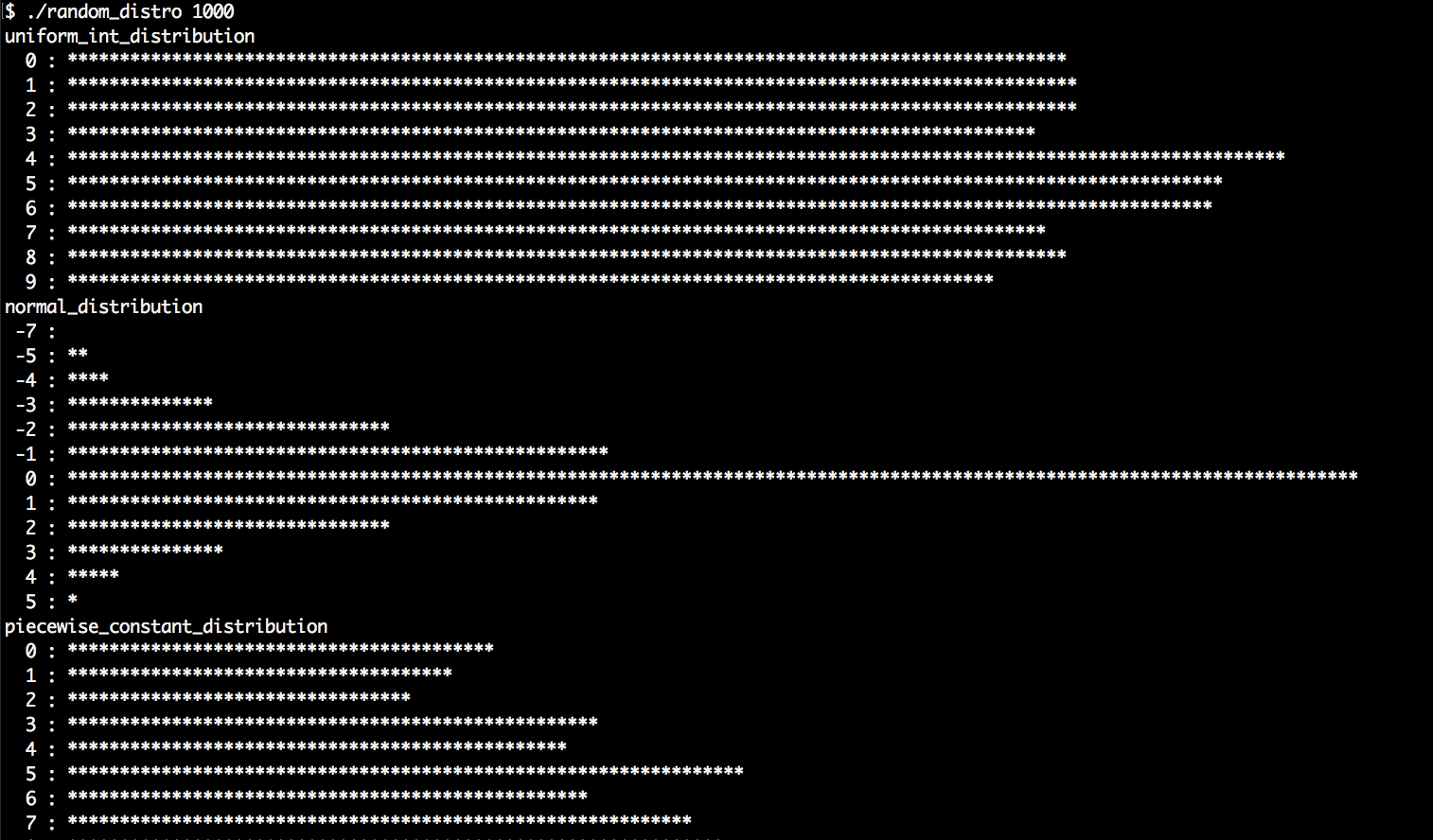
- Compiling and running the program yields the following output. Let's first run the program with 1000 samples per distribution:
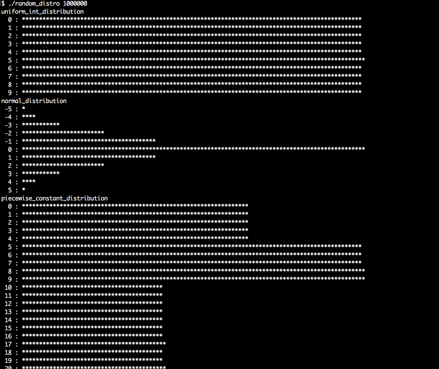
- Another run with 1,000,000 samples per distribution shows that the histograms appear much cleaner and more typical for each distribution. But we also see which ones are slow, and which ones are fast, while they are being generated: