The algorithm was invented in 1956 by Edsger W. Dijkstra, a computer scientist tasked to demonstrate the capabilities of the ARMAC computer while working at the Mathematical Center in Amsterdam.

Shortest path Dijkstra was the first algorithm implemented in pgRouting; pgRouting was called pgDijkstra in its early days.

The algorithm can be used by calling a pgr_dijkstra function. It has a few different signatures that let one calculate paths in the following modes:

• One-to-one: One source node to one target node
• One-to-many: One source node to many target nodes
• Many-to-one: Many source nodes to one target node
• Many-to-many: Many source nodes to many targets

All the methods can be used for either directed or non-directed networks.

The simplest usage of the algorithm looks like this:

select * from pgr_dijkstra('select gid as id, source, target, length_m as cost from pgr.ways', 79240, 9064); 

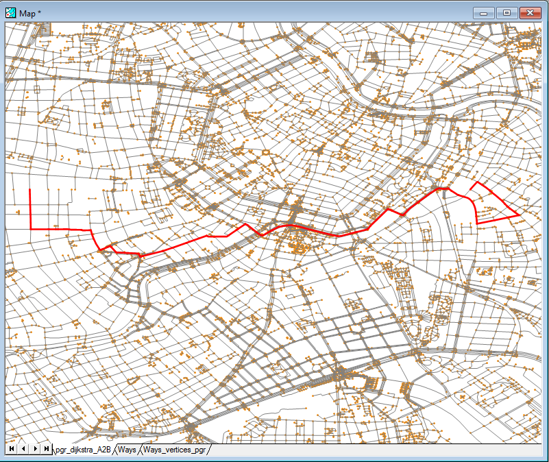
This uses the minimal signature of pgr_dijkstra and calculates the route from point A (in our case, Schottenfeldgasse) to point B (in our case, Beatrixgasse) and assumes a directed graph. The query results in 228 rows and the result looks as follows:

  seq|  path_seq|   node|   edge|             cost|         agg_cost 
-----+----------+-------+-------+-----------------+----------------- 
    1|         1|  79240|  69362| 169.494690094003|                0 
    2|         2|  52082|  44175| 107.754808368861| 169.494690094003 
... 

In order to obtain the actual geometry, we should modify the query a bit:

select  
   ways.the_geom 
from ( 
   select * from pgr_dijkstra('select gid as id, source, target, length_m as cost from pgr.ways', 79240, 9064)    ) as route 
   left outer join pgr.ways ways on ways.gid = route.edge; 

When visualized, our result looks as follows:

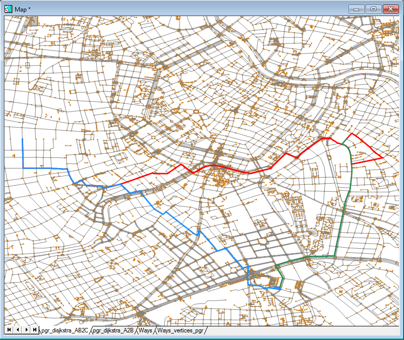
The output of the algorithm in the many mode is a bit different; the returned result set adds two extra columns (depending on the scenario) - start_vid and end_vid to specify the starting and/or the ending node, respectively. Let's use our previously used locations to search for the shortest path to Vienna's Central Train station:

select * from pgr_dijkstra('select gid as id, source, target, length_m as cost from pgr.ways', ARRAY[79240, 9064], 120829); 

The results are very similar, but you will notice the presence of a start_vid column, described earlier:

  seq|path_seq|start_vid|   node|   edge|       cost|       agg_cost 
-----+--------+---------+-------+-------+-----------+--------------- 
    1|       1|     9064|   9064| 209769|93.17915259|0 
    2|       2|     9064|  15615| 133330|82.53885472|93.179152510029 
... 

This time, our routes are as follows (the route between both points is also shown on the screenshot):

If you happen to only need the cost of the shortest path and you do not need the information about the vertices and edges per se, you can use the pgr_dijsktraCost function. It has the same signatures as the regular pgr_dijkstra, but returns simplified results:

select * from pgr_dijkstraCost('select gid as id, source, target, length_m as cost from pgr.ways', 79240, 9064); 
  start_vid|  end_vid|          agg_cost
-----------+---------+------------------
      79240|     9064|  5652.40083087719

And for a variation searching from two source nodes:

select * from pgr_dijkstraCost('select gid as id, source, target, length_m as cost from pgr.ways', ARRAY[79240, 9064], 120829); 
  start_vid|  end_vid|          agg_cost
-----------+---------+------------------
       9064|   120829|  2860.06209537015
      79240|   120829|  4532.12388804859