A final example of our pgRouting journey is a web application that consumes some of the functionality we have seen so far.

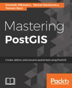
In order to preview the example, navigate to the example's folder - apps/pgrouting, run sencha app watch, and navigate to http://localhost:1841/apps/pgrouting/. You should see a similar output (you will have to calculate a route and drive time zone first though):

In order to feed our web app, we need to prepare a web service first. We have gone through creating a nice REST-like API for our WebGIS examples in the previous chapter, so this time all the maintenance stuff is going to be omitted.

At this stage, I assume our barebones web server is up and running, so we just need to plug in some functionality.

In order to perform any routing related logic, we should have the IDs of the vertices we would like to use in our analysis. Let's start with a function that snaps the clicked Lon/Lat to the nearest vertex in our network:

router.route('/snaptonetwork').get((req, res) => { 

    //init client with the appropriate conn details 
    let client = new pg.Client(dbCredentials); 

    client.connect((err) => { 
        if(err){ 
            sendErrorResponse(res, 'Error connecting to the database: ' + err.message); 
            return; 
        } 

        let query =  
`SELECT 
    id, lon, lat 
FROM 
    pgr.ways_vertices_pgr 
ORDER BY 
    ST_Distance( 
        ST_GeomFromText('POINT(' || $1 || ' ' || $2 ||' )',4326), 
        the_geom 
    ) 
LIMIT 1;`; 

        //once connected we can now interact with a db 
        client.query(query, [req.query.lon, req.query.lat], (err, result) =>{ 

            //close the connection when done 
            client.end(); 

            if(err){ 
                sendErrorResponse(res, 'Error snapping node: ' + err.message); 
                return; 
            } 

            res.statusCode = 200; 

            res.json({ 
                query: query, 
                node: result.rows[0] 
            }); 
        }); 
    }); 
}); 

The preceding method takes in a pair of coordinates expressing latitude and longitude and snaps them to the nearest vertex found in the network. It returns the ID of the node with its coordinates, as well as the query executed, so it is possible to see how our database is queried.

This API is used every time a map is clicked, in order to provide an input point for further processing.

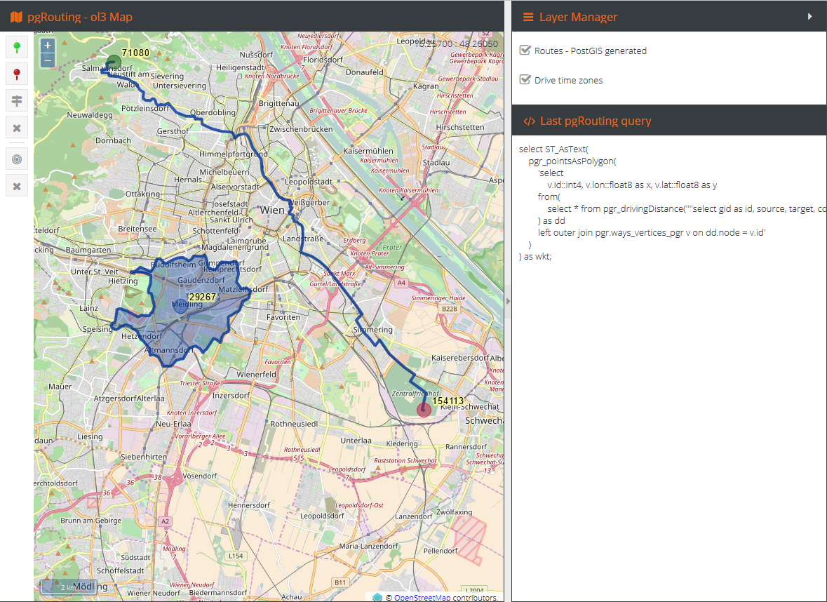
In the map client, one can use buttons with green and red pins to define start and end route points, respectively. Once this is done, a button with the map directions sign symbol triggers another API method call - the one that calculates the route. It takes in the IDs of nodes to calculate the shortest path between them:

let query =  
`select  
    ST_AsText( 
        ST_LineMerge( 
            ST_Union(ways.the_geom) 
        ) 
    ) as wkt 
from 
    ( 
        select 
            * 
        from 
            pgr_dijkstra( 
                'select gid as id, source, target, length_m as cost from pgr.ways', 
                $1::int4, $2::int4 
            ) 
    ) as route 
    left outer join pgr.ways ways on ways.gid = route.edge;`; 

We have seen a similar query already, when explaining how to get from a list of coordinates and edges output by the Dijkstra algorithm to the actual geometries representing the edges.

The preceding version does a few more operations - it unions the separate LineString edges into a MultiLineString geometry, then joins the MultiLineString into a single LineString to finally encode it as a WKT geometry, so our client app can handle it.

Because we use the minimal signature of the Dijkstra algorithm, it assumes the graph is directed, and this can be seen when our start point snaps to the edge of a dual carriage way and the general direction of a route is backwards:

We have a final method to implement in our pgRouting API - we need to calculate drive time zones. In this scenario, we take in a node ID and the driving time in seconds and output a polygon representing an alpha shape:

let query =  
`select ST_AsText( 
    pgr_pointsAsPolygon( 
        'select 
            v.id::int4, v.lon::float8 as x, v.lat::float8 as y 
        from( 
            select * from pgr_drivingDistance(''''select gid as id, source, target, cost_s as cost from pgr.ways'''', ' || $1 || ',' || $2 || ') 
        ) as dd 
        left outer join pgr.ways_vertices_pgr v on dd.node = v.id' 
    ) 
) as wkt;`; 

Once again, we have seen a similar query already; the difference is encoding the geometry as wkt.

The client side is rather simple and is pretty much about declaring the UI with some basic interactions, a map with the OSM base layer, and two vector layers with some customized styling. API calls use standard AJAX requests and then, on success, the executed query is displayed in the right-hand side panel and, also, the returned WKT is parsed and displayed on the map. Nothing fancy really.

It is worth noticing though, that the map projection in this example is EPSG:3857 and the network data is in EPSG:4326. So the geometries need to be re-projected before being sent out to the API and, when the WKT geometry is retrieved, it needs to be displayed on a map.

The full source code of this example can be found in this chapter's resources, so you may study it in detail as needed.